UCGE Reports
Number 20253
Department of Geomatics Engineering
X86-Based Real Time L1 GPS Software Receiver
(URL: http://www.geomatics.ucalgary.ca/research/publications/GradTheses.html)
by
Shahin Charkhandeh
Date
April 2007
iii
Abstract
Given the demanding computational requirements of software-based GPS receivers, high
data processing efficiency is required to obtain real-time performance. There are two
basic approaches to accomplish this: reducing the number of computations required, or
improving the efficiency with which the computations are carried out. This work takes
the latter approach, primarily by using the MMX technology available on x86-compatible
processors to more rapidly perform the Doppler removal and code correlation
computations. Other computational saving methods are also described. Using this
approach, computational improvements of greater than 70% are realized over the
standard (integer math) implementation. Test results indicate that tracking performance
of the software receiver is reasonable and that position and velocity accuracies are at the
metre and decimetre per second level, respectively. Chapter one covers an introduction
into GPS receiver architecture, software receivers and the needs for them. Chapter two
describes in detail the theoretical aspects of different components and algorithms used in
the receiver. Chapter three covers the real time operation of the GPS software receiver. It
looks into the challenges and issues which needed to be addressed to achieve the real
time operation in the receiver. Chapter four presents results of static and dynamic tests
iv
Acknowledgement
Dr. Gérard Lachapelle:
There is no word that can describe my indebtedness to you. Your kindness and support
has been exemplary and more than I could ever imagine. You are my mentor, my role
model and a man whom I strive to be in my professional life. You have impacted my life
in many ways and I am a better person because of being your student for two years.
Thank you for everything.
Dr. Mark Petovello
This work would have not been possible without your help. You were there every time
that I needed help and faced a road block. I am in debt to you for ever.
Mom and Dad
You are the pure symbols of honesty, love and sacrifice. You are the stars of my life and I
am proud to be your son. I dedicate this work to you as small token to show you my
v Table of Contents Approval Page... ii Abstract ... iii Acknowledgement ... iv Table of Contents ...v
List of Tables ... vii
List of Figures ... viii
Notation... x
Abbreviation and Acronyms ...x
CHAPTER 1 ...1
INTRODUCTION ...1
1.1 FPGA-Based Vs PC-Based software receiver ...3
CHAPTER 2 ...9
2.1 GPS Signal Structure ...9
2.1.1 GPS Carrier...9
2.1.2 Coarse-Acquisition (C/A) and Precise (P) codes...9
2.1.3 Generation of C/A code ...11
2.1.4 Navigation data bits ...15
2.2 GPS Receiver Architecture ...17
2.2.1 RF Front-End ...17
2.2.2 GPS C/A Code Acquisition ...23
2.2.3 GPS Signal Tracking...31
2.2.4 Pseudo-range derivation...38
CHAPTER 3 ...45
REAL-TIME GPS RECEIVER DESIGN ...45
3.1 Computational Bottlenecks...45
3.2 Doppler Removal ...48
3.2.1 Generation of sine and cosine values...48
3.2.2 MMX Technology ...52
3.2.3 Code Correlation using SIMD ...54
3.2.4 Software Architecture ...56
CHAPTER 4 ...63
TEST SET RESULTS...63
vi 4.2 Real-time Performance ...71 4.3 Acquisition Performance ...74 4.4 Tracking Performance...77 4.5 Position Accuracy ...81 CHAPTER 5 ...90
CONCLUSIONS AND RECOMMENDATIONS ...90
5.1 Front-end and Acquisition component ...91
vii
List of Tables
Table 1: Characteristics of GPS codes... 10
Table 2: Combination of phase selection for C/A code... 12
Table 3: Common Costas Loop discriminator used in GPS receivers (Ward 1996) ... 34
Table 4: Common GPS receiver FLL discriminators (Ward 1996)... 35
Table 5 : Common Delay lock loop discriminators (Ward 1996) ... 36
Table 6: Loop filter characteristics (Ward 1996)... 38
Table 7: Computational load of the receiver to track six satellites... 46
Table 8: Computational load of the receiver for tracking 6, 8 and 12 satellites ... 46
Table 9: Performance Comparison ... 72
Table 10: Acquisition Speed ... 74
Table 11: Position error statistic ... 82
Table 12: Position error difference with OEM4 ... 84
Table 13: Position error statistics... 87
viii
List of Figures
Figure 1: Block diagram of C/A code generation ... 11
Figure 2 : Autocorrelation of Satellite 1 ... 14
Figure 3 : Cross correlation of Satellite 1 and 15 ... 14
Figure 4 : TLM and HOW words ... 16
Figure 5: Block diagram of GPS Front-End ... 17
Figure 6 : Mixing operation ... 18
Figure 7 : Conversion to base-band (analog mixing)... 20
Figure 8: Intermediate frequency sampling process ... 23
Figure 9 : Block diagram of signal acquisition ... 24
Figure 10: Probability density function for different SNR ... 26
Figure 11: Tong search detector algorithm ... 28
Figure 12: Code and carrier tracking loops... 32
Figure 13: Code mismatch early, prompt and late components... 37
Figure 14: Diagram of a result of Bit synchronization ... 39
Figure 15: Pseudorange derivation ... 44
Figure 16: SIMD instruction versus SISD ... 53
Figure 17: Over all Architecture of the software ... 59
Figure 18: Acquisition flow chart ... 61
Figure 19: Doppler removal, Correlation and tracking flow chart ... 62
Figure 20: Frontend and test set up... 65
Figure 21 : 6-tap band-pass filter ... 67
ix
Figure 23: 20-tap band pass filter ... 68
Figure 24: PSD of incoming signal using a 20-tap filter ... 68
Figure 25: Digital down conversion in FPGA ... 69
Figure 26: Data Collection set up for Performance Testing ... 71
Figure 27: 1 ms coherent integration ... 74
Figure 28: 2 ms Coherent Integration ... 75
Figure 29: Estimated C/N0 for all PRNs ... 77
Figure 30: Doppler value for PRN 23... 79
Figure 31: Doppler value for PRN 22... 80
Figure 32: PLL Lock detector output... 81
Figure 33: Scatter plot of North and East errors ... 82
Figure 34: Solution error difference with OEM4 ... 83
Figure 35: Pseudorange errors ... 84
Figure 36: Software receiver-Derived velocity errors ... 85
Figure 37: Scatter plot of North and East error... 86
Figure 38: Position error versus time... 86
Figure 39: Velocity error versus time ... 88
x
Notation
Abbreviation and Acronyms
ABAS Airborne – Based Augmentation System
ADC Analog to Digital Converter
ASIC Application Specific Integrated Circuit
ANSI American National Standard Institute
AD Analog to Digital Converter
BPSK Bi-Phase Shift Keying
BOC Binary Offset Carrier
CA-Code Coarse Acquisition Code
C/N0 Carrier to Noise Ratio
CPU Central Processing Unit
DFT Discrete Fourier Transform
DLL Delay Lock Loop
DMA Dynamic Memory Access
DoD U.S. Department of Defence
DOP Dilution of Precision
DoT Department of Transportation
EGNOS European Navigational Geostationary Overlay Service
EU European Union
ESA European Space Agency
xi FLL Frequency Lock Loop
FPGA Filed Programming Gate Array
GBAS Ground-Based Augmentation Systems
GPS Global Positioning Systems
GNSS Global Navigation Satellite Services
HOW Hand Over Word
IF Intermediate Frequency
IPEXSR Institute of Geodesy and Navigation PC-based Experimental Software Receiver
LAAS Local Area Augmentation System
LO Local Oscillator
MLS Maximum-Length Sequence
MM0 - MM7 MMX registers
NI National Instrument
NCO Numerically Control Oscillator
PLAN Position, Location And Navigation
PC Personal Computer
P-Code Precise Code
PLL Phase Lock Loop
PRN Pseudo Random Noise
PSR Purdue Software Receiver
Q Quality factor of band pass or notch filter
xii RF Radio Frequency
RMS Root Mean Square
SBAS Satellite - Based Augmentation Systems
SIMD Single Instruction Multiple Data
SISD Single Instruction Single Data
SSE Streaming SIMD Extension
0 N
S Signal to Noise Ratio
TLM TELEMETRY
TRIGR Transform-Domain Instrumentation Global Positioning System
(GPS) Receiver
UHF Ultra High Frequency
UTC Universal Time Coordinated
Chapter 1
Introduction
The evolution of technology has increased the demand for higher accuracy, availability
and reliability in positioning services. The new requirements increased the need for
modernization of current GNSS and also developing new systems that will complement
GPS I. Satellite Based Augmentation Systems (SBAS), Ground Based Augmentation
Systems (GBAS), Airborne Based Augmentation System (ABAS), US Wide Area
Augmentation System (WAAS), Local Area Augmentation System (LAAS) and
European Navigational Geostationary Overlay Services (ENGOS) are some of the
popular systems that complement GPS to improve performance. However, all the above
systems’ performances are still limited due to original design of GPS.
Consequently, the experiences gained in the design of GPS and high market demands
have initiated a desire for new signals and constellations. The US Department of Defence
(DoD) and Department of Transportation (DoT) have started a GPS modernization
process, called GPS II and GPS III. The European Union (EU) and the European Space
Agency (ESA) decided to launch their own GNSS constellation known as Galileo. Also,
the Russian space program has decided to enhance its GLONASS.
Modern GPS receivers usually use Application Specific Integrated Circuit (ASIC) for
advantage of using an ASIC for signal processing is high speed and low power
consumption. ASIC chips can not be recompiled like general purpose processors,
therefore they are expensive to redesign and modify.
This highlights the main advantage of software receivers. It allows the user to redesign
the system and to test new algorithms. It is fairly inexpensive and easy to modify a
software receiver that is running on a programmable microprocessor. Also, as mentioned
above, the arrival of new signals requires new algorithms to be developed and tested.
Software receivers allow the developer to work on these algorithms and have more
control on them.
Research on GPS software started about ten years ago but because of limitations in the
computational power that was available at that time, the initial systems have been slow
and inefficient. However, as computational power has increased, there has been renewed
attention in this field. A lot of research has been done on different optimization
techniques to make the receiver as fast as possible and eventually reach real time
performance.
This work focuses on the difficulties that exist which limit the real time operation of a
GPS receiver and how to over come them. Chapter 2 of this thesis covers the fundamental
theory related to GPS receivers. Specifically, it covers concepts from the front-end,
acquisition, tracking and solution calculations. Chapter 3 discuses the optimization
techniques used in the software receiver developed herein. Chapter 4 demonstrates the
results achieved and finally, in chapter 5, conclusions are presented along with a
There are typically two kinds of software receivers, PC-based and FPGA based. In this
section, we briefly describe the work which has been done in each of these areas and the
comparisons between the two approaches.
1.1 FPGA-Based Vs PC-Based software receiver
There are typically two different approaches toward software receiver design. The first
approach is a complete PC based “software receiver” which processes the digitized
intermediate frequency within the CPU of the personal computer. All the signal
processing is done inside the PC processor.
In the other approach, the complete base-band processing is performed within the field
programmable gate array (FPGA) thus reducing the load on the PC processor. In this
method, all the high speed signal processing tasks are completed in FPGA while the
lower rate tasks such as navigation calculations are performed in the PC. Both approaches
offer a good degree of control over the base-band processing and the capability of testing
algorithms side by side.
One of the major requirements for this work was to develop software that can be used as
a research tool. Therefore, the PC-Based approach was chosen since it will allow
researchers that may not be familiar with FPGA to run and use the tool on their PCs.
Selected previous work in this field is summarized below.
IPEXSR (Institute of Geodesy and Navigation PC-based Experimental Software
Receiver) is a PC based software GNSS receiver that is developed in University FAF
program. Real signals are digitalized by an NI 5112 analog to digital conversion (ADC)
card which is connected to a low bandwidth (2.5 MHz) GP 2010 L1 front-end. This
receiver has the capability to work in real time mode (connected to the front-end) and
high speed off line (reading from the data file). It uses FFT/DFT techniques to perform
code phase and Doppler search. FFT/DFT techniques for acquisition will be described in
detail in next chapter of this thesis. The Tracking component of the receiver works in two
modes, normal and under sampling.
In under sampling mode, only every x’th sample is processed. The main purpose of this
method is to reduce the processing demands by a factor of x as discussed in the paper.
Under sampling decreases the signal to noise ratio by 10 log(x), but does not have any
other effect on the tracking performance, even though the Nyquist criterion may not be
fulfilled. In Normal Mode of operation, the tracking module makes use of highly
optimized code using the SSE2/3 instruction sets. The receiver can track nine channels in
real-time with a sampling rate of 4.096 MHz on a single Pentium IV running at 3 GHz.
The receiver was able to achieve a positioning accuracy of -0.5 m in longitude, -0.7 m in
latitude error and -1.5 m in height.
GPSrxis another real-time GPS software receiver which has been developed in Stanford
University (Akos et al 2001). The entire receiver algorithms are written using ANSI C.
The receiver provides sub-second acquisition and solves for the position in real-time
using four channels on a 650 MHZ x86 compatible processor. The front-end is a single
stage frequency down conversion with band pass sampling. The IF 3 dB bandwidth is 2
MHz and the sampling frequency can be in the range of 4-6 MHz. There was a direct
from using the MMX/SSE instruction sets. All the algorithms are highly optimized C
routines. An FFT-based circular convolution technique is used for acquisition. The PRN
code tracking is done using a traditional non-coherent second order delay lock loop
(DLL). Tracking the carrier is solved using a dynamic combination of frequency and
phase lock loops (FLL/PLL). The result presented showed a position solution with errors
significantly less than 100 m. One of the reasons for the higher error magnitude,
although acceptable, is the limitation due to the narrow bandwidth front end design.
A Real time GPS civilian L1 software receiver was also developed by Cornell University
(Ledvina et al 2003). The receiver consists of an RF front end, a system of shift registers
and DAQ card and a PC running an Intel Pentium 4 at 1.7 GHz. The RF front-end down
converts the signal into a 2-bit digital data stream at 5.714 MHz. The Base band mixing
of the local code and incoming data is accomplished through a bit-wise parallel operation.
Bit-wise parallel operations work with representations of data that store successive
samples in successive bits of a word. For example, 32 samples of the RF front-end output
are stored in two 32-bit words. One word stores the 32 sign bits of the 32 samples, and
the other word stores the 32 magnitude bits. The stored tables of the base-band mixing
cosine and sine waves have their sign and magnitude bits stored in separate words, with
each 32-bit word storing 32 sign or magnitude bits that tabulate to 32 successive samples
of the corresponding cosine or sine waves. Similarly, the stored tables of the prompt and
early-minus-late codes store sign or sign and zero-mask bits in words with each word
storing 32 samples worth of data. With this scheme, the EXCLUSIVE OR operations that
EXCLUSIVE OR command and other bit-wise commands that operate in parallel on each
of two input arguments' 32-bit pairs (Ledvina et al 2003). The receiver is able to run 10
channels in parallel and in real time while providing 10-15 m position navigation
accuracy for standalone applications (roof top antenna).
The receiver was later modified to process Galileo signals (Ledvina et al 2006). The work
showed the interoperability between a GPS and Galileo real-time software receiver. The
real-time capability of this receiver is based mainly on two technologies.
The first technology, called bit-wise parallel signal processing (described above) allows
the receiver to process 32-64 RF samples in parallel. The second technology is a method
for efficient real-time generation of over-sampled bit-packed PRN codes. This
technology is helpful since Galileo L1 signal have longer periods than the L1 C/A code
signals (Ledvina et al 2006). It is usually a common approach in a software receiver
design to store replica PRN codes to reduce the computational real-time needs. However,
the longer length of Galileo L1-B and L1-C BOC (1, 1) PRN codes makes this method
less attractive due to the additional memory requirements for storing the longer codes.
This can be a problem especially in embedded platforms. This second technology
addressed this issue while adding some computational cost to the receiver design
(Ledvina et al 2006).
The Purdue Software Receiver (PSR) is a real-time software receiver developed at
Purdue University for research and teaching purposes (Heckler & Garrison 2004).
in modern x86 and Power PC processors. The Software is coded in C++ making use of
threaded objects to encapsulate functions and related data together, and to reduce
unnecessary copying of data (Heckler & Garrison 2004).
The PSR utilizes the 16 bit signed integer data type as its basic data element. Sixteen
signed bits of precision guarantees enough dynamic range to prevent overflow during the
multiplication stage of the correlation algorithm using the common 1 to 2 bit quantized
GPS signal, 1 bit raw PRN code, and several bits for a digital sinusoid. In addition, the 16
bit signed integer corresponds to the word type associated with x86 SIMD operations.
Using the original 64-bit MMX registers, four samples are operated upon in parallel.
With the expanded 128 bit SSE registers found in more recent CPUs, eight samples can
be processed with a single operation. Real time operation of the receiver was
demonstrated by forcing the receiver to process 100 seconds of data. In order to remove
latency involved with disk access, the 100 seconds of raw GPS data was buffered
completely into RAM (not reading from a file) before processing. The raw GPS data was
sampled at 2.3333 MHz, leading to a correlation length of 2333 samples. The receiver
was able to process this data in less than 100 seconds while running 12 channels.
However, there was no information in the paper about the accuracy of the navigation
solution computed by the receiver.
A Transform-Domain Instrumentation Global Positioning System (GPS) Receiver
(TRIGR) was developed at Ohio University (Soloviev et al 2005). The concept behind
and have it reveal ‘everything’ that one needs to know about the GPS signal. This
instrument does not operate in real-time but uses a GPS software receiver at its heart.
Signal processing of the TRIGR is a combination of batch and sequential processing
techniques. The receiver uses a FFT approach in the acquisition component. CA code
and carrier tracking measurements are applied to aid the sequential correlators for the
tracking of the P code GPS signal. CA-code measurements set up parameters of the
replica carrier and replica P-code to wipe-off the carrier and P-code signal components
from the incoming L1 or L2 encrypted P(Y) code signals.
The work presented in this thesis attempts to combine different techniques presented in
some of the above work to design, develop and test a real-time GPS software receiver.
The focus of the work was on real-time operation of the receiver and employing
algorithms that can help one achieve that level of performance. As discussed later, there
are some trades off in using some of these algorithms (small hit on the accuracy of the
receiver). This work is unique in the sense that it takes the use of SIMD instructions to
the next level and shows how useful this features can be in GPS software receiver design.
As has been presented earlier, software receivers are the heart of many different
applications such as TRIGER (Soloviev et al 2005). The work contained in this thesis can
Chapter 2
GPS Receiver Theory
This chapter describes the properties of the GPS signal and operations performed inside
the GPS receiver to process this data and compute a navigation solution.
2.1 GPS Signal Structure
2.1.1 GPS Carrier
GPS signals are transmitted on one of two radio frequencies in the UHF band (Tsui &
James 2000). The two frequencies (L1 and L2) are derived from the fundamental
frequency f0 = 10.23 MHz :
fL1= 1575.42 MHz = 154 f0 (2.1) fL2=1227.6 MHz = 120 f0 (2.2)
The wavelengths of the carriers are:
λL1 = 19.03 cm (2.3)
λL2 = 24.42 cm (2.4)
2.1.2 Coarse-Acquisition (C/A) and Precise (P) codes
GPS Pseudo-Random Noise (PRN) code is a binary sequence that appears to be random
Table 1: Characteristics of GPS codes
Parameter C/A-Code P-Code
Chipping Rate (chips/s) 1.023 e6 10.23 e6
Chipping Period (ns) 977.5 97.75
Range of One Chip (m) 293.0 29.30
Period of the Code 1msec 1week
The GPS signal is a phase-modulated signal with an initial phase of zero or π ; this type of phase modulation is referred to as bi-phase shift keying (BPSK). The spectrum shape
can be described by the sinc function (sinx/x) with a spectrum width proportional to the
chip rate. As an example, if the chip rate is 1 MHz, the main lobe of the spectrum has a
null-to-null width of 2 MHz.
The P-code, when encrypted, is termed Y-code. Y-code is classified and unauthorized
users cannot access it. (Tsui & James 2000).
2.1.3 Generation of C/A code
The GPS signal is from a family of pseudorandom noise (PRN) codes known as Gold
codes (Tsui & James 2000). Signals are created as the product of two 1023-bit PRN
sequences G1 and G2. A maximum-length linear shift 10 stage register driven by a 1.023
MHz clock generates the G1 and G2 signals. A maximum-length sequence (MLS)
generator can be formed from shift registers with proper feedback. The feedback of G1 is
from bits 3 and 10 as shown in figure one and corresponds to the polynomial G1: 1 +
X3+X10. The feedback of G2 is from bits 2, 3, 6, 8, 9 & 10 as shown in figure 1.
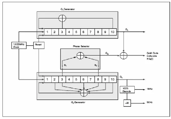
Figure 1: Block diagram of C/A code generation
The corresponding polynomial is G2: 1+X2+X3+X6+X8+X9+X10. To make different C/A codes for satellites, the outputs of the two shift registers are combined in a special
manner. G1 always supplies its output, but G2 supplies two of its states to a modulo-2
adder to generate its output. The selection of states for the modulo-2 adder is called phase
selection. Table 2 shows the combination of phase selections for each C/A code. It also
shows the first 10 chips of each code in octal representation. Note that only the first 32 of
the 37 possible codes are used as Satellite C/A codes. The remaining five codes are
reserved for other uses e.g. ground transmitters (pseudolites).
Table 2: Combination of phase selection for C/A code Satellite ID Number GPS PRN Signal Number Code Phase Selection Code Delay Chips First 10 Chips C/A Octal 1 1 2⊕6 5 1440 2 2 3⊕7 6 1620 3 3 4⊕8 7 1710 4 4 5⊕9 8 1744 5 5 2⊕10 17 1133 6 6 1⊕8 18 1455 7 7 2⊕9 139 1131 8 8 3⊕10 140 1454 9 9 2⊕3 141 1626 10 10 3⊕4 251 1504 11 11 5⊕6 252 1642 12 12 6⊕7 254 1650 13 13 7⊕8 255 1764 14 14 8⊕9 256 1772 15 15 9⊕6 257 1775 16 16 2⊕10 258 1776 17 17 1⊕4 469 1156 18 18 2⊕5 470 1467
19 19 3⊕6 471 1633 20 20 4⊕7 472 1715 21 21 5⊕8 473 1746 22 22 6⊕9 474 1763 23 23 1⊕3 509 1063 24 24 4⊕6 512 1706 25 25 5⊕7 513 1743 26 26 6⊕8 514 1761 27 27 7⊕9 515 1770 28 28 8⊕10 516 1774 29 29 1⊕6 859 1127 30 30 2⊕7 860 1453 31 31 3⊕8 861 1625 32 32 4⊕9 862 1712 ** 33 5⊕10 863 1745 ** 34* 4⊕10 950 1713 ** 35 1⊕7 947 1134
2.1.3.1 C/A code correlation properties
C/A codes have high autocorrelation peaks and low cross-correlation peaks. Different
C/A codes have a cross correlation of -65/1023 (occurrence 12.5 %), -1/1023 (75%) and
63/1023 (12.5%) (Tsui & James 2000). Figure 2 and Figure 3 show the autocorrelation
Figure 2 : Autocorrelation of Satellite 1
The above figures show that the maximum autocorrelation peak is 1023, equal to the C/A
code length. The other correlation values are 63,-1 and -65 as mentioned above.
2.1.4 Navigation data bits
The C/A code is a bi-phase coded signal, which changes the carrier phase between Zero
and π at a rate of 1.023 MHz (Tsui & James 2000). The navigation data bit is a bi-phase
code as well at a rate of only 50 Hz, which translates to each data bit being 20 ms long.
Since the C/A code is 1 ms, there are 20 C/A codes in one data bit. Therefore, in one data
bit all 20 C/A codes have the same phase. A phase transition due to the data bit causes a
phases difference of ±πin two adjacent C/A codes.
The navigation data message is divided into a 1500-bit long frame containing 5
sub-frames, each 300 bits long. Each sub-frame contains ten words, each word being 30 bits
long. Sub-frames 1, 2, and 3 are repeated in each frame. Sub-frames 4 and 5 have 25
different versions referred to as pages 1 to 25. Considering a bit rate of 50 bps, the
transmission of a sub-frame lasts 6 seconds, a frame lasts 30 seconds and an entire
navigation message lasts 12.5 minutes (ICD-GPS-200 2003).
2.1.4.1 TELEMETRY (TLM) and HAND OVER WORD (HOW)
The first two words of all the sub frames are the telemetry (TLM) word and hand over
word (HOW) (Tsui & James 2000). Each has a length of 30 bits. Figure 4 shows the
structure of these words. The TLM word starts with an 8-bit preamble, followed by 16
Figure 4 : TLM and HOW words
In addition to the TLM and HOW words, there are eight other words in each sub frame.
Below is a brief description of data in these words. For a complete description, one can
refer to the ICD-GPS-200 document. Sub-frame 1 contains some clock information. That
is information necessary to calculate the time of transmission for the navigation message
from the satellite. In addition, sub-frame 1 contains health data indicating whether the
data is corrupted. Sub-frames 2 and 3 contain the satellite ephemeris data. The ephemeris
data provides the satellite orbits, needed to calculate accurate satellite positions.
As mentioned earlier, the last two frames repeat every 12.5 minutes giving 50
sub-frames. Sub-frame 4 and 5 contain almanac data. The almanac data is the ephemeris and
clock data with reduced precision. Additionally, each satellite transmits almanac data for
sub-frames 4 and 5 contain various data such UTC time parameters, health indicators, and
ionosphere parameters.
2.2 GPS Receiver Architecture
2.2.1 RF Front-End
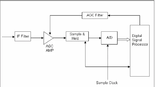
Figure 5: Block diagram of GPS Front-End
The first component after the antenna is usually an amplifier or filter.
The noise figure of a receiver is (Tsui & James 2000):
N N G G G F G G F G F F F ... 1 ... 1 1 2 1 2 1 3 1 2 1 − + + − + − + = (2.5)
where Fi and Gi (i = 1, 2 . . . N) are the noise figure and gain, in linear terms, of each
individual component in the RF chain. If the amplifier is the first component, the noise
figure of the receiver is low and is approximately equal to the noise figure of the first
Therefore, the noise contribution caused by the second component e.g. a filter, is reduced
by the gain of the preceding amplifier. However, strong signals within the bandwidth of
the amplifier may drive it into saturation and generate spurious frequencies.
On the other hand, if the first component is a filter it can stop out-of-band signals from
entering the input of the amplifier. A filter with 2 MHz bandwidth (to pass only C/A
code) with a center frequency at 1575.42 MHz is considered high Q (Quality Factor)
Usually, the insertion loss of such a filter is relatively high, about 2 to 3 dB, and the filter
is bulky. The receiver noise figure with the filter as the first component is about 2–3 dB
higher than in the previous arrangement (Tsui & James 2000).
2.2.1.1 Mixing Operation and Intermediate Frequency Filtering
Down conversion from RF to IF is accomplished by mixing the incoming signal and
noise with a local oscillator signal (LO). This process is illustrated in figure 6.
A GPS signal may be represented by:
[
( 0 ) 0]
cos ) ( ) ( ) (t = AC t D t ω +∆ω +Φ s (2.6) where A = signal amplitude C(t) = PRN code modulation D(t) = 50bps data modulation = = 0 0 2πf ω Carrier frequency (L1 or L2) = ∆ =∆
ω
2π
f Frequency offset (Doppler, etc)=
Φ0 Nominal but ambiguous carrier phase.
Therefore, the result of the mixing (ignoring the harmonics, LO feed through and image
noise) of GPS signal and LO signal (LO1(t)=2cosω1t ) is:
[
]
[
]
{
cos( 0 1 ) 0 cos( 0 1 ) 0}
) ( ) ( ) (t = AC t D t + +∆ t+Φ + − +∆ t+Φ sIF ω ω ω ω ω ω (2.7)The upper side band is not of any interest and can be eliminated via a low-pass filter. This
will result in an IF frequency ofωIF =ω0−ω1.
2.2.1.2 Conversion to Baseband
Conversion to baseband means synthesizing the IF signal to that of in-phase and
quadra-phase components of the signal envelope. This can be accomplished by analog
Analog mixing, illustrated in figure 7, is realized by mixing the IF signal with two local
carriers, one of which is phase shifted by 90◦ with respect to the other (in quadrature).
The resulting in-phase and quadra-phase signals are as follow:
t t LO2I( )= 2cos
ω
2 (2.8) ) sin( 2 ) 2 cos( 2 2 2 2 t t LO Q =ω
+π
=−ω
(2.9) ) cos( ) ( ) ( 2 ) (t = A C t D t ∆ t+Φ0 Is ωB (2.10) ) sin( ) ( ) ( 2 ) (t = A C t D t ∆ t +Φ0 Qs ωB (2.11)where the residual frequency offset is:
ω
ω
ω
ω
= − +∆∆ B IF 2 (2.12)
Figure 7 : Conversion to base-band (analog mixing)
Intermediate sampling (IF sampling) shown in Figure 8 (Van Dierendonck 1996) is based
on the concept of sampling the IF signal at rate which the Q samples and I are obtained
directly.
N f
SR= 4 IF (2.13)
where
f
IF is the IF frequency being sampled and N is an odd number. Therefore, thesignal will be sampled at intervals tk where:
,... 1 , 0 sec; 4 = = k f kN t IF k (2.14)
Sampling the signal at this rate will result in the following:
Φ + = Φ + ∆ + = Φ + ∆ + = = k k k IF k k IF IF k k k IF k kN D AC f f kN D AC f kN f f t D t AC t s s 2 cos ) 1 ( 2 cos 4 ) ( 2 cos ) ( ) ( ) ( 0 0 π π π (2.15)
where the ∆f is the offset due to Doppler, Ckand Dkare the code and data at timetk, and
k k IF k t f f kN ∆Φ + Φ = ∆ + Φ = ∆ + Φ = Φ 0 0 0 2 ω π (2.16)
is the baseband phase of the sample attributable to the nominal phase and frequency
offset at time
t
k . It can be noted from equation 2.15 (ignoring∆f ) that IF signalssampled at exactly 90◦ phase result in the following sequence of samples based on values
of N:
[
, , , , , ,...]
2 Isk Qsk −Isk −Qsk Isk Qsk or[
, , , , , ,...]
2 Isk −Qsk −Isk Qsk Isk −QskIt is interesting to notice the negative samples and the meaning of it. To explain this
further, one need to drive the formulas as follow:
k I N k s N N k N k s N k Q N k k k N k s k I k s − = Φ + − = + = + Φ + = Φ + + = + Φ + = = + Φ + = Φ + + = + = ) 0 2 cos( 2 ) 2 2 0 2 cos( ) 0 ) 2 ( 2 cos( 2 ) 0 2 sin( )) 2 ( 0 2 cos( ) 0 ) 1 ( 2 cos( 1 π π π π π π π π
This method is also called pseudo sampling, since the I and Q samples do not occur at
the same time. There could be potential problems with this method however. If dealing
with large frequency offsets with respect to the sampling frequency, this method can
create an extra phase shift in the quadra-phase samples, causing aliasing to a negative
frequency offset. However, this is not a problem for a GPS signal with reasonable
Doppler.
One of the advantages of this method is that, because Q and I samples are generated in
the same circuitry there are no gain or phase imbalances between them as compared to
the analog base-band conversion process. In addition, there is only one A/D converter
needed in this method. However, there are certain disadvantages that come with using
this approach. One is that the aperture time of sampling process must be small with
respect to the period of the IF frequency.Given, Sin(x)/x, where x is proportional to the
product of the frequency and the aperture time, attenuation occurs if the aperture time is
Figure 8: Intermediate frequency sampling process
2.2.2 GPS C/A Code Acquisition
The first step in the operation of GPS receiver is to find a rough estimate of the PRN code
offset and carrier Doppler. Acquisition is a coarse synchronization process which
determines the estimate of PRN code and Doppler. This information is used to initialize
tracking loops for signal tracking and navigation data demodulation. GPS signal
acquisition is essentially a two-dimensional search process in which a replica code and a
replica carrier are aligned with the received signal.
The correct alignment is identified by measurement of the output power of the
correlators. When both the code and the carrier Doppler match the incoming signal, the
two-dimensional search consist of an estimate of the code offset to within half a chip and
a Doppler estimate to within the lock range of the tracking loops. This process is shown
in figure 9.
Figure 9 : Block diagram of signal acquisition
The two-dimensional search space covering the full range of the ambiguity of code and
Doppler needs to be defined before acquisition can be performed. The Doppler search
space can be reduced if the initial estimate of the Doppler is available. If such an estimate
is not available, a search space of -5 kHz to +5 kHz is appropriate for GPS signals. The
frequency bin size is calculated as follow (Van Dierendonck 1996):
T f 3 2 = ∆ (2.17)
where
∆
f
is the size of a frequency bin, in Hz, and T is the coherent integration time (or dwell time) in seconds. As this formula illustrates, there is a trade off between thebetter frequency resolution and higher sensitivity, however it increases the number of
frequency bins that needs to be searched. The code search space usually includes all
possible code offsets. The resolution of the code search needs to be smaller than half a
chip. The sampling frequency is usually used to specify this resolution.
2.2.2.1 Detection Criteria
As was briefly mentioned earlier, acquisition is based on the measurement of correlator
output (Krumvieda et al 2002). The correlators provide a measure of the total I and Q
signal value over the coherent integration time (dwell time).
The envelope of the acquisition result I2 +Q2 is a measure of the amplitude of the signal. When the local code and incoming signals are aligned, the amplitude of the
recovered signal is at a maximum. The In-phase and Quadra-phase components I and Q
are calculated by stripping off the reference code and the carrier from the received signal
as shown in figure 10. The envelope is then computed and compared with a threshold.
Since the GPS signal is buried in noise, a threshold must correspond to an acceptable
probability of false alarm. A false alarm is the probability of detecting a signal from a
The threshold can be set as follow:
fa n
t P
V =σ −2ln (2.18)
where Pfais the single trial probability of false alarm, and σn is the 1-sigma noise
amplitude. σnis frequently obtained by using a reference PRN which is known to be
absent such as PRN 37.
Any cell amplitude that is at or above the threshold is considered to have a signal present.
The detection of the signal is a statistical process because each cell contains either noise
with the signal present or noise with the signal absent (Krumvieda et al 2002).
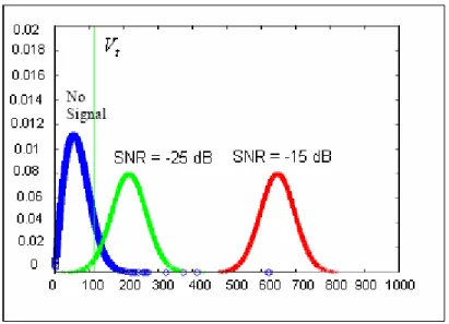
Figure 10: Probability density function for different SNR
Figure 10 illustrates that if the SNR is high, it is easy to set a threshold that provides both
low probability of a false alarm and low risk for missed detection. However, for a lower
Looking at Figure 10, the possibility of missed detection is the area under the green curve
from the threshold line to left. This is the probability that there is a signal but the
threshold is set too high. Probability of false detection is the area under the blue curve
from the threshold line to the right. This indicates that there is no signal but since the
threshold was set too low, we mistakenly declared the signal present. There is a trade off
when setting the threshold to avoid false alarms. If the threshold is set very high to avoid
falsedetections, then there is a high probability that weak signals will not be detected. In
GPS this is the typical situation and single trial detection is not effective. It is important
to note that when a signal is absent, the envelope has a Rayleigh distribution. Otherwise
the envelope has a Ricean distribution (I and Q signals are normally distributed if the
noise is Gaussian).
There are several different search methods for the acquisition of GPS signals presented in
the literature. Two common approaches are described here.
Tong detector method:
The Tong detector has a reasonable computational burden and is excellent for detecting
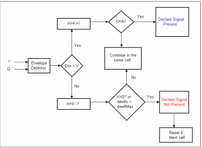
signals with an expected C/No of 25 dB-Hz or higher. Figure 11 presents the Tong search
detector algorithm. There are a few parameters to be initialized when using the Tong
method based on a receiver’s preference of acquisition speed versus probability of
detection and false alarm. The variable counter K will give the fastest acquisition speed
Figure 11: Tong search detector algorithm
The counter variable K and confirmation threshold A are initialized based on the
operational environment. A maximum acquisition speed will be achieved by setting K =
1.
If a higher probability of detection and a lower probability of false alarm is required, then
K may be set to 2 or higher, however, this will increase the time of acquisition. When K
reaches A the signal is declared present. A typical range for A is between 8 and 12, which
corresponds to high to low C/No values respectively.
• Form a correlation envelope for a given cell every T seconds.
• If the correlation envelope exceeds the thresholdVt, then increment K by one.
• Else, decrease K by one.
• If K equals A then the signal is declared present and the search is over.
• If K equals zero, the signal is not to be present.
• Start the entire process over in the next search-grid-cell.
This method is quite suitable for a hardware receiver where the processing resources are
not scarce. DFT acquisition is another method, which is computationally more efficient
and faster, therefore more commonly used in software receivers.
DFT acquisition:
The main advantage of the DFT approach is that it calculates the correlation for an entire
range dimension (selected Doppler) in a single step (Krumvieda et al 2006). The
disadvantage is that when the Doppler is non-zero the reference signal when convolved
produces some errors.
The Discrete Fourier Transform (DFT) algorithm operates as follows:
• Take the DFT of incoming Signal
• Take the DFT of the reference signal
• Multiply the incoming signal’s DFT with the conjugate of the reference signal’s DFT.
• Take the inverse DFT of the product, which gives the correlation result in the time domain for all the 1023 code phase offsets.
∑
− = − = 1 0 ) 2 exp( ) ( ) ( N n N k n j n x k X π (2.19)Theoretically, multiplying the DFT of two signals and taking the inverse DFT of the
product corresponds to a convolution in the time domain. However, since we are
interested on the correlation of the incoming GPS signal with the reference signal in the
time domain, then this translate to multiplying the conjugate DFT of one signalwith the
DFT of the other and then taking the inverse DFT of the product.
For the N point DFT of an N-point sequence, N2 additions and multiplications are required, which is the same as the time domain. However, if the sequence length is
limited to a power of two, then using FFT (Fast Fourier transform) NlogN additions and
N N
log
2 multiplications would be required. This results in a reduction in computational
time, at the cost of accuracy. There are several techniques that can be used to change the
number of samples to reach this condition, which will be discussed in later chapters
2.2.3 GPS Signal Tracking
Acquisition produces a coarse estimate of the carrier Doppler and the code offset of the
incoming signals. Next, tracking loops start to track variations in the carrier Doppler and
code offset due to line-of-sight dynamics between the satellites and the receiver. The
tracking process follows the signal and obtains information of the navigation data. When
there are phase shifts in the carrier due to the code, such as in the GPS signal, the code
must be stripped off. Therefore, to track an incoming GPS signal, both the carrier phase
and code offset need to be matched by the locally generated carrier and code. Thus, the
lock status of both the carrier lock loop (FLL or PLL) and delay lock loop are required
for signal tracking; they must be coupled together as shown in Figure 12 (Tsui & James
Figure 12: Code and carrier tracking loops
2.2.3.1 Carrier Tracking
Carrier tracking loops are characterized based on the carrier pre-detection integrators, the
carrier loop discriminators and the carrier loop filters. These three functions determine
the most important performance characteristics of the receiver carrier loop design: the
carrier loop thermal noise error and the maximum line-of-sight dynamic stress threshold
(Ward 1996).
The carrier loop discriminator defines the type of tracking loop as a Phase Lock Loop
Frequency Lock Loop (FLL). PLL and Costas loops are more accurate, with the cost
being increased sensitivity to dynamics. As the names suggests, PLL and Costas loops
generate the phase error while FLL produces the frequency error.
Phase Lock Loops:
If there were no 50-Hz data modulation on the GPS signal, the carrier tracking loop
discriminator could use a pure PLL discriminator. However, it is still possible to use the
PLL for short integration times through a process of code wipe off. It takes a GPS
receiver approximately 12.5 minutes to down load the full navigation message. After this,
the receiver can wipe off the navigation message and use the old one as long as the
control segment does not upload a new navigation message. Eliminating the navigation
bits is done by reversing the sign of integrated In-phase components and Quadra-phase
components (Ward 1996).
Costas Loop:
The Costas loop is insensitive to the 50-Hz data modulation in GPS signal therefore it is
commonly used in GPS receivers. Table 3 summarizes several GPS receiver Costas PLL
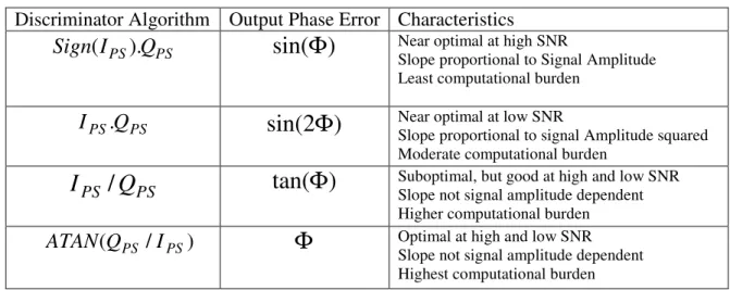
Table 3: Common Costas Loop discriminator used in GPS receivers (Ward 1996)
Discriminator Algorithm Output Phase Error Characteristics
PS PS
Q
I
Sign
(
).
sin(
Φ
)
Near optimal at high SNRSlope proportional to Signal Amplitude Least computational burden
PS PS
Q
I
.
sin(
2
Φ
)
Near optimal at low SNRSlope proportional to signal Amplitude squared Moderate computational burden
PS PS
Q
I
/
tan(
Φ
)
Suboptimal, but good at high and low SNR Slope not signal amplitude dependent Higher computational burden) / (QPS IPS
ATAN
Φ
Optimal at high and low SNRSlope not signal amplitude dependent Highest computational burden
Costas PLL loops can be used to detect the bits in satellite data message stream. The
PS
I
samples can be accumulated for the duration of one data bit (20 ms) and the sign ofthe result is the data bit. However, there will be a 180◦ phase ambiguity with Costas PLL
which will be corrected for during the frame synchronization process. This is done by
comparing the known preamble at the beginning of the each sub frame with the data bit
stream. If a match with the preamble is found, the bit stream will not be changed. If not,
an inverted pattern of preamble is check and if there is match, then the bit stream is
inverted as well.
Costas loops are sensitive to dynamic stress; however, they produce the most accurate
velocity measurements. Also, for a given signal power level, Costas PLL loops provide
make Costas PLL a very good candidate for GPS receivers. However, a well designed
GPS receiver starts tracking with the more robust FLL operated wide band, since it is less
sensitive to errors and noise. Then, gradually, it switches to a wideband PLL and finally
when the tracking is stable, to a narrow band PLL (Ward 1996).
Frequency Lock Loops:
A FLL is used to estimate the approximate frequency of the GPS signal. It is important
the FLL used in a GPS receiver be insensitive to 180◦ reversals in the I and Q signals.
Ward (1996) states it is usually easier to maintain frequency lock than phase lock when
data transition boundaries are unknown (example, during the initial signal acquisition).
This is due to the FLL discriminators being less sensitive to situations where some of the
I and Q signals do straddle the data bit transitions (Ward, 1996).
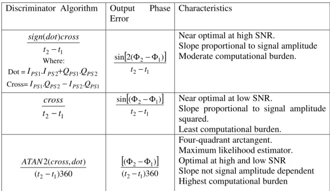
Table 4: Common GPS receiver FLL discriminators (Ward 1996)
Discriminator Algorithm Output Phase Error Characteristics 1 2 ) ( t t cross dot sign − Where: Dot =IPS1.IPS2+QPS1.QPS2 Cross=IPS1.QPS2−IPS2.QPS1
[
]
1 2 1 2 ) ( 2 sin t t − Φ − ΦNear optimal at high SNR.
Slope proportional to signal amplitude Moderate computational burden.
1 2 t t cross −
[
]
1 2 1 2 ) ( sin t t − Φ −Φ Near optimal at low SNR.
Slope proportional to signal amplitude squared.
Least computational burden.
360 ) ( ) , ( 2 1 2 t t dot cross ATAN −
[
]
360 ) ( ) ( 1 2 1 2 t t − Φ − Φ Four-quadrant arctangent. Maximum likelihood estimator. Optimal at high and low SNRSlope not signal amplitude dependent Highest computational burden
2.2.3.2 Code Tracking
The code tracking loop in the receiver is used to despread the incoming signal from the
data bits which are used to provide time of transmission measurements critical for range
measurements and subsequently a position solution. Code tracking loops are generally
characterized based on the pre-detection integrators, the code loop discriminators and
code loop filter. Table 5 summarizes some of the most common non-coherent delay lock
loops (DLL) and their characteristics.
Table 5 : Common Delay lock loop discriminators (Ward 1996)
Discriminator Algorithm Characteristic
∑
(IES −ILS)IPS +∑
(QES −QLS)QPS Dot product discriminator.Uses all 3 correlators.
Lowest computational burden.
For 0.5 chip spacing, produces nearly True error output within ±0.5chips.
∑
(
I
ES2+
Q
ES2)
−
∑
(
I
LS2+
Q
LS2)
Early minus late powerModerate computational burden
For 0.5 chip spacing, produces good tacking within ±0.5 chip of input error.
∑
(IES2 +QES2 ) −∑
(ILS2 +QLS2 ) Early minus late envelopeHigher computational burden
For 0.5 chip spacing, produces good tracking within ±0.5 chip of input error.
∑
∑
∑
∑
+ + + + − + 2 2 2 2 2 2 2 2 LS LS ES ES LS LS ES ES Q I Q I Q I QI Early minus late, normalized by early plus late envelope
Highest computational load
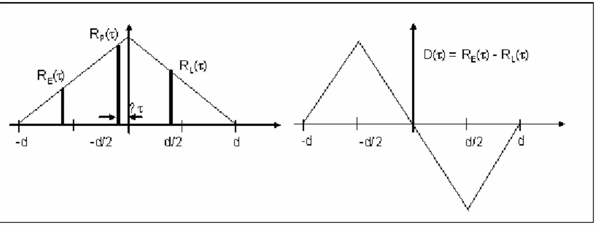
The correlation process mixes this input with the local early (E), punctual (P), and late
(L) code replicas in both the In-phase and Quadra-phase arms to get the IE, QE, IP, QP,
IL, and QL. Figure 13 shows the correlation power or the correlation envelope of the
thus, the IE, QE, IL, and QL are usually used in the DLL discriminator to obtain the
estimate of ∆τ.
Figure 13: Code mismatch early, prompt and late components
The result of the discriminators, energy in the early and late branches, which has been
differenced, is filtered, used to drive the NCO, which in turn clocks the PRN code
generator. The results indicate to the NCO that which branch, early or late, has more
power and whether the NCO needs to speed up or slow down the locally generated PRN
code (Ward 1996).
2.2.3.3 Loop Filters
The objective of loop filters is to reduce the noise so the receiver can better estimate the
desired signal. In this section, a very brief description of the filters used in typical GPS
receivers is given. For more information, refer to Ward 1996.
Table 6 summarizes the characteristics of some available loop filters. The order of the
is subject to acceleration dynamics, a third order loop for the PLL is selected since it is
insensitive to acceleration.
Table 6: Loop filter characteristics (Ward 1996) Loop Order Noise Bandwidth Typical filter value Steady-state Error Characteristics First
4
0ω
ω
0 0 25 . 0ω
= n B 0 ) (ω
dt dR Sensitive to velocityUsed in aided code loops/aided carrier loops
Unconditionally stable at all noise bandwidth Second 2 2 2 0
4
)
1
(
a
a
+
ω
ω
02 0 0 2ω =1.414ω a 0 53 . 0ω
= n B 2 0 2 2)
(
ω
dt
dR
Sensitive to acceleration Used in aided/unaided carrier loopsUnconditionally stable at all noise bandwidth Third ) 1 ( 4 ) ( 3 3 3 2 3 2 3 3 0 − − + b a b a b a ω 3 0 ω 2 0 3 0 3ω =1.1ω a 0 0 3ω =2.4ω b 0 7845 . 0 ω = n B 3 0 3 3
)
(
ω
dt
dR
Sensitive to jerk stress Used in unaided carrier loopsRemains stable at Bn−≤18Hz
2.2.4 Pseudo-range derivation
An ambiguity remains in the offset of the data bits after signal acquisition is carried out.
This is because the receiver has no timing information on the offset of the transmitted
data bits. The beginning of the C/A code is known but there is no timing information on
where the beginning of the data bit is (it has a length of 20 C/A code cycles). Failure in
detecting the right data bit will lead to failure in bit frame synchronization and failure in
recovering the navigation message from the signal.
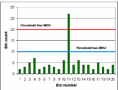
There are several methods that are used for data bit synchronization. One of the most
ms segments corresponding to the 20 C/A-code cycles. The receiver then tries to sense a
sign change between each of these C/A codes. If a sign change is sensed, a corresponding
histogram cell count is incremented until a count in one specific cell exceeds the other 19
bins by a pre-specified amount (Van Dierendonck 1996).
The algorithm operates as follows:
1. Create 20 cells and set a counter for each cell.
2. Initialize all counters to zero
3. Increment the appropriate cell counter when a sign change is observed.
4. Continue until one of the following conditions is met:
a. Two cell counts exceed threshold two
b. Loss of lock
c. One cell count exceeds threshold one
5. If
a. Condition (a) is met; conclude that the bit synchronization has failed. Go
back to step two.
b. Condition (b) is met; try to re-establish lock. And start over again.
c. (c) occurs, declare bit synchronization successful, and the C/A code
epoch count is reset to the correct value
The calculation of the thresholds is summarized briefly below. The more extensive
explanation can be found in (Van Dierendonck 1996).
The probability of making an error in determining a sign change at a desired signal of the
noise ratio (SNR) s as follows:
(
e)
e escP
P
P
=
2
1
−
(2.20) where(
)
[
S N T]
erfc Pe = ' 2 0 (2.21) and( )
∫
∞ −=
x ydy
e
x
erfc
2 22
1
'
π
(2.22)The number of entries,
N
bs, in a cell has a binominal distribution. OverT
bs seconds, theaverage number of sign changes (bit transitions) is 25Tbs so that in a correct cell
bs
T
NBS
1=
25
(2.23)and, in other cells
esc bs
bs
T
P
N
=
50
. (2.24)The thresholds, as well as the time interval
T
bs , are chosen to provide a good spreadbetween them at a desired SNR. Therefore, given
NBS
1, one needs to selectNBS
2 andbs
T
for a desired SNR so that the following inequality holds:(
esc)
bs esc esc bs bs T P P NBS T P T 3 50 1 50 25 − − ≥ 2 ≥ (2.25)The next step is frame synchronization. This is required in order to process the GPS data
and recover the navigation message. In the following few paragraphs, this process will be
briefly described.
As was discussed earlier in section 2.4, the GPS navigation message frame structure is
partitioned into five sub-frames. Each sub-frame is further subdivided into ten 30-bit
words with the two leading words being the telemetry (TLM) word and the handover
Several algorithms may be used for frame synchronization. Below, is the algorithm
employed in the software receiver used herein.
[1] Search for preamble or its inverted bit pattern.
[2] If found, a check is required to verify that the pattern is actually the preamble and it is
the beginning of a 30-bit word.
[3] Collect the following 22 bits and checking parity. If parity check does not pass, the
candidate preamble is discarded.
[4] There are also other legitimate patterns at the beginning of other words, so additional
checks are required. If the correct TLM word exists, the following word must be a HOW
word that contains a truncated Z-count. The first eight bits of this truncated Z-count can
also resemble a preamble.
[4] Check for parity on the HOW word. If it did not pass, restart the whole process again.
Test to verify the HOW word:
[5] If the HOW test passed, demodulation of the other words can start, and be stored in
memory.
[6]A final reliability check on the next preamble and the next Z-count confirms the frame
synchronization. This is to check if the preamble is in the right place and the Z-count
increments by one.
The next step is to calculate the pseudoranges. A pseudorange measurement is derived
based on the following equation
( )
[
( )
( )(
τ
)
]
where
)
(
t
t
u is the time of the signal arrival measured by the receiver clock.)
(
) (τ
−
t
t
s is the time of signal transmission by the satellite clock where it can bemeasured based on the Z count.
( )
(
)
chip code C/A of fraction chips code C/A whole of number codes C/A of number bits navigation of number count -Z + + + + = −τ
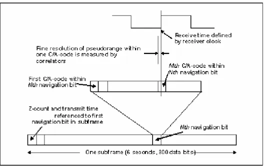
t t s (2.27)The process of pseudorange derivation is shown in figure 15 (Misra & Enge 2001). The
main goal is to establish the transmission time at the time of measurement. As shown, the
arrival time tu
( )
t kept by an inner clock is defined by a transition of the receiver clock. Ingeneral, these transitions occur sometime in the middle of a C/A code chip. The Z-count,
which is also included in the navigation message is a measure of Satellite time. Z-count
increments every 1.5 seconds, and the navigation message starts a new sub-frame every 6
Figure 15: Pseudorange derivation
Since the Z-count establishes satellite time at the beginning of each sub-frame, the
transmission time is the Z-count plus the whole number of C/A-code chips since the
beginning of the sub-frame. The elapsed time as stated in equation 2.27 is measured by
using the whole number of navigation bits, the whole number of C/A-codes since the
beginning of the current navigation bits, the number of whole C/A-code chips since the
beginning of the current code, the fraction of the current chip. The last two are measured
by the DLL and the rest are measured by counters in the bit synchronization and
sub-frame synchronization module in the receiver.
Later, all these pseudoranges are combined through the least-squares process to form a
navigation solution. An explanation of the theory of least-squares has been discussed in
Chapter 3
Real-time GPS Receiver Design
3.1 Computational Bottlenecks
The most computationally expensive task for a GPS receiver is the IF signal processing,
including Doppler removal and correlation with the local code. A receiver typically
needs to process GPS data acquired at a sampling rate of 2.5 MHz to 5 MHz for C/A
code. Additionally, the receiver must perform other operations such as tracking and
solution calculation in parallel with the signal processing operations. Although the latter
tasks typically run at a slow rate (0.1 to 10 Hz), the computational requirements must still
be considered, as they consume computational resources within the receiver.
Furthermore, the additional processing requirements for interfacing with an RF front-end
in real time must be considered. To satisfy these requirements, it is assumed for purposes
of this work that only 50% of the computer’s resources are available to the signal
processing component of the receiver. This is likely a conservative benchmark. To
illustrate the number of operations required, Table 7 shows the number of computations
needed in the receiver to process 1 ms of data with different sampling rates. The results
given are for a receiver tracking six satellites, the computation of three correlation values