32. Passage of particles through matter 1

32. PASSAGE OF PARTICLES THROUGH

MATTER . . . 2

32.1. Notation . . . 2

32.2. Electronic energy loss by heavy particles . . . 2

32.2.1. Moments and cross sections . . . 2

32.2.2. Maximum energy transfer in a single collision . . . 4

32.2.3. Stopping power at intermediate ener-gies . . . 5

32.2.4. Mean excitation energy . . . 6

32.2.5. Density effect . . . 7

32.2.6. Energy loss at low energies . . . 9

32.2.7. Energetic knock-on electrons (δ rays) . . . 10

32.2.8. Restricted energy loss rates for rela-tivistic ionizing particles . . . 10

32.2.9. Fluctuations in energy loss . . . 11

32.2.10. Energy loss in mixtures and com-pounds . . . 14

32.2.11. Ionization yields . . . 14

32.3. Multiple scattering through small angles . . . 15

32.4. Photon and electron interactions in mat-ter . . . 17

32.4.1. Collision energy losses by e± . . . 17

32.4.2. Radiation length . . . 18

32.4.3. Bremsstrahlung energy loss by e± . . . 19

32.4.4. Critical energy . . . 21

32.4.5. Energy loss by photons . . . 21

32.4.6. Bremsstrahlung and pair production at very high energies . . . 25

32.4.7. Photonuclear and electronuclear in-teractions at still higher energies . . . 26

32.5. Electromagnetic cascades . . . 27

32.6. Muon energy loss at high energy . . . 30

32.7. Cherenkov and transition radiation . . . 33

32.7.1. Optical Cherenkov radiation . . . 33

32.7.2. Coherent radio Cherenkov radiation . . . 34

32.7.3. Transition radiation . . . 35

32. PASSAGE OF PARTICLES THROUGH MATTER

This review covers the interactions of photons and electrically charged particles in matter, concentrating on energies of interest for high-energy physics and astrophysics and processes of interest for particle detectors (ionization, Cherenkov radiation, transition radiation). Much of the focus is on particles heavier than electrons (π±,p, etc.). Although the charge number z of the projectile is included in the equations, onlyz = 1 is discussed in detail. Muon radiative losses are discussed, as are photon/electron interactions at high to ultrahigh energies. Neutrons are not discussed. The notation and important numerical values are shown in Table 32.1.

32.1. Notation

32.2. Electronic energy loss by heavy particles

32.2.1. Moments and cross sections :

The electronic interactions of fast charged particles with speed v= βc occur in single collisions with energy losses W [1], leading to ionization, atomic, or collective excitation. Most frequently the energy losses are small (for 90% of all collisions the energy losses are less than 100 eV). In thin absorbers few collisions will take place and the total energy loss will show a large variance [1]; also see Sec. 32.2.9 below. For particles with charge

ze more massive than electrons (“heavy” particles), scattering from free electrons is adequately described by the Rutherford differential cross section [2],

dσR(W;β) dW = 2πr2_emec2z2 β2 (1₋β2W/Wmax) W2 , (32.1)

where Wmax is the maximum energy transfer possible in a single collision. But in matter electrons are not free. W must be finite and depends on atomic and bulk structure. For electrons bound in atoms Bethe [3] used “Born Theorie” to obtain the differential cross section

dσ_B(W;β)

dW =

dσ_R(W, β)

dW B(W) . (32.2)

Electronic binding is accounted for by the correction factor B(W). Examples of B(W) and dσ_B/dW can be seen in Figs. 5 and 6 of Ref. 1.

Bethe’s theory extends only to some energy above which atomic effects are not important. The free-electron cross section (Eq. (32.1)) can be used to extend the cross section to Wmax. At high energies σB is further modified by polarization of the medium,

and this “density effect,” discussed in Sec. 32.2.5, must also be included. Less important corrections are discussed below.

The mean number of collisions with energy loss between W and W +dW occurring in a distance δx is Neδx(dσ/dW)dW, where dσ(W;β)/dW contains all contributions. It is

convenient to define the moments

Mj(β) =Neδx Z

Wjdσ(W;β)

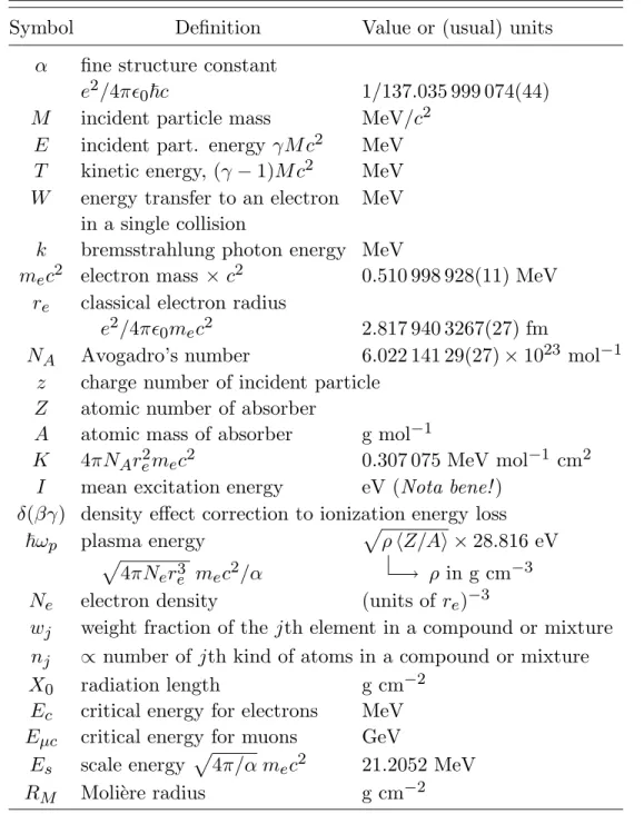
Table 32.1: Summary of variables used in this section. The kinematic variablesβ

andγ have their usual relativistic meanings.

Symbol Definition Value or (usual) units

α fine structure constant

e2/4πǫ0~_{c 1/137.035 999 074(44)}

M incident particle mass MeV/c2 E incident part. energy γM c2 MeV

T kinetic energy, (γ₋1)M c2 MeV

W energy transfer to an electron MeV in a single collision

k bremsstrahlung photon energy MeV

mec2 electron mass×c2 0.510 998 928(11) MeV

re classical electron radius

e2/4πǫ0mec2 2.817 940 3267(27) fm

N_A Avogadro’s number 6.022 141 29(27)_×1023 mol−1

z charge number of incident particle

Z atomic number of absorber

A atomic mass of absorber g mol−1

K 4πN_Ar_e2mec2 0.307 075 MeV mol−1 cm2

I mean excitation energy eV (Nota bene!)

δ(βγ) density effect correction to ionization energy loss ~_{ωp plasma energy} p_{ρhZ/Ai ×28.816 eV}

p

4πNer3e mec2/α |−→ ρ in g cm−3

Ne electron density (units of re)−3

wj weight fraction of the jth element in a compound or mixture

nj ∝ number ofjth kind of atoms in a compound or mixture

X0 radiation length g cm−2

Ec critical energy for electrons MeV

Eµc critical energy for muons GeV

Es scale energy p4π/α mec2 21.2052 MeV

RM Moli`ere radius g cm−2

so that M0 is the mean number of collisions in δx, M1 is the mean energy loss in δx, (M2₋M1)2 is the variance, etc. The number of collisions is Poisson-distributed with mean M0. Ne is either measured in electrons/g (Ne = NAZ/A) or electrons/cm3

(Ne =NAρZ/A). The former is used throughout this chapter, since quantities of interest

Muon momentum

10 100

Stopping power [MeV cm

2

/g]

βγ

[MeV/c]

[GeV/c]

[TeV/c]

µ

µ

on Cu

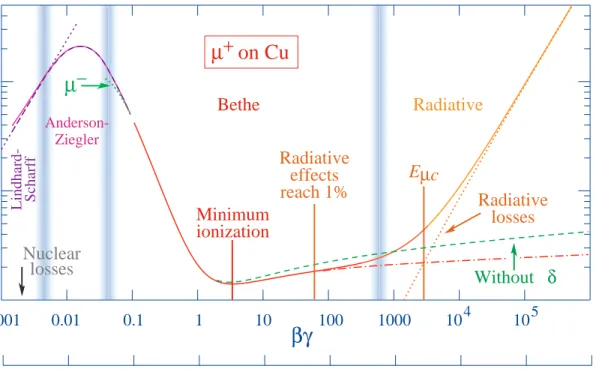
Fig. 32.1: Stopping power (= _h−dE/dx_i) for positive muons in copper as a function of

βγ =p/M c over nine orders of magnitude in momentum (12 orders of magnitude in kinetic energy). Solid curves indicate the total stopping power. Data below the break at βγ _≈0.1 are taken from ICRU 49 [4], and data at higher energies are from Ref. 5. Vertical bands indicate boundaries between different approximations discussed in the text. The short dotted lines labeled “µ−” illustrate the “Barkas effect,” the dependence of stopping power on projectile charge at very low energies [6]. dE/dx in the radiative region is not simply a function of β.

32.2.2. Maximum energy transfer in a single collision : For a particle with mass

M,

Wmax = 2mec 2_β2_γ2

1 + 2γme/M + (me/M)2 . (32.4)

In older references [2,8] the “low-energy” approximation Wmax = 2mec2β2γ2, valid for

2γme ≪M, is often implicit. For a pion in copper, the error thus introduced into dE/dx

is greater than 6% at 100 GeV. For 2γme ≫M, Wmax =M c2β2γ.

At energies of order 100 GeV, the maximum 4-momentum transfer to the electron can exceed 1 GeV/c, where hadronic structure effects significantly modify the cross sections. This problem has been investigated by J.D. Jackson [9], who concluded that for hadrons (but not for large nuclei) corrections to dE/dx are negligible below energies where radiative effects dominate. While the cross section for rare hard collisions is modified, the average stopping power, dominated by many softer collisions, is almost unchanged.

32.2.3. Stopping power at intermediate energies :

The mean rate of energy loss by moderately relativistic charged heavy particles,

M1/δx, is well-described by the “Bethe equation,”

¿ −dE_dx À =Kz2Z A 1 β2 · 1 2ln 2mec2β2γ2Wmax I2 −β 2 − δ(βγ₂ ) ¸ . (32.5) It describes the mean rate of energy loss in the region 0.1<_∼βγ <_∼1000 for intermediate-Z

materials with an accuracy of a few %. With the symbol definitions and values given in Table 32.1, the units are MeV g−1cm2. Wmax is defined in Sec. 32.2.2. At the lower limit the projectile velocity becomes comparable to atomic electron “velocities” (Sec. 32.2.6), and at the upper limit radiative effects begin to be important (Sec. 32.6). Both limits are

Z dependent. A minor dependence on M at the highest energies is introduced through

Wmax, but for all practical purposes _hdE/dx_iin a given material is a function of β alone. Few concepts in high-energy physics are as misused as _hdE/dx_i. The main problem is that the mean is weighted by very rare events with large single-collision energy deposits. Even with samples of hundreds of events a dependable value for the mean energy loss cannot be obtained. Far better and more easily measured is the most probable energy loss, discussed in Sec. 32.2.9. The most probable energy loss in a detector is considerably below the mean given by the Bethe equation.

In a TPC (Sec. 33.6.5), the mean of 50%–70% of the samples with the smallest signals is often used as an estimator.

Although it must be used with cautions and caveats,_hdE/dx_ias described in Eq. (32.5) still forms the basis of much of our understanding of energy loss by charged particles. Extensive tables are available[4,5, pdg.lbl.gov/AtomicNuclearProperties/].

For heavy projectiles, like ions, additional terms are required to account for higher-order photon coupling to the target, and to account for the finite size of the target radius. These can change dE/dx by a factor of two or more for the heaviest nuclei in certain kinematic regimes [7].

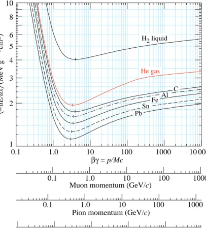
The function as computed for muons on copper is shown as the “Bethe” region of Fig. 32.1. Mean energy loss behavior below this region is discussed in Sec. 32.2.6, and the radiative effects at high energy are discussed in Sec. 32.6. Only in the Bethe region is it a function of β alone; the mass dependence is more complicated elsewhere. The stopping power in several other materials is shown in Fig. 32.2. Except in hydrogen, particles with the same velocity have similar rates of energy loss in different materials, although there is a slow decrease in the rate of energy loss with increasing Z. The qualitative behavior difference at high energies between a gas (He in the figure) and the other materials shown in the figure is due to the density-effect correction, δ(βγ), discussed in Sec. 32.2.5. The stopping power functions are characterized by broad minima whose position drops from

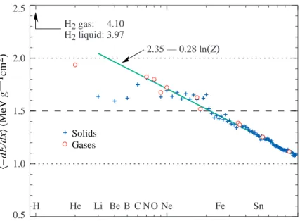
βγ = 3.5 to 3.0 as Z goes from 7 to 100. The values of minimum ionization as a function of atomic number are shown in Fig. 32.3.

In practical cases, most relativistic particles (e.g., cosmic-ray muons) have mean energy loss rates close to the minimum; they are “minimum-ionizing particles,” or mip’s.

Eq. (32.5) may be integrated to find the total (or partial) “continuous slowing-down approximation” (CSDA) rangeR for a particle which loses energy only through ionization and atomic excitation. Since dE/dx depends only on β, R/M is a function of E/M or

1 2 3 4 5 6 8 10 1.0 10 100 1000 10 000 0.1

Pion momentum (GeV/c)

Proton momentum (GeV/c)

1.0 10 100 1000

0.1

1.0 10 100 1000

0.1

βγ=p/Mc

Muon momentum (GeV/c)

H₂ liquid He gas C Al Fe Sn Pb 〈 – dE/dx 〉 (MeV g —1 cm 2) 1.0 10 100 1000 10 000 0.1

Figure 32.2: Mean energy loss rate in liquid (bubble chamber) hydrogen, gaseous helium, carbon, aluminum, iron, tin, and lead. Radiative effects, relevant for muons and pions, are not included. These become significant for muons in iron for

βγ >_∼1000, and at lower momenta for muons in higher-Z absorbers. See Fig. 32.23.

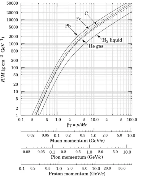
pc/M. In practice, range is a useful concept only for low-energy hadrons (R <_∼λI, where

λI is the nuclear interaction length), and for muons below a few hundred GeV (above

which radiative effects dominate). R/M as a function of βγ = p/M c is shown for a variety of materials in Fig. 32.4.

The mass scaling of dE/dx and range is valid for the electronic losses described by the Bethe equation, but not for radiative losses, relevant only for muons and pions.

32.2.4. Mean excitation energy : “The determination of the mean excitation energy is the principal non-trivial task in the evaluation of the Bethe stopping-power formula” [10]. Recommended values have varied substantially with time. Estimates based on experimental stopping-power measurements for protons, deuterons, and alpha particles and on oscillator-strength distributions and dielectric-response functions were given in ICRU 49 [4]. See also ICRU 37 [11]. These values, shown in Fig. 32.5, have since been widely used. Machine-readable versions can also be found [12].

0.5 1.0 1.5 2.0 2.5 1 2 5 10 20 50 100 Z H He Li Be B C NO Ne Fe Sn Solids Gases H2 gas: 4.10 H2 liquid: 3.97 2.35 — 0.28 ln(Z) 〈 – dE/dx 〉 (MeV g —1 cm 2)

Figure 32.3: Stopping power at minimum ionization for the chemical elements. The straight line is fitted for Z >6. A simple functional dependence on Z is not to be expected, since_h−dE/dx_i also depends on other variables.

32.2.5. Density effect : As the particle energy increases, its electric field flattens and extends, so that the distant-collision contribution to Eq. (32.5) increases as lnβγ. However, real media become polarized, limiting the field extension and effectively truncating this part of the logarithmic rise [2–8,15–16]. At very high energies,

δ/2_→ ln(~_{ωp/I) + lnβγ−1/2 , (32.6)} where δ(βγ)/2 is the density effect correction introduced in Eq. (32.5) and ~_{ωp is the} plasma energy defined in Table 32.1. A comparison with Eq. (32.5) shows that _|dE/dx_|

then grows as lnβγ rather than lnβ2γ2, and that the mean excitation energyI is replaced by the plasma energy ~_{ωp. The ionization stopping power as calculated with and without} the density effect correction is shown in Fig. 32.1. Since the plasma frequency scales as the square root of the electron density, the correction is much larger for a liquid or solid than for a gas, as is illustrated by the examples in Fig. 32.2.

The density effect correction is usually computed using Sternheimer’s parameteriza-tion [15]: δ(βγ) =        2(ln 10)x₋C ifx_≥x1; 2(ln 10)x₋C+a(x1₋x)k ifx0 _≤x < x1; 0 ifx < x0 (nonconductors); δ0102(x−x0) ifx < x0 (conductors) (32.7)

Here x = log₁₀η = log₁₀(p/M c). C (the negative of the C used in Ref. 15) is obtained by equating the high-energy case of Eq. (32.7) with the limit given in Eq. (32.6). The other parameters are adjusted to give a best fit to the results of detailed calculations for momenta below M cexp(x1). Parameters for elements and nearly 200 compounds and

0.05 0.1

0.02 0.2 0.5 1.0 2.0 5.0 10.0

Pion momentum (GeV/c)

0.1 0.2 0.5 1.0 2.0 5.0 10.0 20.0 50.0 Proton momentum (GeV/c)

0.05

0.02 _0.1 0.2 0.5 _1.0 2.0 5.0 _10.0

Muon momentum (GeV/c)

βγ = p/Mc 1 2 5 10 20 50 100 200 500 1000 2000 5000 10000 20000 50000 R / M (g cm − 2 GeV − 1) 0.1 2 5 1.0 2 5 10.0 2 5 100.0 H₂ liquid He gas Pb Fe C

Figure 32.4: Range of heavy charged particles in liquid (bubble chamber) hydrogen, helium gas, carbon, iron, and lead. For example: For a K+ whose momentum is 700 MeV/c, βγ = 1.42. For lead we read R/M _≈ 396, and so the range is 195 g cm−2 (17 cm).

finding the coefficients for nontabulated materials is given by Sternheimer and Peierls [17], and is summarized in Ref. 5.

The remaining relativistic rise comes from the β2γ growth of Wmax, which in turn is due to (rare) large energy transfers to a few electrons. When these events are excluded, the energy deposit in an absorbing layer approaches a constant value, the Fermi plateau (see Sec. 32.2.8 below). At even higher energies (e.g., >332 GeV for muons in iron, and at a considerably higher energy for protons in iron), radiative effects are more important than ionization losses. These are especially relevant for high-energy muons, as discussed in Sec. 32.6.

0 10 20 30 40 50 60 70 80 90 100 8 10 12 14 16 18 20 22 Iadj / Z (eV) Z

Barkas & Berger 1964 Bichsel 1992 ICRU 37 (1984)

(interpolated values are not marked with points)

Figure 32.5: Mean excitation energies (divided by Z) as adopted by the ICRU [11]. Those based on experimental measurements are shown by symbols with error flags; the interpolated values are simply joined. The grey point is for liquid H2; the black

point at 19.2 eV is for H2 gas. The open circles show more recent determinations by

Bichsel [13]. The dash-dotted curve is from the approximate formula of Barkas [14] used in early editions of thisReview.

32.2.6. Energy loss at low energies : Shell corrections C/Z must be included in the square brackets of of Eq. (32.5) [4,11,13,14] to correct for atomic binding having been neglected in calculating some of the contributions to Eq. (32.5). The Barkas form [14] was used in generating Fig. 32.1. For copper it contributes about 1% at βγ = 0.3 (kinetic energy 6 MeV for a pion), and the correction decreases very rapidly with increasing energy.

Equation 32.2, and therefore Eq. (32.5), are based on a first-order Born approximation. Higher-order corrections, again important only at lower energies, are normally included by adding the “Bloch correction” z2L2(β) inside the square brackets (Eq.(2.5) in [4]) .

An additional “Barkas correction” zL1(β) reduces the stopping power for a negative particle below that for a positive particle with the same mass and velocity. In a 1956 paper, Barkas et al. noted that negative pions had a longer range than positive pions [6]. The effect has been measured for a number of negative/positive particle pairs, including a detailed study with antiprotons [18].

A detailed discussion of low-energy corrections to the Bethe formula is given in ICRU 49 [4]. When the corrections are properly included, the Bethe treatment is accurate to about 1% down to β _≈0.05, or about 1 MeV for protons.

For 0.01 < β < 0.05, there is no satisfactory theory. For protons, one usually relies on the phenomenological fitting formulae developed by Andersen and Ziegler [4,19]. As tabulated in ICRU 49 [4], the nuclear plus electronic proton stopping power in copper is 113 MeV cm2g−1 at T = 10 keV (βγ = 0.005), rises to a maximum of 210 MeV cm2g−1 atT _≈120 keV (βγ = 0.016), then falls to 118 MeV cm2g−1 atT = 1 MeV (βγ = 0.046).

Above 0.5–1.0 MeV the corrected Bethe theory is adequate.

For particles moving more slowly than _≈ 0.01c (more or less the velocity of the outer atomic electrons), Lindhard has been quite successful in describing electronic stopping power, which is proportional to β [20]. Finally, we note that at even lower energies,

e.g., for protons of less than several hundred eV, non-ionizing nuclear recoil energy loss dominates the total energy loss [4,20,21].

32.2.7. Energetic knock-on electrons (δ _{rays): The distribution of secondary}

electrons with kinetic energies T _≫I is [2]

d2N dT dx = 1 2 Kz 2Z A 1 β2 F(T) T2 (32.8)

for I _≪ T _≤ Wmax, where Wmax is given by Eq. (32.4). Here β is the velocity of the primary particle. The factor F is spin-dependent, but is about unity for T _≪ Wmax.

For spin-0 particles F(T) = (1₋β2T /Wmax); forms for spins 1/2 and 1 are also given by Rossi [2]( Sec. 2.3, Eqns. 7 and 8). Additional formulae are given in Ref. 22. Equation (32.8) is inaccurate for T close to I [23].

δ rays of even modest energy are rare. For a β _≈ 1 particle, for example, on average only one collision withTe >10 keV will occur along a path length of 90 cm of Ar gas [1].

A δ ray with kinetic energy Te and corresponding momentum pe is produced at an

angle θ given by

cosθ= (Te/pe)(pmax/Wmax) , (32.9)

where pmax is the momentum of an electron with the maximum possible energy transfer

Wmax.

32.2.8. Restricted energy loss rates for relativistic ionizing particles : Further insight can be obtained by examining the mean energy deposit by an ionizing particle when energy transfers are restricted to T _≤ Wcut _≤ Wmax. The restricted energy loss rate is −dE dx ¯ ¯ ¯ ¯ T <W_cut =Kz2Z A 1 β2 · 1 2ln 2mec2β2γ2Wcut I2 −β 2 2 µ 1 + Wcut Wmax ¶ − δ₂ ¸ . (32.10)

This form approaches the normal Bethe function (Eq. (32.5)) as Wcut → Wmax. It

can be verified that the difference between Eq. (32.5) and Eq. (32.10) is equal to

RW_max Wcut T(d

2_{N/dT dx)dT, whered}2_{N/dT dx is given by Eq. (32.8).}

Since Wcut replaces Wmax in the argument of the logarithmic term of Eq. (32.5), the

βγ term producing the relativistic rise in the close-collision part of dE/dx is replaced by a constant, and _|dE/dx_|T <W_cut approaches the constant “Fermi plateau.” (The density

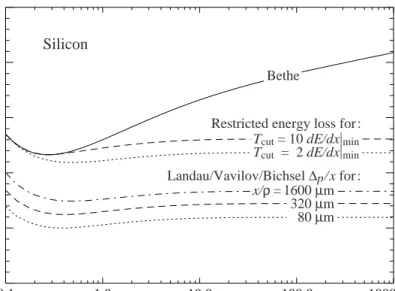
effect correctionδ eliminates the explicitβγ dependence produced by the distant-collision contribution.) This behavior is illustrated in Fig. 32.6, where restricted loss rates for two examples of Wcut are shown in comparison with the full Bethe dE/dx and the

Landau/Vavilov/Bichsel ∆p/x for :

Bethe

Tcut = 10 dE/dx|min

Tcut = 2 dE/dx|min Restricted energy loss for :

0.1 1.0 10.0 100.0 1000.0 1.0 1.5 0.5 2.0 2.5 3.0 MeV g − 1 cm 2 (Electonic loses only)

Muon kinetic energy (GeV) Silicon

x/ρ = 1600 µm 320 µm 80 µm

Figure 32.6: BethedE/dx, two examples of restricted energy loss, and the Landau most probable energy per unit thickness in silicon. The change of ∆p/x with

thickness x illustrates its alnx+b dependence. Minimum ionization (dE/dx_|min)

is 1.664 MeV g−1cm2. Radiative losses are excluded. The incident particles are muons.

“Restricted energy loss” is cut at the total mean energy, not the single-collision energy above Wcut It is of limited use. The most probable energy loss, discussed in the next Section, is far more useful in situations where single-particle energy loss is observed.

32.2.9. Fluctuations in energy loss : For detectors of moderate thickness x (e.g.

scintillators or LAr cells),* the energy loss probability distribution f(∆;βγ, x) is ade-quately described by the highly-skewed Landau (or Landau-Vavilov) distribution [24,25]. The most probable energy loss is [26]†

∆p =ξ · ln2mc 2_β2_γ2 I + ln ξ I +j−β 2 −δ(βγ) ¸ , (32.11) where ξ = (K/2)_hZ/A_i(x/β2) MeV for a detector with a thickness x in g cm−2, and

j = 0.200 [26]. ‡ While dE/dx is independent of thickness, ∆p/x scales asalnx+b. The

density correction δ(βγ) was not included in Landau’s or Vavilov’s work, but it was later * G <_∼ 0.05–0.1, where G is given by Rossi [Ref. 2, Eq. 2.7(10)]. It is Vavilov’s κ [25]. It is proportional to the absorber’s thickness, and as such parameterizes the constants describing the Landau distribution. These are fairly insensitive to thickness for G <_∼ 0.1, the case for most detectors.

† _{Practical calculations can be expedited by using the tables ofδandβ from the text}

ver-sions of the muon energy loss tables to be found atpdg.lbl.gov/AtomicNuclearProperties.

‡ _{Rossi [2], Talman [27], and others give somewhat different values for j. The most}

included by Bichsel [26]. The high-energy behavior ofδ(βγ) (Eq. (32.6)) is such that ∆p −→ βγ>_∼100 ξ · ln 2mc 2_ξ (~_ωp)2 +j ¸ . (32.12)

Thus the Landau-Vavilov most probable energy loss, like the restricted energy loss, reaches a Fermi plateau. The Bethe dE/dx and Landau-Vavilov-Bichsel ∆p/x in silicon

are shown as a function of muon energy in Fig. 32.6. The energy deposit in the 1600 µm case is roughly the same as in a 3 mm thick plastic scintillator.

f ( Δ ) [M eV − 1 ]

Electronic energy loss Δ [MeV] Energy loss [MeV cm2_/g]

150 100 50 0 0.4 0.5 0.6 0.7 0.8 0.9 1.0 0.8 1.0 0.6 0.4 0.2 0.0 Mj ( Δ )/ Mj ( ∞ ) Landau-Vavilov

Bichsel (Bethe-Fano theory)

Δp Δ fwhm M₀(Δ)/M₀(∞) Μ₁(Δ)/Μ₁(∞) 10 GeV muon 1.7 mm Si 1.2 1.4 1.6 1.8 2.0 2.2 2.4

< >

Figure 32.7: Electronic energy deposit distribution for a 10 GeV muon traversing 1.7 mm of silicon, the stopping power equivalent of about 0.3 cm of PVC scintillator [1,13,28]. The Landau-Vavilov function (dot-dashed) uses a Rutherford cross section without atomic binding corrections but with a kinetic energy transfer limit of Wmax. The solid curve was calculated using Bethe-Fano theory. M0(∆)

and M1(∆) are the cumulative 0th moment (mean number of collisions) and 1st moment (mean energy loss) in crossing the silicon. (See Sec. 32.2.1. The fwhm of the Landau-Vavilov function is about 4ξ for detectors of moderate thickness. ∆p

is the most probable energy loss, and _h∆_i divided by the thickness is the Bethe hdE/dx_i.

The distribution function for the energy deposit by a 10 GeV muon going through a detector of about this thickness is shown in Fig. 32.7. In this case the most probable energy loss is 62% of the mean (M1(h∆i)/M1(∞)). Folding in experimental resolution

displaces the peak of the distribution, usually toward a higher value. 90% of the collisions (M1(h∆i)/M1(∞)) contribute to energy deposits below the mean. It is the very rare

high-energy-transfer collisions, extending to Wmax at several GeV, that drives the mean

into the tail of the distribution. The large weight of these rare events makes the mean of an experimental distribution consisting of a few hundred events subject to large fluctuations and sensitive to cuts. The mean of the energy loss given by the Bethe

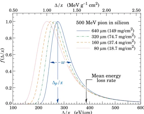
100 200 300 400 500 600 0.0 0.2 0.4 0.6 0.8 1.0 0.50 1.00 1.50 2.00 2.50 640 µm (149 mg/cm2₎ 320 µm (74.7 mg/cm2₎ 160 µm (37.4 mg/cm2₎ 80 µm (18.7 mg/cm2)

500 MeV pion in silicon

Mean energy loss rate w f ( ∆ /x ) ∆/x (eV/µm) ∆p/x ∆/x (MeV g−1 cm2)

Figure 32.8: Straggling functions in silicon for 500 MeV pions, normalized to unity at the most probable valueδp/x. The width w is the full width at half maximum. equation, Eq. (32.5), is thus ill-defined experimentally and is not useful for describing energy loss by single particles.♮ It rises as lnγ because Wmax increases as γ at high energies. The most probable energy loss should be used.

A practical example: For muons traversing 0.25 inches of PVT plastic scintillator, the ratio of the most probable E loss rate to the mean loss rate via the Bethe equation is [0.69,0.57,0.49,0.42,0.38] for Tµ = [0.01,0.1,1,10,100] GeV. Radiative losses add less

than 0.5% to the total mean energy deposit at 10 GeV, but add 7% at 100 GeV. The most probable E loss rate rises slightly beyond the minimum ionization energy, then is essentially constant.

The Landau distribution fails to describe energy loss in thin absorbers such as gas TPC cells [1] and Si detectors [26], as shown clearly in Fig. 1 of Ref. 1 for an argon-filled TPC cell. Also see Talman [27]. While ∆p/x may be calculated adequately with Eq. (32.11),

the distributions are significantly wider than the Landau width w= 4ξ [Ref. 26, Fig. 15]. Examples for 500 MeV pions incident on thin silicon detectors are shown in Fig. 32.8. For very thick absorbers the distribution is less skewed but never approaches a Gaussian.

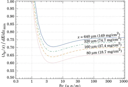
The most probable energy loss, scaled to the mean loss at minimum ionization, is shown in Fig. 32.9 for several silicon detector thicknesses.

1 3 0.3 10 30 100 300 1000 βγ (= p/m) 0.50 0.55 0.60 0.65 0.70 0.75 0.80 0.85 0.90 0.95 1.00 ( ∆p /x )

/

Figure 32.9: Most probable energy loss in silicon, scaled to the mean loss of a minimum ionizing particle, 388 eV/µm (1.66 MeV g−1cm2).

32.2.10. Energy loss in mixtures and compounds : A mixture or compound can be thought of as made up of thin layers of pure elements in the right proportion (Bragg additivity). In this case,

¿ dE dx À =Xwj ¿ dE dx À j , (32.13)

where dE/dx_|j is the mean rate of energy loss (in MeV g cm−2) in the jth element.

Eq. (32.5) can be inserted into Eq. (32.13) to find expressions for _hZ/A_i, _hI_i, and _hδ_i; for example, _hZ/A_i = P

wjZj/Aj = PnjZj/PnjAj. However, hIi as defined this way is

an underestimate, because in a compound electrons are more tightly bound than in the free elements, and _hδ_i as calculated this way has little relevance, because it is the electron density that matters. If possible, one uses the tables given in Refs. 16 and 29, that include effective excitation energies and interpolation coefficients for calculating the density effect correction for the chemical elements and nearly 200 mixtures and compounds. Otherwise, use the recipe for δ given in Ref. 5 and 17, and calculate _hI_i following the discussion in Ref. 10. (Note the “13%” rule!)

32.2.11. Ionization yields: Physicists frequently relate total energy loss to the number of ion pairs produced near the particle’s track. This relation becomes complicated for relativistic particles due to the wandering of energetic knock-on electrons whose ranges exceed the dimensions of the fiducial volume. For a qualitative appraisal of the nonlocality of energy deposition in various media by such modestly energetic knock-on electrons, see Ref. 30. The mean local energy dissipation per local ion pair produced, W, while essentially constant for relativistic particles, increases at slow particle speeds [31]. For gases, W can be surprisingly sensitive to trace amounts of various contaminants [31]. Furthermore, ionization yields in practical cases may be greatly influenced by such factors

as subsequent recombination [32].

32.3. Multiple scattering through small angles

A charged particle traversing a medium is deflected by many small-angle scatters. Most of this deflection is due to Coulomb scattering from nuclei as described by the Rutherford cross section. (However, for hadronic projectiles, the strong interactions also contribute to multiple scattering.) For many small-angle scatters the net scattering and displacement distributions are Gaussian via the central limit theorem. Less frequent “hard” scatters produce non-Gaussian tails. These Coulomb scattering distributions are well-represented by the theory of Moli`ere [34]. Accessible discussions are given by Rossi [2] and Jackson [33], and exhaustive reviews have been published by Scott [35] and Motz et al. [36]. Experimental measurements have been published by Bichsel [37]( low energy protons) and by Shen et al.[38]( relativistic pions, kaons, and protons).*

If we define θ0 =θrmsplane= 1 √ 2θ rms space , (32.14)

then it is sufficient for many applications to use a Gaussian approximation for the central 98% of the projected angular distribution, with an rms width given by [39,40]

θ0 = 13.6 MeV βcp z p x/X0 h 1 + 0.038 ln(x/X0) i . (32.15) Here p,βc, and z are the momentum, velocity, and charge number of the incident particle, and x/X0 is the thickness of the scattering medium in radiation lengths (defined below).

This value of θ0 is from a fit to Moli`ere distribution for singly charged particles with

β = 1 for all Z, and is accurate to 11% or better for 10−3< x/X0 <100.

Eq. (32.15) describes scattering from a single material, while the usual problem involves the multiple scattering of a particle traversing many different layers and mixtures. Since it is from a fit to a Moli`ere distribution, it is incorrect to add the individualθ0 contributions

in quadrature; the result is systematically too small. It is much more accurate to apply Eq. (32.15) once, after findingx andX0 for the combined scatterer.

The nonprojected (space) and projected (plane) angular distributions are given approximately by [34] 1 2π θ₀2 exp     − θ_space2 2θ2₀     dΩ , (32.16) 1 √ 2π θ0 exp      − θ2_plane 2θ2₀       dθ_plane , (32.17) whereθ is the deflection angle. In this approximation, θ_space2 _≈(θ2_plane,x+θ2_plane,y), where the x and y axes are orthogonal to the direction of motion, and dΩ_≈ dθplane,xdθplane,y.

Deflections into θplane,x and θplane,y are independent and identically distributed.

* Shen et al.’s measurements show that Bethe’s simpler methods of including atomic electron effects agrees better with experiment than does Scott’s treatment.

x

s_plane yplane

Ψ_plane

θ_plane

x /2

Figure 32.10: Quantities used to describe multiple Coulomb scattering. The particle is incident in the plane of the figure.

Fig. 32.10 shows these and other quantities sometimes used to describe multiple Coulomb scattering. They are

ψrms_plane= √1 3θ rms plane = 1 √ 3θ0 , (32.18) yrms_plane= _√1 3x θ rms plane = 1 √ 3x θ0 , (32.19) srms_plane= 1 4√3x θ rms plane= 1 4√3x θ0 . (32.20)

All the quantitative estimates in this section apply only in the limit of smallθrms_plane and in the absence of large-angle scatters. The random variabless,ψ,y, andθ in a given plane are correlated. Obviously, y _≈ xψ. In addition, y and θ have the correlation coefficient

ρyθ = √3/2≈ 0.87. For Monte Carlo generation of a joint (yplane, θplane) distribution,

or for other calculations, it may be most convenient to work with independent Gaussian random variables (z1, z2) with mean zero and variance one, and then set

y_plane=z1x θ0(1−ρ2_yθ)1/2/√3 +z2ρyθx θ0/√3 (32.21)

=z1x θ0/

√

12 +z2x θ0/2 ; (32.22)

θplane=z2θ0 . (32.23)

Note that the second term for yplane equals x θplane/2 and represents the displacement

that would have occurred had the deflection θ_plane all occurred at the single point x/2. For heavy ions the multiple Coulomb scattering has been measured and compared with various theoretical distributions [41].

32.4. Photon and electron interactions in matter

At low energies electrons and positrons primarily lose energy by ionization, although other processes (Møller scattering, Bhabha scattering, e+ annihilation) contribute, as shown in Fig. 32.11. While ionization loss rates rise logarithmically with energy, bremsstrahlung losses rise nearly linearly (fractional loss is nearly independent of energy), and dominates above the critical energy (Sec. 32.4.4 below), a few tens of MeV in most materials

32.4.1. Collision energy losses by e± _{: Stopping power differs somewhat for electrons}

and positrons, and both differ from stopping power for heavy particles because of the kinematics, spin, charge, and the identity of the incident electron with the electrons that it ionizes. Complete discussions and tables can be found in Refs. 10, 11, and 29.

For electrons, large energy transfers to atomic electrons (taken as free) are described by the Møller cross section. From Eq. (32.4), the maximum energy transfer in a single collision should be the entire kinetic energy, Wmax = mec2(γ −1), but because the

particles are identical, the maximum is half this, Wmax/2. (The results are the same if

the transferred energy is ǫ or if the transferred energy isWmax₋ǫ. The stopping power is by convention calculated for the faster of the two emerging electrons.) The first moment of the Møller cross section [22]( divided bydx) is the stopping power:

¿ −dE_dx À =1 2K Z A 1 β2 · ln mec 2_β2_γ2_{m ec2(γ−1)/2} I2 +(1₋β2)₋ 2γ−1 γ2 ln 2 + 1 8 µ γ₋1 γ ¶2 −δ # (32.24) The logarithmic term can be compared with the logarithmic term in the Bethe equation (Eq. (32.2)) by substituting Wmax =mec2(γ−1)/2. The two forms differ by ln 2.

Electron-positron scattering is described by the fairly complicated Bhabha cross section [22]. There is no identical particle problem, so Wmax =mec2(γ −1). The first

moment of the Bhabha equation yields

¿ −dE dx À =1 2K Z A 1 β2 · lnmec 2_β2_γ2_{m ec2(γ−1)} 2I2 +2 ln 2₋ β 2 12 µ 23 + 14 γ+ 1 + 10 (γ + 1)2 + 4 (γ + 1)3 ¶ −δ ¸ . (32.25) Following ICRU 37 [11], the density effect correction δ has been added to Uehling’s equations [22] in both cases.

For heavy particles, shell corrections were developed assuming that the projectile is equivalent to a perturbing potential whose center moves with constant velocity. This assumption has no sound theoretical basis for electrons. The authors of ICRU 37 [11] estimated the possible error in omitting it by assuming the correction was twice as great as for a proton of the same velocity. At T = 10 keV, the error was estimated to be _≈2% for water, _≈9% for Cu, and _≈21% for Au.

As shown in Fig. 32.11, stopping powers for e−, e+, and heavy particles are not dramatically different. In silicon, the minimum value for electrons is 1.50 MeV cm2/g (at

γ = 3.3); for positrons, 1.46 MeV cm2/g (atγ = 3.7), and for muons, 1.66 MeV cm2/g (at

γ = 3.58).

32.4.2. Radiation length : High-energy electrons predominantly lose energy in matter by bremsstrahlung, and high-energy photons by e+e− pair production. The characteristic amount of matter traversed for these related interactions is called the radiation length X0, usually measured in g cm−2. It is both (a) the mean distance over

which a high-energy electron loses all but 1/e of its energy by bremsstrahlung, and (b) 7₉ of the mean free path for pair production by a high-energy photon [42]. It is also the appropriate scale length for describing high-energy electromagnetic cascades. X0 has

been calculated and tabulated by Y.S. Tsai [43]: 1 X0 = 4αr 2 e NA A n Z2£ Lrad−f(Z)¤+Z L′rad o . (32.26) For A = 1 g mol−1, 4αr_e2N_A/A = (716.408 g cm−2)−1. L_rad and L′_rad are given in Table 32.2. The function f(Z) is an infinite sum, but for elements up to uranium can be represented to 4-place accuracy by

f(Z) =a2 · (1 +a2)−1+ 0.20206 −0.0369a2+ 0.0083a4₋0.002a6 ¸ , (32.27) where a=αZ [44].

Table 32.2: Tsai’s Lrad and L′_rad, for use in calculating the radiation length in an

element using Eq. (32.26).

Element Z Lrad L′_rad

H 1 5.31 6.144

He 2 4.79 5.621

Li 3 4.74 5.805

Be 4 4.71 5.924

Others >4 ln(184.15Z−1/3) ln(1194Z−2/3)

The radiation length in a mixture or compound may be approximated by

1/X0=Xwj/Xj , (32.28)

Figure 32.11: Fractional energy loss per radiation length in lead as a function of electron or positron energy. Electron (positron) scattering is considered as ionization when the energy loss per collision is below 0.255 MeV, and as Møller (Bhabha) scattering when it is above. Adapted from Fig. 3.2 from Messel and Crawford,

Electron-Photon Shower Distribution Function Tables for Lead, Copper, and Air Absorbers, Pergamon Press, 1970. Messel and Crawford use X0(Pb) = 5.82 g/cm2,

but we have modified the figures to reflect the value given in the Table of Atomic and Nuclear Properties of Materials (X0(Pb) = 6.37 g/cm2).

32.4.3. Bremsstrahlung energy loss by e± _{: At very high energies and except at the}

high-energy tip of the bremsstrahlung spectrum, the cross section can be approximated in the “complete screening case” as [43]

dσ/dk= (1/k)4αr_e2©

(4_{3 −} 4₃y+y2)[Z2(L_rad−f(Z)) +Z L′_rad] + 1₉(1₋y)(Z2+Z)ª

, (32.29)

where y=k/E is the fraction of the electron’s energy transferred to the radiated photon. At smally (the “infrared limit”) the term on the second line ranges from 1.7% (low Z) to 2.5% (high Z) of the total. If it is ignored and the first line simplified with the definition of X0 given in Eq. (32.26), we have

dσ dk = A X0NAk ¡4 3− 43y+y2 ¢ . (32.30)

This cross section (times k) is shown by the top curve in Fig. 32.12.

This formula is accurate except in neary= 1, where screening may become incomplete, and near y = 0, where the infrared divergence is removed by the interference of bremsstrahlung amplitudes from nearby scattering centers (the LPM effect) [45,46] and dielectric suppression [47,48]. These and other suppression effects in bulk media are discussed in Sec. 32.4.6.

0 0.4 0.8 1.2 0 0.25 0.5 0.75 1 y = k/E Bremsstrahlung ( X0 NA /A ) y d σ LPM /dy 10 GeV 1 TeV 10 TeV 100 TeV 1 PeV 10 PeV 100 GeV

Figure 32.12: The normalized bremsstrahlung cross section k dσLP M/dk in lead

versus the fractional photon energyy =k/E. The vertical axis has units of photons per radiation length.

With decreasing energy (E <_∼10 GeV) the high-y cross section drops and the curves become rounded as y _→ 1. Curves of this familar shape can be seen in Rossi [2] (Figs. 2.11.2,3); see also the review by Koch & Motz [49].

2 5 10 20 50 100 200 Copper X₀ = 12.86 g cm−2 E_c = 19.63 MeV d E / dx × X 0 (MeV)

Electron energy (MeV) 10 20 30 50 70 100 200 40 Brems = ionization Ionization Rossi: Ionization per X₀ = electron energy Tota l Bre ms ≈E Exa ctbr em sstr ahlu ng

Figure 32.13: Two definitions of the critical energy Ec.

Except at these extremes, and still in the complete-screening approximation, the number of photons with energies betweenkmin andkmax emitted by an electron travelling

a distance d_≪X0 is Nγ = d X0 " 4 3 ln µ kmax kmin ¶ − 4(kmax_3E−kmin) + k 2 max −k2min 2E2 # . (32.31)

Ec (MeV) Z 1 2 5 10 20 50 100 5 10 20 50 100 200 400 610 MeV ________ Z + 1.24 710 MeV ________ Z + 0.92 Solids Gases H He Li Be B C N O Ne Fe Sn

Figure 32.14: Electron critical energy for the chemical elements, using Rossi’s definition [2]. The fits shown are for solids and liquids (solid line) and gases (dashed line). The rms deviation is 2.2% for the solids and 4.0% for the gases. (Computed with code supplied by A. Fass´o.)

32.4.4. Critical energy : An electron loses energy by bremsstrahlung at a rate nearly proportional to its energy, while the ionization loss rate varies only logarithmically with the electron energy. The critical energy Ec is sometimes defined as the energy at which

the two loss rates are equal [50]. Among alternate definitions is that of Rossi [2], who defines the critical energy as the energy at which the ionization loss per radiation length is equal to the electron energy. Equivalently, it is the same as the first definition with the approximation _|dE/dx_|brems ≈ E/X0. This form has been found to describe transverse

electromagnetic shower development more accurately (see below). These definitions are illustrated in the case of copper in Fig. 32.13.

The accuracy of approximate forms forEc has been limited by the failure to distinguish

between gases and solid or liquids, where there is a substantial difference in ionization at the relevant energy because of the density effect. We distinguish these two cases in Fig. 32.14. Fits were also made with functions of the form a/(Z+b)α, but α was found to be essentially unity. Since Ec also depends on A, I, and other factors, such forms are

at best approximate.

Values of Ec for both electrons and positrons in more than 300 materials can be found

at pdg.lbl.gov/AtomicNuclearProperties.

32.4.5. Energy loss by photons : Contributions to the photon cross section in a light element (carbon) and a heavy element (lead) are shown in Fig. 32.15. At low energies it is seen that the photoelectric effect dominates, although Compton scattering, Rayleigh scattering, and photonuclear absorption also contribute. The photoelectric cross section is characterized by discontinuities (absorption edges) as thresholds for photoionization of various atomic levels are reached. Photon attenuation lengths for a variety of elements are shown in Fig. 32.16, and data for 30 eV< k <100 GeV for all elements are available from the web pages given in the caption. Here k is the photon energy.

Photon Energy 1 Mb

1 kb

1 b

10 mb

10 eV 1 keV 1 MeV 1 GeV 100 GeV

(b) Lead ( Z = 82)

- experimental σ_tot

σp.e.

κe

Cross section (barns

/atom)

Cross section (barns

/atom) 10 mb 1 b 1 kb 1 Mb (a) Carbon ( Z = 6) σ_Rayleigh σ_g.d.r. σ_Compton σ_Compton σ_Rayleigh κnuc κnuc κe σp.e. - experimental σ_tot

Figure 32.15: Photon total cross sections as a function of energy in carbon and lead, showing the contributions of different processes [51]:

σp.e. = Atomic photoelectric effect (electron ejection, photon absorption)

σRayleigh = Rayleigh (coherent) scattering–atom neither ionized nor excited σ_Compton = Incoherent scattering (Compton scattering off an electron)

κnuc = Pair production, nuclear field κe = Pair production, electron field

σ_g.d.r. = Photonuclear interactions, most notably the Giant Dipole Resonance [52]. In these interactions, the target nucleus is broken up.

Photon energy 100 10 10– 4 10– 5 10– 6 1 0.1 0.01 0.001

10 eV 100 eV 1 keV 10 keV 100 keV 1 MeV 10 MeV 100 MeV 1 GeV 10 GeV 100 GeV

Absorption length λ ( g / cm 2) Si C Fe Pb H Sn

Figure 32.16: The photon mass attenuation length (or mean free path)λ= 1/(µ/ρ) for various elemental absorbers as a function of photon energy. The mass attenuation coefficient isµ/ρ, where ρ is the density. The intensityI remaining after traversal of thicknesst (in mass/unit area) is given by I =I0 exp(−t/λ). The accuracy is a few

percent. For a chemical compound or mixture, 1/λeff ≈ PelementswZ/λZ, where

w_Z is the proportion by weight of the element with atomic numberZ. The processes responsible for attenuation are given in Fig. 32.11. Since coherent processes are included, not all these processes result in energy deposition. The data for 30 eV

< E < 1 keV are obtained from http://www-cxro.lbl.gov/optical constants (courtesy of Eric M. Gullikson, LBNL). The data for 1 keV < E < 100 GeV are

from http://physics.nist.gov/PhysRefData, through the courtesy of John H.

Figure 32.17: Probability P that a photon interaction will result in conversion to an e+e− pair. Except for a few-percent contribution from photonuclear absorption around 10 or 20 MeV, essentially all other interactions in this energy range result in Compton scattering off an atomic electron. For a photon attenuation length

λ (Fig. 32.16), the probability that a given photon will produce an electron pair (without first Compton scattering) in thickness t of absorber is P[1₋exp(₋t/λ)].

0 0.25 0.5 0.75 1 0 0.25 0.50 0.75 1.00 x = E/k Pair production ( X0 NA /A ) d σ LPM /dx 1 TeV 10 TeV 100 TeV 1 PeV 10 PeV 1 EeV 100 PeV

Figure 32.18: The normalized pair production cross section dσLP M/dy, versus

The increasing domination of pair production as the energy increases is shown in Fig. 32.17. Using approximations similar to those used to obtain Eq. (32.30), Tsai’s formula for the differential cross section [43] reduces to

dσ dx = A X0NA £ 1₋ 4₃x(1₋x)¤ (32.32) in the complete-screening limit valid at high energies. Here x = E/k is the fractional energy transfer to the pair-produced electron (or positron), and k is the incident photon energy. The cross section is very closely related to that for bremsstrahlung, since the Feynman diagrams are variants of one another. The cross section is of necessity symmetric between x and 1₋x, as can be seen by the solid curve in Fig. 32.18. See the review by Motz, Olsen, & Koch for a more detailed treatment [53].

Eq. (32.32) may be integrated to find the high-energy limit for the total e+e−

pair-production cross section:

σ = 7₉(A/X0NA) . (32.33)

Equation Eq. (32.33) is accurate to within a few percent down to energies as low as 1 GeV, particularly for high-Z materials.

32.4.6. Bremsstrahlung and pair production at very high energies : At ultra-high energies, Eqns. 32.29–32.33 will fail because of quantum mechanical interference between amplitudes from different scattering centers. Since the longitudinal momentum transfer to a given center is small (_∝ k/E(E₋k), in the case of bremsstrahlung), the interaction is spread over a comparatively long distance called the formation length (_∝E(E₋k)/k) via the uncertainty principle. In alternate language, the formation length is the distance over which the highly relativistic electron and the photon “split apart.” The interference is usually destructive. Calculations of the “Landau-Pomeranchuk-Migdal” (LPM) effect may be made semi-classically based on the average multiple scattering, or more rigorously using a quantum transport approach [45,46].

In amorphous media, bremsstrahlung is suppressed if the photon energy k is less than

E2/(E+ELP M) [46], where* E_{LP M} = (mec 2₎2_αX 0 4π~_cρ = (7.7 TeV/cm)× X0 ρ . (32.34)

Since physical distances are involved, X0/ρ, in cm, appears. The energy-weighted bremsstrahlung spectrum for lead,k dσLP M/dk, is shown in Fig. 32.12. With appropriate

scaling by X0/ρ, other materials behave similarly.

For photons, pair production is reduced forE(k₋E)> k ELP M. The pair-production

cross sections for different photon energies are shown in Fig. 32.18.

If k _≪ E, several additional mechanisms can also produce suppression. When the formation length is long, even weak factors can perturb the interaction. For example, the emitted photon can coherently forward scatter off of the electrons in the media.

* This definition differs from that of Ref. 54 by a factor of two. ELP M scales as the 4th

power of the mass of the incident particle, so that ELP M = (1.4×1010 TeV/cm)×X0/ρ

Because of this, for k < ωpE/me ∼ 10−4, bremsstrahlung is suppressed by a factor

(kme/ωpE)2 [48]. Magnetic fields can also suppress bremsstrahlung.

In crystalline media, the situation is more complicated, with coherent enhancement or suppression possible. The cross section depends on the electron and photon energies and the angles between the particle direction and the crystalline axes [55].

32.4.7. Photonuclear and electronuclear interactions at still higher energies

: At still higher photon and electron energies, where the bremsstrahlung and pair production cross-sections are heavily suppressed by the LPM effect, photonuclear and electronuclear interactions predominate over electromagnetic interactions.

At photon energies above about 1020eV, for example, photons usually interact hadronically. The exact cross-over energy depends on the model used for the photonuclear interactions. These processes are illustrated in Fig. 32.19. At still higher energies (>_∼1023eV), photonuclear interactions can become coherent, with the photon interaction spread over multiple nuclei. Essentially, the photon coherently converts to a ρ0, in a process that is somewhat similar to kaon regeneration [56].

k [eV] 10 log 10 12 14 16 18 20 22 24 26 ( In te ra ct io n L engt h) [ m ] 1 0 lo g −1 0 1 2 3 4 5 BH σ Mig σ A γ σ A γ σ + Mig σ

Figure 32.19: Interaction length for a photon in ice as a function of photon energy for the Bethe-Heitler (BH), LPM (Mig) and photonuclear (γA) cross sections [56]. The Bethe-Heitler interaction length is 9X0/7, andX0 is 0.393 m in ice.

Similar processes occur for electrons. As electron energies increase and the LPM effect suppresses bremsstrahlung, electronuclear interactions become more important. At energies above 1021eV, these electronuclear interactions dominate electron energy loss [56].

32.5. Electromagnetic cascades

When a high-energy electron or photon is incident on a thick absorber, it initiates an electromagnetic cascade as pair production and bremsstrahlung generate more electrons and photons with lower energy. The longitudinal development is governed by the high-energy part of the cascade, and therefore scales as the radiation length in the material. Electron energies eventually fall below the critical energy, and then dissipate their energy by ionization and excitation rather than by the generation of more shower particles. In describing shower behavior, it is therefore convenient to introduce the scale variables

t=x/X0 , y =E/Ec , (32.35)

so that distance is measured in units of radiation length and energy in units of critical energy. 0.000 0.025 0.050 0.075 0.100 0.125 0 20 40 60 80 100 (1 /E 0 ) dE/dt

t = depth in radiation lengths

Number crossing plane

30 GeV electron incident on iron Energy Photons × 1/6.8 Electrons 0 5 10 15 20

Figure 32.20: An EGS4 simulation of a 30 GeV electron-induced cascade in iron. The histogram shows fractional energy deposition per radiation length, and the curve is a gamma-function fit to the distribution. Circles indicate the number of electrons with total energy greater than 1.5 MeV crossing planes at X0/2 intervals

(scale on right) and the squares the number of photons withE _≥1.5 MeV crossing the planes (scaled down to have same area as the electron distribution).

Longitudinal profiles from an EGS4 [57] simulation of a 30 GeV electron-induced cascade in iron are shown in Fig. 32.20. The number of particles crossing a plane (very close to Rossi’s Π function [2]) is sensitive to the cutoff energy, here chosen as a total energy of 1.5 MeV for both electrons and photons. The electron number falls off more quickly than energy deposition. This is because, with increasing depth, a larger fraction of the cascade energy is carried by photons. Exactly what a calorimeter measures depends on the device, but it is not likely to be exactly any of the profiles shown. In gas counters it may be very close to the electron number, but in glass Cherenkov detectors and other devices with “thick” sensitive regions it is closer to the energy deposition (total track

length). In such detectors the signal is proportional to the “detectable” track length T_d, which is in general less than the total track length T. Practical devices are sensitive to electrons with energy above some detection threshold E_d, and T_d = T F(E_d/Ec). An

analytic form for F(E_d/Ec) obtained by Rossi [2] is given by Fabjan in Ref. 58; see also

Amaldi [59].

The mean longitudinal profile of the energy deposition in an electromagnetic cascade is reasonably well described by a gamma distribution [60]:

dE

dt =E0b

(bt)a−1e−bt

Γ(a) (32.36)

The maximum tmax occurs at (a−1)/b. We have made fits to shower profiles in elements

ranging from carbon to uranium, at energies from 1 GeV to 100 GeV. The energy deposition profiles are well described by Eq. (32.36) with

tmax = (a−1)/b= 1.0×(lny+Cj) , j =e, γ , (32.37)

where Ce = −0.5 for electron-induced cascades and Cγ = +0.5 for photon-induced

cascades. To use Eq. (32.36), one finds (a₋1)/b from Eq. (32.37) and Eq. (32.35), then finds a either by assuming b_≈ 0.5 or by finding a more accurate value from Fig. 32.21. The results are very similar for the electron number profiles, but there is some dependence on the atomic number of the medium. A similar form for the electron number maximum was obtained by Rossi in the context of his “Approximation B,” [2] (see Fabjan’s review in Ref. 58), but with Ce = −1.0 and Cγ = −0.5; we regard this as superseded by the

EGS4 result. Carbon Aluminum Iron Uranium 0.3 0.4 0.5 0.6 0.7 0.8 10 100 1000 10 000 b y = E/Ec

Figure 32.21: Fitted values of the scale factor b for energy deposition profiles obtained with EGS4 for a variety of elements for incident electrons with 1_≤E0≤100 GeV. Values obtained for incident photons are essentially the same.

The “shower length” Xs = X0/b is less conveniently parameterized, since b depends

Z dependence, the number of electrons crossing a plane near shower maximum is underestimated using Rossi’s approximation for carbon and seriously overestimated for uranium. Essentially the same b values are obtained for incident electrons and photons. For many purposes it is sufficient to take b_≈0.5.

The length of showers initiated by ultra-high energy photons and electrons is somewhat greater than at lower energies since the first or first few interaction lengths are increased via the mechanisms discussed above.

The gamma function distribution is very flat near the origin, while the EGS4 cascade (or a real cascade) increases more rapidly. As a result Eq. (32.36) fails badly for about the first two radiation lengths; it was necessary to exclude this region in making fits.

Because fluctuations are important, Eq. (32.36) should be used only in applications where average behavior is adequate. Grindhammer et al. have developed fast simulation algorithms in which the variance and correlation of a and b are obtained by fitting Eq. (32.36) to individually simulated cascades, then generating profiles for cascades using

a and b chosen from the correlated distributions [61].

The transverse development of electromagnetic showers in different materials scales fairly accurately with the Moli`ere radius RM, given by [62,63]

RM =X0Es/Ec , (32.38)

where Es ≈21 MeV (Table 32.1), and the Rossi definition of Ec is used.

In a material containing a weight fraction wj of the element with critical energy Ecj

and radiation lengthX_j, the Moli`ere radius is given by 1 R_M = 1 Es XwjEcj Xj . (32.39)

Measurements of the lateral distribution in electromagnetic cascades are shown in Refs. 62 and 63. On the average, only 10% of the energy lies outside the cylinder with radius R_M. About 99% is contained inside of 3.5R_M, but at this radius and beyond composition effects become important and the scaling with RM fails. The distributions

are characterized by a narrow core, and broaden as the shower develops. They are often represented as the sum of two Gaussians, and Grindhammer [61] describes them with the function

f(r) = 2r R

2

(r2_+R2₎2 , (32.40)

where R is a phenomenological function of x/X0 and lnE.

At high enough energies, the LPM effect (Sec. 32.4.6) reduces the cross sections for bremsstrahlung and pair production, and hence can cause significant elongation of electromagnetic cascades [46].

32.6. Muon energy loss at high energy

At sufficiently high energies, radiative processes become more important than ionization for all charged particles. For muons and pions in materials such as iron, this “critical energy” occurs at several hundred GeV. (There is no simple scaling with particle mass, but for protons the “critical energy” is much, much higher.) Radiative effects dominate the energy loss of energetic muons found in cosmic rays or produced at the newest accelerators. These processes are characterized by small cross sections, hard spectra, large energy fluctuations, and the associated generation of electromagnetic and (in the case of photonuclear interactions) hadronic showers [64–72]. As a consequence, at these energies the treatment of energy loss as a uniform and continuous process is for many purposes inadequate.

It is convenient to write the average rate of muon energy loss as [73]

−dE/dx=a(E) +b(E)E . (32.41) Here a(E) is the ionization energy loss given by Eq. (32.5), and b(E) is the sum of e+e−

pair production, bremsstrahlung, and photonuclear contributions. To the approximation that these slowly-varying functions are constant, the mean rangex0 of a muon with initial

energy E0 is given by

x0≈(1/b) ln(1 +E0/Eµc) , (32.42)

where Eµc = a/b. Fig. 32.22 shows contributions to b(E) for iron. Since a(E) ≈ 0.002

GeV g−1 cm2, b(E)E dominates the energy loss above several hundred GeV, where b(E) is nearly constant. The rates of energy loss for muons in hydrogen, uranium, and iron are shown in Fig. 32.23 [5].

Muon energy (GeV) 0 1 2 3 4 5 6 7 8 9 10 6 b ( E ) (g − 1cm 2) Iron b_total b_pair b_{bremsstrahlung} b_nuclear 102 10 1 103 104 105

Figure 32.22: Contributions to the fractional energy loss by muons in iron due to

e+e− pair production, bremsstrahlung, and photonuclear interactions, as obtained from Groomet al. [5] except for post-Born corrections to the cross section for direct pair production from atomic electrons.

Figure 32.23: The average energy loss of a muon in hydrogen, iron, and uranium as a function of muon energy. Contributions to dE/dx in iron from ionization and the processes shown in Fig. 32.22 are also shown.

The “muon critical energy” Eµc can be defined more exactly as the energy

at which radiative and ionization losses are equal, and can be found by solving

Eµc = a(Eµc)/b(Eµc). This definition corresponds to the solid-line intersection in

Fig. 32.13, and is different from the Rossi definition we used for electrons. It serves the same function: below Eµc ionization losses dominate, and above Eµc radiative effects

dominate. The dependence of Eµc on atomic number Z is shown in Fig. 32.24.

The radiative cross sections are expressed as functions of the fractional energy loss

ν. The bremsstrahlung cross section goes roughly as 1/ν over most of the range, while for the pair production case the distribution goes as ν−3 to ν−2 [74]. “Hard” losses are therefore more probable in bremsstrahlung, and in fact energy losses due to pair production may very nearly be treated as continuous. The simulated [72] momentum distribution of an incident 1 TeV/c muon beam after it crosses 3 m of iron is shown in Fig. 32.25. The most probable loss is 8 GeV, or 3.4 MeV g−1cm2. The full width at half maximum is 9 GeV/c, or 0.9%. The radiative tail is almost entirely due to bremsstrahlung, although most of the events in which more than 10% of the incident energy lost experienced relatively hard photonuclear interactions. The latter can exceed detector resolution [75], necessitating the reconstruction of lost energy. Tables in Ref. 5 list the stopping power as 9.82 MeV g−1cm2 for a 1 TeV muon, so that the mean loss should be 23 GeV (_≈23 GeV/c), for a final momentum of 977 GeV/c, far below the peak. This agrees with the indicated mean calculated from the simulation. Electromagnetic and hadronic cascades in detector materials can obscure muon tracks in detector planes and reduce tracking efficiency [76].

___________ (Z + 2.03)0.879 ___________ (Z + 1.47)0.838 100 200 400 700 1000 2000 4000 Eµ c (GeV) 1 2 5 10 20 50 100 Z 7980 GeV 5700 GeV H He Li Be B C N O Ne Fe Sn Solids Gases

Figure 32.24: Muon critical energy for the chemical elements, defined as the energy at which radiative and ionization energy loss rates are equal [5]. The equality comes at a higher energy for gases than for solids or liquids with the same atomic number because of a smaller density effect reduction of the ionization losses. The fits shown in the figure exclude hydrogen. Alkali metals fall 3–4% above the fitted function, while most other solids are within 2% of the function. Among the gases the worst fit is for radon (2.7% high).

950 960 970 980 990 1000

Final momentum p [GeV/c] 0.00 0.02 0.04 0.06 0.08 0.10 1 TeV muons on 3 m Fe Mean 977 GeV/c Median 987 GeV/c dN/dp [1/(GeV/ c )] FWHM 9 GeV/c

Figure 32.25: The momentum distribution of 1 TeV/c muons after traversing 3 m of iron as calculated with the MARS15 Monte Carlo code [72] by S.I. Striganov [5].

32.7. Cherenkov and transition radiation

A charged particle radiates if its velocity is greater than the local phase velocity of light (Cherenkov radiation) or if it crosses suddenly from one medium to another with different optical properties (transition radiation). Neither process is important for energy loss, but both are used in high-energy and cosmic-ray physics detectors.

θc γ_c η Cherenkov wavefront Particle velocity v = βc v = v g

Figure 32.26: Cherenkov light emission and wavefront angles. In a dispersive medium,θc+η 6= 900.

32.7.1. Optical Cherenkov radiation : The angle θc of Cherenkov radiation, relative

to the particle’s direction, for a particle with velocity βc in a medium with index of refraction n is

cosθc= (1/nβ)

or tanθc= p

β2_n2₋₁

≈ p2(1₋1/nβ) for small θc,e.g.in gases. (32.43)

The threshold velocityβt is 1/n, andγt = 1/(1−β2t)1/2. Therefore,βtγt = 1/(2δ+δ2)1/2,

where δ =n₋1. Values of δ for various commonly used gases are given as a function of pressure and wavelength in Ref. 79. For values at atmospheric pressure, see Table 6.1. Data for other commonly used materials are given in Ref. 80.

Practical Cherenkov radiator materials are dispersive. Letωbe the photon’s frequency, and let k = 2π/λ be its wavenumber. The photons propage at the group velocity

vg = dω/dk = c/[n(ω) + ω(dn/dω)]. In a non-dispersive medium, this simplies to

vg =c/n.

In his classical paper, Tamm [81] showed that for dispersive media the radiation is concentrated in a thin conical shell whose vertex is at the moving charge, and whose opening half-angleη is given by

cotη = · d dω(ωtanθc) ¸ ω₀ = · tanθc+β2ω n(ω)dn dωcotθc ¸ ω₀ , (32.44)

where ω0 is the central value of the small frequency range under consideration. (See Fig. 32.26.) This cone has a opening half-angle η, and, unless the medium is non-dispersive (dn/dω = 0), θc+η 6= 900. The Cherenkov wavefront ‘sideslips’ along

with the particle [82]. This effect has timing implications for ring imaging Cherenkov counters [83], but it is probably unimportant for most applications.

The number of photons produced per unit path length of a particle with charge ze and per unit energy interval of the photons is

d2N dEdx = αz2 ~_c sin 2_θ c= α 2_z2 remec2 µ 1₋ 1 β2_n2_(E) ¶ ≈370 sin2θc(E) eV−1cm−1 (z = 1) , (32.45) or, equivalently, d2N dxdλ = 2παz2 λ2 µ 1₋ 1 β2n2(λ) ¶ . (32.46)

The index of refraction n is a function of photon energy E = ~_{ω, as is the sensitivity} of the transducer used to detect the light. For practical use, Eq. (32.45) must be multiplied by the the transducer response function and integrated over the region for which β n(ω) >1. Further details are given in the discussion of Cherenkov detectors in the Particle Detectors section (Sec. 33 of this Review).

When two particles are close together (lateral separation <_∼ 1 wavelength), the electromagnetic fields from the particles may add coherently, affecting the Cherenkov radiation. Because of their opposite charges, the radiation from an e+e− pair at close separation is suppressed compared to two independent leptons [84].

32.7.2. Coherent radio Cherenkov radiation :

Coherent Cherenkov radiation is produced by many charged particles with a non-zero net charge moving through matter on an approximately common “wavefront”—for example, the electrons and positrons in a high-energy electromagnetic cascade. The signals can be visible above backgrounds for shower energies as low as 1017 eV; see Sec. 34.3.3 for more details. The phenomenon is called the Askaryan effect [85]. Near the end of a shower, when typical particle energies are below Ec (but still relativistic),

a charge imbalance develops. Photons can Compton-scatter atomic electrons, and positrons can annihilate with atomic electrons to contribute even more photons which can in turn Compton scatter. These processes result in a roughly 20% excess of electrons over positrons in a shower. The net negative charge leads to coherent radio Cherenkov emission. The radiation includes a component from the decelerating charges (as in bremsstrahlung). Because the emission is coherent, the electric field strength is proportional to the shower energy, and the signal power increases as its square. The electric field strength also increases linearly with frequency, up to a maximum frequency determined by the lateral spread of the shower. This cutoff occurs at about 1 GHz in ice, and scales inversely with the Moliere radius. At low frequencies, the radiation is roughly isotropic, but, as the frequency rises toward the cutoff frequency, the radiation becomes increasingly peaked around the Cherenkov angle. The radiation is linearly polarized in the plane containing the shower axis and the photon direction. A measurement of the signal polarization can be used to help determine the shower direction. The characteristics of this radiation have been nicely demonstrated in a series of experiments at SLAC [86]. A detailed discussion of the radiation can be found in Ref. 87.