Compositional Mining of
Multi-relational Biological Datasets
Ying Jin, T. M. Murali, and Naren RamakrishnanDepartment of Computer Science, Virginia Tech, VA 24061, USA Email: {jiny,murali,naren}@cs.vt.edu
Abstract
High-throughput biological screens are yielding ever-growing streams of information about multiple aspects of cellular activity. As more and more categories of datasets come online, there is a corresponding multitude of ways in which inferences can be chained across them, motivating the need for compositional data mining algorithms. In this paper, we argue that such compositional data mining can be effectively realized by functionally cascading redescription mining and biclustering algorithms as primitives. Both these primitives mirror shifts of vocabulary that can be composed in arbitrary ways to create rich chains of inferences. Given a relational database and its schema, we show how the schema can be automatically compiled into a compositional data mining program, and how different domains in the schema can be related through logical sequences of biclustering and redescription invocations. This feature allows us to rapidly prototype new data mining applications, yielding greater understanding of scientific datasets. We describe two applications of compositional data mining: (i) matching terms across categories of the Gene Ontology and (ii) understanding the molecular mechanisms underlying stress response in human cells.
Categories and Subject Descriptors: H.2.8 [Database Management]: Database Applications - Data
Min-ing; I.2.6 [Artificial Intelligence]: Learning
General Terms:Algorithms.
Keywords: compositional data mining, biclustering, redescription mining, bioinformatics, inductive logic
1
Introduction
Our ability to interrogate the cell and computationally assimilate its answers is improving at a dramatic pace. For instance, the study of even a focused aspect of cellular activity, such as gene action, now benefits from multiple high-throughput data acquisition technologies such as microarrays [7], genome-wide deletion screens [13], and RNAi assays [25, 33, 34]. As more and more categories of biological data become online, there is a corresponding multitude of ways in which inferences can be chained across them, making it infea-sible to prototype software for every conceivable analysis methodology. Different biologists have different needs and perspectives, and it is difficult to anticipate all the ways in which computational pipelines can be organized.
Consider the following two scenarios from bioinformatics applications. In the first, Scientist A desires to identify a small set of C. elegans genes (perhaps encoding transcription factors) to knock-down (via RNAi) in order to confer improved desiccation tolerance in the nematode. Scientist A might begin by identifying those genes whose knock-down produces phenotypes related to improved desiccation tolerance and then find one or more transcription factors that combinatorially control the expression of these genes. In the second scenario, Scientist B is interested in analyzing similarities across gene expression programs underlying aging inC. elegansandD. melanogaster. Scientist B might use DNA microarrays to measure gene expression across a wide time span in aging worms and flies; analyze these datasets individually to find clusters of genes that are co-expressed under a subset of the time points; and determine if genes in a C. elegans cluster have a significant number of orthologs in a D. melanogaster cluster. To support such arbitrary lines of reasoning, we need novel software tools that allow biologists to uniformly decompose complex analytical functions in terms of primitives that reason about and relate entities across biological domains.
We argue forcompositional data mining(CDM) that, as the name indicates, is a way to construct com-plex data mining functions from simpler data mining primitives. Key to this idea is focusing on small set of primitives that are powerful algorithms in their own right but which can be functionally cascaded in arbitrary ways. We present a software system (Proteus) that embodies the CDM concept using two such primitives—redescriptionsandbiclusters. These primitives serve complementary purposes and mirror shifts of vocabulary that often accompany logical chains of reasoning (e.g., transcription factors→regulated genes
→knock-down phenotypes for the desiccation scenario; worm age→C. elegansgenes→D. melanogaster orthologs→fly age in the aging scenario.) In our prior work [37, 40, 41, 44, 56], we have applied these primitives, individually, to gain significant insight into massive datasets. Using CDM, we combine their expressiveness to form chains of reasoning across domains.
The rest of this paper is organized as follows. Section 2 uses examples to introduce the basic concepts underlying compositional data mining. Section 3 develops formalisms that capture the various elements of CDM. Section 4 presents various algorithms that together help mine compositional patterns. Experimental results are presented next, first showcasing the effectiveness of our algorithms and optimizations in Sec-tion 5, followed by, in SecSec-tion 6, examples of knowledge discovered from two applicaSec-tion case studies: matching terms across categories of the gene ontology (GO) and understanding the molecular mechanisms underlying stress response in human cells. Related research and conclusions are presented finally, in Sec-tions 7 and 8.
Canada Russia China USA Argentina Canada Brazil Chile USA China Cuba Russia France China Russia USA UK
=
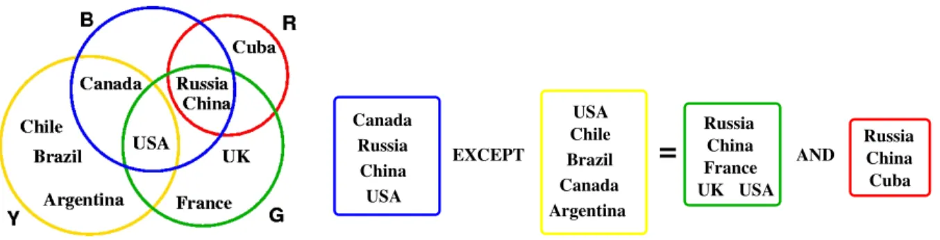
EXCEPT ANDFigure 1: (left) Example input to redescription mining. (right) Sample redescription. The expressionB−Y can be redescribed intoG∩R. 1/01/2004 1/02/2004 1/03/2004 1/04/2004 7/01/2004 7/02/2004 7/03/2004 7/04/2004
<35 F<50 F>60 F>75 FRainyCloudyWind > 5MPHDaylight > 10h
1/01/2004 1/02/2004 7/02/2004 7/03/2004 7/04/2004 7/01/2004 1/03/2004 1/04/2004
>75 F>60 FDaylight > 10hCloudyRainy<50 FWind > 5MPH
Figure 2:(left) Example input to biclustering. (right) Layout of computed biclusters.
2
Compositional Data Mining
Compositional data mining is not intended to be a one-size-fits-all data mining technique; rather, it is a way of problem decomposition based on the notions of biclusters and redescriptions. We begin by reviewing these primitives: whereas redescriptions relate object sets within a domain, biclusters relate object sets across domains.
2.1 Redescription Mining
As the term indicates, to redescribe something is to describe anew or to express the same concept in a different way. The input to redescription mining is a set of objects and a collection of subsets defined over this set. It is easiest to illustrate redescription mining using an everyday example. Consider the set of ten countries shown in Figure 1 and its four subsets, each of which denotes a meaningful grouping of countries according to some intensional definition. For instance, the colors (G) green, (R) red, (B) blue, and (Y) yellow (from right, counterclockwise) refer to the sets ‘permanent members of the UN security council,’ ‘countries with a history of communism,’ ‘countries with land area> 3,000,000square miles,’ and ‘popular tourist destinations in the Americas (North and South).’ We will refer to such sets asdescriptors. A redescription is a shift of vocabulary and the goal of redescription mining is to identify subsets that can be defined in at least two ways using the given descriptors. An example redescription for this dataset is ‘Countries with land area
>3,000,000square miles outside of the Americas’ are the same as ‘Permanent members of the UN security council who have a history of communism.’ This redescription defines the set{Russia, China}, first by a set
TFs
Phenotypes
Genes
Genes
TFs Genes Genes Phenotypes
Figure 3: Finding transcription factors (TFs) whose knock-down induces improved desiccation tolerance inC. ele-gans. (left) Two biclusters (shaded rectangles) joined at the gene interface using an (approximate) redescription. (right) Compositional data mining schema, displaying the sequence of primitives. Here, arrows indicate redescriptions, and dotted lines indicate biclusters.
Genes Genes
Orthologs
Worm Age Fly Age
GenesWorm GenesWorm GenesFly GenesFly Age
Worm
AgeFly
Figure 4: Finding shared gene expression programs in adult aging inC. elegansandD. melanogaster. (left) Three biclusters with redescription mining at the two gene interfaces. (right) Compositional data mining schema, displaying the sequence of primitives. As before, arrows indicate redescriptions, and dotted lines indicate biclusterings.
intersection of political indicators (G∩R), and second by a set difference involving geographical descriptors (B−Y). Notice that neither the set of objects to be redescribed nor the ways in which descriptor expressions should be constructed is input to the algorithm. The underlying premise of redescription analysis is that sets that can indeed be defined in (at least) two ways are likely to exhibit concerted behavior and are, hence, interesting.
2.2 Biclustering
The input to bicluster mining [32] is a set of instances of a relationship between two or more domains. Figure 2 describes relationships between dates (rows) and weather conditions (columns) in Blacksburg, VA. A bicluster is a subset of rows along with a subset of columns with the property that each row element is related to each column element (later we will utilize stricter notions of biclusters, but this definition will suffice for this example). Figure 2 (bottom) lays out the seven biclusters in the matrix as contiguous sub-matrices by re-ordering the rows and columns of the matrix [24], repeating rows and columns if necessary. For example, the bicluster spanning rows three through six and columns two through four states that each of the four days from July 1–4, 2004 experienced each of the weather conditions “>60 F,” “Daylight>10 h,” and “Cloudy.”
2.3 Composing Biclusters and Redescriptions
Both redescriptions and biclusters have direct applications in bioinformatics. Redescriptions are useful in relating gene sets from vocabularies based on cellular location (e.g., ‘genes localized in the mitochondrion’), transcriptional activity (e.g., ‘genes up-regulated two-fold or more in heat stress’), protein function (e.g., ‘genes encoding proteins that form the Immunoglobin complex’), or biological pathway involvement (e.g., ‘genes involved in glucose biosynthesis’). Similarly, biclusters are useful when we want to identify, e.g., sets of genes together with sets of experiments or sets of phenotypes that exhibit concerted co-occurrences. However, they have complementary advantages and limitations.
Redescriptions not only identify concerted sets but can also give meaningful characterizations of them in terms of data descriptors. This capability is akin to conceptual clustering [21, 35], where clusters are required to satisfy describability constraints. On the other hand, biclusters extensionally enumerate elements of subsets from both domains; we must do a post-analysis of the contents of these sets to describe them. Conversely, redescription mining requires that all descriptors be stated over a common universal set, so that data spanning multiple relations must be collapsed into one of the underlying domains. For instance, a relationship between genes and transcription factors might be used to define descriptors over genes. On the other hand, biclustering retains the relational nature of information and models patterns in relations. It is hence natural to combine their complementary capabilities.
To illustrate CDM, let us revisit the two scenarios from the introduction. The first scenario can be mod-eled by mining biclusters between genes and the transcription factors that regulate them, mining biclusters between genes and the phenotypes that result when they are knocked down, and connecting one side of the first bicluster to one side of the second bicluster using a redescription (see Figure 3). The second scenario can be modeled by mining three biclusters—for the relationship between worm genes and worm age, for the relationship between fly genes and fly age, and for the orthology relationship between fly genes and worm genes (see Figure 4). To cascade these three biclusters together, we can use two redescriptions as interme-diaries, one redescribing worm genes, and the other redescribing fly genes. We can think of such cascading as either the biclustering algorithm supplying descriptors to the redescription algorithm, or the redescription algorithm specifying the objects that must participate in the biclustering. The results of such compositions can be read sequentially from one end to the other, not unlike a story. For instance, for the first scenario above, we might find that ‘genes regulated by superoxide dismutase and catalase transcription factors, when knocked down, will result in cells with a phenotype of hypersensitivity to oxidative stress.’ In general, such compositions can induce a graph of arbitrary topology in the underlying data model, as we will see later.
Unlike the example in Figure 1, observe that both the CDM scenarios from Figs. 3 and 4 do not involve any constructive induction of descriptors in the redescriptions. There are situations where this feature is important, e.g., we may desire to find patterns such as “genes regulated by superoxide dismutase and catalase transcription factors but notby transcription factors that control the cell cycle, when knocked down, will result in cells with a phenotype of hypersensitivity to oxidative stress as well as abnormal cell size.” To mine such patterns, each redescription must potentially relate two or more biclusters on either side. In this first paper on CDM, we define descriptors as the “projections” of biclusters onto the relevant domains and focus on redescriptions with only one bicluster on each side, rather than on connecting set-theoretic combination of bicluster projections.
The Proteus vision of a CDM system is that a biologist can merely specify the domains that must partic-ipate in the composition (e.g., “TFs” and “phenotypes”) and the system automatically identifies a suitable composition of mining algorithms to relate the given domains. Observe that it can be infeasible to real-ize CDM by propositionalization, i.e., by first ‘multiplying’ out the original multi-relational dataset into a single-relation dataset, mining patterns in the integrated set, and then unpacking the pattern to relate the given domains. Although propositionalization has proved to be viable in traditional inductive logic pro-gramming [29], such algorithms only need to relate individualobjects across domains, whereas we must relatesetsacross domains, which are much larger in number and not defineda priori. In essence, CDM is relational knowledge discovery [20] over sets, instead of objects. It is also wasteful to organize indepen-dent redescription and biclustering results across the different domains and relationships, since many of the patterns mined would not participate in any connections.
Another approach to CDM might be to start by computing biclusters in one relationship and use them to constrain the mining [8] of biclusters in a neighboring relationship. However, such constraint-based
mining is ill-equipped to deal with the arbitrary expansion and contraction of descriptor sizes that CDM must support. Nevertheless, there are several significant structural properties of CDM patterns that we will exploit to design efficient mining algorithms.
The key contributions of this paper are as follows:
1. We formulate the notion of compositional data mining as an approach to better conceptualize struc-tured data mining problems. Rather than developing special purpose algorithms for every new type of dataset or analysis goal, CDM helps to organize knowledge discovery tasks in a modular manner. 2. Since CDM patterns connect sets of entities through alternating biclusters and redescriptions, we
present a new “compose then compute” algorithm that combines two biclustering and one redescrip-tion mining invocaredescrip-tions in a single step. This primitive significantly speeds up the composiredescrip-tion process and also avoids wasteful data mining.
3. Using the pattern mined by this integrated algorithm as a primitive, we show how mining composi-tional patterns reduces to systematic searches for joins over a suitably defined “CDM schema”. We can derive the CDM schema automatically from the original schema. Entities in the CDM schema representsetsof objects in the original schema. Recall that these sets are not defineda priori. They are mined by the compose then compute algorithm.
4. We leverage classical levelwise principles, in the spirit ofApriori[3] and WARMR [17], and extend them to find CDM patterns. This extension greatly broadens the applicability of the optimizations in these algorithms, just as the query flocks paradigm [53] generalized theApriori“trick” to general conjunctive queries.
3
Formalisms
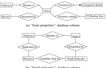
In this section, we introduce a sequence of formalisms beginning with database schemas, followed by data descriptors, redescriptions, and biclusters, culminating in CDM queries that will be of interest in this work. We use two running examples to illustrate these ideas. The first example relates four aspects of a gene’s function and regulation: the pathways it is a member of, the (unique) cytogenetic band it is contained in, the transcription factor (TF) binding sites present in its promoter, and stresses that up-regulate the gene. The second example relates small molecules to diseases they may treat and to genes they up-regulate, and pathways to diseases they are implicated in and genes that are their members. We will refer to these examples as “Gene properties” and “Small molecules”, respectively.
3.1 Database Schemas
Anentity setis a set of objects from a particular domain, e.g., genes, proteins, TF binding sites, or pathways. Objects in an entity setE can have values for a set ofproperties, denotedPE. Given two entity setsEand F, a(binary) relationshipR(E, F)betweenEandF is a subset ofE×F; we say thatRisconnectedto
EandF. It is useful to viewRboth as a binary matrix and as a bipartite graph. For example, relationships may connect proteins to each other via physical interactions, genes to TF binding sites in their promotors, or genes to pathways they belong to. In this paper, we consider only binary relationships although relationships of higher cardinality can be re-stated in terms of (multiple) binary relationships.
Given a setE of entity sets and a setR of relationships between entity sets inE, a database schema
Genes
Pathways Member of
Stresses Upregulated by Promoter contains TF Binding Sites
Cytogenetic Bands Contained in
(a) ”Gene properties”: database schema
Implicated in Upregulated by Member of Pathways Diseases Genes Small molecules Candidate drug for
(b) ”Small molecules”: database schema
Figure 5: Database schemas for two examples.
relationships) and whose edge set comprises edges each of which connects a relationship inRto an entity set inE. Observe that all nodes inRare constrained to have degree two inS whereas there are no degree constraints on the nodes inE. Figure 5 displays the schema for our two examples.
Although typical database schema specification languages such as SQL DDLs capture more information, we use the term database schemas in this paper to primarily refer to the graph structure of entities and relationships.
3.2 Descriptors and Redescriptions
Adescriptorover an entity setEidentifies a subset of entities fromE. The typical way to define a descriptor is as a boolean expression over a subset of properties Q ⊆ PE. For instance, the set of entities with a
particular value for an attribute, e.g., ‘the set of proteins with molecular weight equal to 100 kDa,’ is a descriptor. Relationships can also yield descriptors. For instance, using the relationship connecting genes to pathways they participate in, ‘genes in the Kit receptor pathway’ constitutes a descriptor over genes. To accommodate such descriptors, it is useful to think of the set of propertiesPE as being augmented from
attribute-value definitions to relational definitions. Henceforth, we will usePE to denote properties defined using both means. Given a descriptord, we will denote the set of entities for whichdis true byE(d).
Two descriptors d1 and d2 over an entity setE are said to be redescriptions of each other, denoted d1⇔d2, if they are distinct and approximately induce the same subset of entities fromE. The distinctness
condition rules out tautologies, e.g., an equivalence such asP1∩P2 ⇔ P1−(P1−P2)is not interesting
because it holds inalldatasets. The second condition can be evaluated by measures such as the support and Jaccard’s coefficient. The support of a redescriptiond⇔d0is given by the cardinality of the intersection of both descriptors, i.e.,|E(d) ∩ E(d0)|. The Jaccard’s coefficient ofd⇔d0 is given by ||EE((dd))∪∩EE((dd00))||. It is
zero if the descriptors are disjoint and one if they are the same. We will typically use the support constraint as a parameter to redescription mining and the Jaccard’s coefficient (and other measures) to evaluate a mined redescription. We do so because biologists find it more natural to input the number of, say, common genes, rather than the Jaccard’s coefficient.
or Jaccard’s coefficient level, which will be implicit in the context). Note that redescriptions are symmetric, i.e.,ρ(d, d0) ≡ ρ(d0, d). We will sometimes abuse notation and use the expressionρ(d, d0) to refer to the redescription itself.
3.3 Biclusters
LetR(E, F)be a relationship between entity setsEandF. Abicluster(E0, F0)onRis a setE0⊆Eand a setF0 ⊆F such thatE0×F0 ⊆R, i.e., every pair of entities inE0×F0belongs toR. Further, the bicluster
(E0, F0)isclosedif
(i) for every entitye∈E−E0, there is some entityf ∈F0such that(e, f)6∈R, and (ii) for every entityf ∈F −F0, there is some entitye∈E0such that(e, f)6∈R.
That is, adding an entity inE−E0orF−F0to the bicluster will violate the condition defining the bicluster. We say thatE0andF0areprojectionsof the bicluster ontoEandF, respectively. Observe that projections are a natural way to define descriptors overEand overF.
Similar to the redescription predicateρ, we define a predicateβ(d, d0)that is true if and only if descrip-torsdandd0 constitute the projections of a closed bicluster. Observe that there is no requirement thatd
andd0be defined over the same entity set. Moreover, unlike redescriptions, except in special cases,β(d, d0)
does not implyβ(d0, d). To avoid confusion, we will present the arguments forβin the same order as the re-lationship from which it was derived. We will also use the expressionβ(d, d0)to refer to the closed bicluster
(d, d0).
We will find it convenient to expand a bicluster into a closed one. Given a bicluster(E0, F0), itsclosure is any closed bicluster(E00, F00)such thatE0 ⊆E00andF0 ⊆F00. Note that unlike the notion of closures used in association rule mining [55], this definition allows multiple biclusters to be closures of a given bicluster. This aspect will become relevant when we present our algorithms for compositional data mining.
We note that ifRis a one-to-one relationship fromEtoF, then every bicluster onRcontains exactly one element fromEand one element fromFand the number of such biclusters is|R|. Furthermore, ifRis many-to-one fromEtoF, then each bicluster onRcontains exactly one element fromF and the number of these biclusters is at most|F|. For many-many relationships, biclusters correspond to bicliques in the bipartite graph representingR.
In general, relationships can themselves have properties. For instance, gene expression data is a rela-tionship between genes and samples, where each (gene, sample) pair is associated with an expression value. For such relationships, we will assume the existence of appropriate algorithms [32, 52] for biclustering numerical data (see Section 6.2 for an example).
As in the case of redescriptions, we will typically mine biclusters by imposing a minimum support constraint (which can be specified over either or both domains involved in the relationship).
3.4 CDM Schemas
Given a database schemaS(E,R), itsCDM schemaS∧(E∧,R∧)is another database schema whose entity sets and relationships have a one-to-one correspondence with the entity sets and relationships ofS with the following properties:
Co−members of Contained in Cytogenetic Bands
Gene sets PathwaysSets of
Stresses Sets of
upregulated byCommonly co−containPromoters TF binding site cassettes
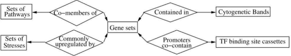
Figure 6: “Gene properties”: CDM schema.
(ii) Every relationshipR(E, F)inRis mapped to a relationshipR∧(E∧, F∧)inR∧ between the entity
setsE∧andF∧.
(iii) If(E0, F0) ∈ R∧(E∧, F∧), thenβ(E0, F0)is true inR,E0 is an entity inE∧, andF0 is an entity in
F∧.
Thus, an entity inS∧ maps to a set of entities inS. Figure 6 displays the CDM schema for the example in
Figure 5(a): the entity set “Genes” is mapped to “Gene sets”, the entity set “Stresses” is mapped to “Sets of stresses”, and so on. Similarly, the members of a pair belonging to the “Co-member” relationship inS∧
are the projections, onto the “Pathways” and “Genes” entity sets, of a closed bicluster on the “Member of” relationship. Since the relationship “Contained in” is many-one from “Genes” to “Cytogenetic bands”, the entity set “Cytogenetic bands” in the CDM schema represents single bands and not sets of them. Observe that redescriptions do not play a role in the CDM schema. (We will use them below in answering CDM queries.) Finally, the third condition in the formulation of the CDM schema implicitly enforces referential integrity constraints over the sets participating in all instances of relationships inS∧.
Lemma 1 IfR(E, F)is a relationship inE, thenR∧(E∧, F∧)is a one-to-one relationship.
Proof: Suppose thatR∧(E∧, F∧)is not a one-to-one relationship and that two pairs(E0, F0)and(E0, F00)
belong toR∧(E∧, F∧), whereE0 ∈E andF0, F00 ∈ F andF0 6=F00. By definition of the CDM schema, bothβ(E0, F0)andβ(E0, F00)are true inR. Thenβ(E0, F0∪F00)is also true, i.e., the bicluster formed by
E0andF0∪F00is also closed. SinceF06=F00, bothF0andF00are contained inF0∪F00, which violates the assumption that the original biclusters are closed. Therefore,R∧(E∧, F∧)is a one-to-one relationship. 2 Observe that Lemma 1 holds irrespective of the nature of the relationship inR.
There may not be a natural notion of a closed bicluster for relationships that have numeric attributes. In such cases, we will construct biclusters that ensure that Lemma 1 still holds.
With the construction of the CDM schema, observe that we are able to connectsetsof entities to each other via biclusters and redescriptions. The advantage of the above formulation is that a compositional mining query over the original schemaSnow reduces to a simple database join over the CDM schemaS∧. In particular, optimizations such as query flocks [53] can be readily applied to yield patterns that are actually comprised of sets of objects.
3.5 CDM Queries and Compositions
We now define the primary component of CDM queries and their results. A CDM query is a k-tuple
Genes
Pathways Member of
Stresses Upregulated by Promoter contains TF Binding Sites
Cytogenetic Bands Contained in
(a) ”Gene properties”: Database schema highlighting three entity sets in the sample query. Implicated in Upregulated by Member of Pathways Diseases Genes Small molecules Candidate drug for
(b) ”Small molecules”: database schema highlight-ing the two entity sets in the sample query.
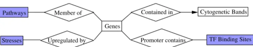
Figure 7: Two example CDM queries posed over database schemas.
illustrates two CDM queries, one for each of our examples. The first query specifies three entity sets: “Path-ways,” “Stresses,” and TF Binding Sites. The second query specifies the entity sets “Pathways” and “Small molecules.”
Informally, the semantics of the query is that the user is interested in compositions of biclusters and redescriptions involving the given entity sets, i.e., all the specified k entity sets must participate in the composition. Note that the user specifies the CDM query in the context of the original schemaS(E,R)and that this formulation only specifies the entity sets she desires to participate in the result. The user need not specify which relationships must participate in the query, or which other intermediate entity sets must be involved in the composition, since she may not know beforehand the intermediaries that will most usefully connect the entity sets of interest.
Observe that the user can obtain a trivial answer to such a CDM query by joining appropriate tables of the original schema. However, such answer will only yield compositions involving individual entities. As stated earlier, the crux of CDM is to compute compositions involving sets of entities.
The precise interpretation of the CDM query can refer to computing all compositions, testing for the existence of (at least) a composition, or counting the number of compositions. In this paper, we develop the CDM methodology in the context of computing all compositions. (Algorithms other than those proposed here might be more suited when we are trying to answer existence or counting queries.) We will also show how to impose constraints similar to the minimum support constraint popular in association rule mining.
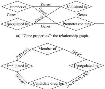
First, we define a transformation of the database schema S that we will use to translate CDM queries into composition plans. Therelationship graphΓ(S)of a database schemaSis a graph such that
1. nodes inΓ(S)have a one-to-one correspondence with the relationships ofS,
2. two nodes inΓ(S)are connected by an edge if the corresponding relationships share a common entity set inS. The edge is labeled by this common entity set.
Note that this concept is similar to the “relationship summary network” in [31] but captures the schema, instead of the instances. Informally, nodes in the relationship graph correspond to biclusters and edges
Promoter contains Contained in Member of Upregulated by Genes Genes Genes Genes Genes Genes
(a) “Gene properties”: the relationship graph.
Candidate drug for
Implicated in Upregulated by
Member of Genes
Pathways
Small molecules
Diseases
(b) “Small molecules”: the relationship graph.
Figure 8: Relationship graphs for the two illustrative CDM scenarios.
correspond to redescriptions over the entity sets labeling the edges. Figure 8 illustrates the relationship graphs for our two examples.
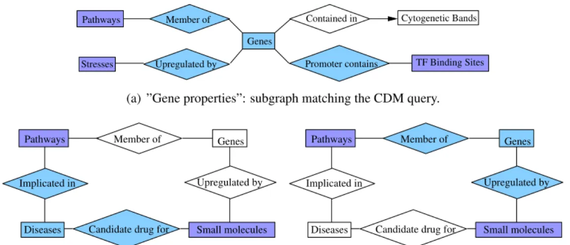
Given a CDM queryQ(E1, E2, . . . , Ek)on the schemaS(E,R), we say that a subgraphT ofSmatches QifT is connected andEi is a node ofT, for every1 ≤i≤ k. Such a subgraph “fleshes” out the query
by adding relationships and other entity sets in order to connect all the entity sets in the query. At this stage, we do not impose any constraints on the minimality of the subgraph that a query matches. Figure 9 displays the subgraphs matching the queries from Figure 7. Note thattwosubgraphs match the query for the “Small molecules” example. Moreover, the given schema for each of these examples is trivially a matching subgraph, which we do not display.
Now we define how to transform such a subgraph T into a subgraph ofΓ(S). Given a subgraphT of
Sthat matches a queryQ, therelationship graphΓ(T)ofT is the subgraph ofΓ(S)induced by the nodes that correspond to the relationships inT. We also say thatΓ(T)matchesthe queryQ. We observe without proof thatΓ(T)is unique and connected.
Next, we map relationship graphs matching a given CDM query to specific composition plans. Before we present the details of composition plans, it is helpful to have some additional definitions. We say that a closed biclusterβ(E0, F0)and a redescriptionρ(X, Y)composeifF0=X. We denote the composition by
βρ(E0, F0, Y). Another way in which closed biclusterβ(E0, F0)and redescriptionρ(X, Y)may compose is ifE0 =Y, denoted byρβ(X, E0, F0). Similarly, we can achieve a composition involving two biclusters by introducing a suitable redescription in between: the compositionβρβ(E0, F0, G0, H0)holds ifβ(E0, F0),
β(G0, H0), andρ(F0, G0) together hold. Observe that the two biclusters inβρβ(E0, F0, G0, H0) could po-tentially be derived from different relationships although the types ofF0 andG0 must be the same (for the redescription to hold). We use theβρβpredicates as building blocks for CDM.
Although not studied here in detail, we can also allow two redescriptions to compose directly. This capability and its extensions to more than two redescriptions has been previously studied [28].
Pathways Member of
Stresses Upregulated by
Contained in Cytogenetic Bands Genes
TF Binding Sites Promoter contains
(a) ”Gene properties”: subgraph matching the CDM query.
Upregulated by Member of Pathways Diseases Genes Small molecules Candidate drug for
Implicated in
(b) ”Small molecules”: the first subgraph matching the CDM query.
Pathways
Diseases
Genes
Small molecules Candidate drug for
Implicated in
Member of
Upregulated by
(c) ”Small molecules”: the second subgraph match-ing the CDM query.
Figure 9: Subgraphs matching CDM queries.
Genes
Genes
Genes Member of
Upregulated by Promoter contains
(a) ”Gene properties”: composition plan one for the matching subgraph.
Genes
Genes
Member of
Upregulated by Promoter contains
(b) ”Gene properties”: composition plan two for the matching subgraph.
Genes
Genes Member of
Upregulated by Promoter contains
(c) ”Gene properties”: composition plan three for the matching subgraph.
Genes Genes Member of
Upregulated by Promoter contains
(d) ”Gene properties”: composition plan four for the matching subgraph.
Figure 10: Composition plans for the CDM query in the “Gene properties” example.
Candidate drug for Implicated in
Diseases
(a) ”Small molecules”: compo-sition plan for the first subgraph matching the CDM query.
Upregulated by
Member of Genes
(b) ”Small molecules”: compo-sition plan for the second sub-graph matching the CDM query.
Γ(S)matching it,Φ(Q,T)is a set of bicluster predicatesβ ={β1, β2, . . . , βm}and a set of redescription
predicatesρ={ρ1, ρ2, . . . , ρn}such that
(i) there is a one-to-one correspondence between the bicluster predicates inβand the nodes inΓ(T). (ii) for every redescription inρthere is exactly one edge corresponding to it inΓ(T).
(iii) If a bicluster predicateβicorresponds to a node inΓ(T)and a redescription predicateρj corresponds
to an edge incident on that node, thenβiandρj compose.
(iv) the subgraph ofΓ(T)induced by nodes corresponding to bicluster predicates inβ and edges corre-sponding to redescription predicates inρis connected.
Note that an edge in this subgraph of Γ(T) and the two nodes incident on it correspond to a βρβ
pattern, reinforcing our decision to use these patterns as the building blocks of CDM. Just as there can be multiple subgraphs matching a CDM query, there can be multiple composition plans corresponding to a
(Q,Γ(T))pair. We can graphically depict any plan by highlighting the subgraph ofΓ(T)corresponding to plan (defined in condition (iv) above). For instance, Figure 10 displays four composition plans for the single subgraph that matches the CDM query for the “Gene properties” example and Figure 11 displays one composition plan each for the two subgraphs that match the CDM query for the “Small molecules” example.
4
Algorithms for CDM
To answer a CDM query, there are three key problems to be solved:
1. Identify all possible subgraphs of the given database schema that match the query. 2. For each subgraph, derive all specific composition plans.
3. For each composition plan, compute all relevantβρβpatterns.
We present efficient algorithms for each of these stages. For ease of understanding we present them in the reverse order, so that each algorithm feeds into the input of the next. Note that given an instance of a CDM schema and a composition planΦ(Q,T), finding satisfying assignments forβandρinΦ(Q,T)reduces to an database join overβρβpredicates.
4.1 ComputingβρβPatterns
At this stage, we are given two relationshipsR1(D, E)andR2(E, F)that share a common entity setEand
a support thresholdk > 0. Our goal is to compute satisfying assignments for theβ1ρβ2 pattern, whereβ1
(respectively,β2) is the bicluster predicate corresponding toR1 (respectively,R2) andρ is a redescription
predicate between descriptors over E such that the two descriptors participating in ρ contain at least k
elements in common.
4.1.1 Compute then Compose
In this section, we present a simple algorithm to compute the desiredβρβpatterns. This approach works by computing all biclusters inR1 and inR2 and computing redescriptions between all pairs of projections of
1. Compute the set of all biclusters inR1and inR2and their projections ontoE.
2. Insert these projections into a suitable index. Query the index with each projection to compute all its redescriptions.
3. For each redescriptionρ(X, Y)computed in the previous step, letB1(respectively,B2)
be the bicluster whose projection ontoE isX (respectively,Y). Store the βρβpattern corresponding to this triple.
4. Return all computedβρβpatterns.
For the purpose of this section, it is enough to assume that the indexing structure simply stores all projections. When given a query projectionP, it exhaustively computes all stored projections that contain at leastkelements in common withP.
4.1.2 Compose then Compute
A concern with the approach just described is that many computed biclusters will not participate in any redescription. In this section, we describe a technique that dramatically reduces the number of such orphan biclusters by mutually biclusteringR1 andR2.
Let D, E,andF be three entity sets inE and letR1(D, E)andR2(F, E) be two relationships, both
connected to the entity setE. Consider the relationshipR3(D∪F, E) =R1(D, E)∪RT2(F, E)formed by
taking the union of the pairs in the relationshipsR1(D, E)andR2T(F, E), where the pair(x, y)is a member
ofRT2(F, E)if and only if(y, x)is a member ofR2(E, F). We say that a bicluster(G, H)onR3(D∪F, E)
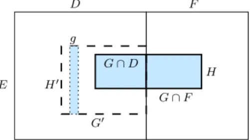
straddlesDandF ifGcontains at least one element fromDand at least one element fromF. We define thecomponentBA(G, H)ofB(G, H)inAto be the bicluster induced byG∩AandH onR(A, B). We define the componentBC(G, H)similarly onR(C, B). Note that the components themselves may not be closed. Figure 12 illustrates this situation.
H D F g G0 G∩D G∩F H0 E
Figure 12: An illustration of straddling biclusters. The two rectangles with thin borders represent the rela-tionshipsR1(D, E)andR2(F, E). The shaded rectangle with a solid thick border is the straddling bicluster
(G, H). The rectangle with a dashed thick border is a closure(G0, H0)of(G∩D, H). The dotted rectangle represents the elementg∈D.
Lemma 2 Let(G, H)be a closed bicluster onR3(D∪F, E)that straddlesDandF. Then the closure of
the bicluster(G∩D, H)onR1 is unique.
Proof: Let(G0, H0)be a closure of(G∩D, H). By definition of the closure, we have thatG0 ⊇G∩Dand
Assume to the contrary that there exists an elementg ∈ Dthat belongs to G0 −G∩D. Since(G0, H0)is a bicluster, for everyh∈H0, the pair(g, h)is a member of the relationshipR1(D, E). SinceH0 ⊇H, we
see that(G∪ {g}, H)is a bicluster onR3(D∪F, E), which contradicts the fact that the original bicluster
(G, H)is closed. Therefore,G0 =G∩D. Now consider an elemente∈ E such that for allg ∈ G∩D, the pair(g, e)is a member of the relationshipR1(D, E). By the definition of the closure,H0is the set of all
such elementse;H0containsHand is unique. 2
This lemma suggests that instead of computing biclusters separately inR1andR2and subsequently
search-ing for redescriptions between their projections ontoE, we can directly compute biclusters with at leastk
inR3and use the closures of its “components” inR1 andR2 as seeds for redescription computations. Our
modified algorithm to computeβρβpatterns has the following steps:
1. (a) Construct the relationshipR3(D∪F, E).
(b) Compute all straddling biclusters inR3with at leastkelements fromE.
(c) For every bicluster(G, H)computed in Step 1b, compute the closures of the biclus-ter(G∩D, H)onR1 and of the bicluster(G∩F, H)onR2.
(d) LetP1(respectively,P2)denote the set of projections ontoE of the closures
com-puted in Step 1c in relationshipR1(respectively,R2). Compute all closed biclusters
inR1 (respectively,R2)with the property that the projection ontoEof each such
bicluster contains at least one of the projections inP1(respectively,P2).
2. Identical to Step 2 of the compute then compose algorithm, but applied only to the biclus-ters computed in Step 1d.
3–4. Identical to Steps 3 and 4 of the compute then compose algorithm.
We now prove that the modified algorithm computes every redescription that the first algorithm does.
Lemma 3 Let(W, X)be a closed bicluster onR1and(Y, Z)be a closed bicluster onRT2 such thatW ∩Y
contains at leastkelements. Then the algorithm presented above computes the redescriptionρ(X, Y).
Proof: It is enough to show that the algorithm will compute the two biclusters either in Step 1c or in Step 1d. We will prove that the algorithm will compute(W, X). The proof for(Y, Z)is analogous. LetU =X∩Z. Assume that there exists a closed bicluster(S, T)onR3 such thatU ⊆T ⊆X. SinceT has at leastk
elements, the algorithm computes(S, T)in Step 1b. By Lemma 2, the closure of(S∩D, T)is unique. Let this closure be(S∩D, T0). We claim thatT0 ⊆X. Observe thatS∩Dmust containW. Therefore, ifT0
contains an elemente6∈X, sinceeshares a relation with every element ofS∩D,emust share a relationship with every element ofW, contradicting the fact that(W, X)is closed. Since the algorithm computes(S, T)
in Step 1b, it must compute(S∩D, T0)in Step 1c. In other wordsT0is an element of the set of projections
P1. SinceT0 ⊆X, we now see the algorithm computes(W, X)in Step 1d.
It remains to show that there exists a closed bicluster(S, T)onR3such thatU ⊆T ⊆X. Consider the
(possibly non-closed) bicluster(W, U)onR1. Consider the closure(W0, U0)of(W, U)such that|U0−U|
is the smallest over all such closures. Clearly,U0 ⊆X. Similarly, consider the bicluster(Y, U)onR2and
its closure(Y0, U00)onR2such that|U00−U|is the smallest over all such closures. Now,U00⊆Z. Setting S =W0∪Y0andT =U0∩U00yields us the required bicluster. 2
As we will show in Section 5, the improved algorithm significantly reduces the number of orphan biclusters while ensuring that we compute exactly the same number of redescriptions.
A final observation is that even for the two given relationshipsR1(D, E)andR2(E, F), there may be
multipleβρβpatterns possible. IfDandE are identical andR1 is not symmetric, then there are twoβρβ
patterns possible, depending on which “side” ofR1is used in the redescription withR2. An example is when R1 represents genetic interactions where the knock-out of one gene results in a phenotype that enhances or
suppresses the phenotype obtained by knocking out the other gene. For such relationships, we define twoβ
predicates for each bicluster, one being the transpose of the other. (Observe that, in addition, ifEandF are identical andR2is asymmetric, there are four possibleβρβpatterns.)
4.2 Levelwise Search for Compositional Patterns
We view the ‘compose then compute’ algorithm as an approach to find satisfying assignments for βρβ
predicates. Then the search for a compositional pattern reduces to relational data mining over the βρβ
relation. In the following, we will assume that at least two relationships are involved in a compositional pattern (mining one relationship is the task of traditional bicluster mining so that an expressive primitive such asβρβis not required).
In traditional relational mining algorithms such as WARMR [17], which support general Datalog queries, the search space of possible patterns is huge, so declarative language biases are imposed. Proteus, too, re-quires biases to curtail the complexity of search. Before we describe these, it is instructive to examine the structure of a sample composition plan.
Consider the threeβρβpredicates—β1ρ1β2,β2ρ1β3, andβ1ρ1β3—derived from four entity sets, three
of whom have binary relationships to the fourth (which supplies the redescription interface ρ1). Given a
CDM query that requires participation of all four entity sets, there are four composition plans possible (the ‘,’ denotes conjunction):
• β1ρ1β2(X, Y, Z, W),β1ρ1β3(X, Y, L, M). • β1ρ1β2(X, Y, Z, W),β2ρ1β3(W, Z, L, M). • β1ρ1β3(X, Y, L, M),β2ρ1β3(W, Z, L, M).
• β1ρ1β2(X, Y, Z, W),β2ρ1β3(W, Z, L, M),β1ρ1β3(X, Y, L, M).
(We use capital letters denote arguments; recall that they denote sets of objects from the respective domains). Observe the implicit reuse of arguments across predicates, so that the following composition is not legal:
• β1ρ1β2(X, Y, Z, W),β1ρ1β3(R, S, L, M).
The typical way in which illegal compositions are avoided is to adopt a canonical ordering for predicates in conjunctive plans and to usemodedeclarations that impose restrictions on how variables are introduced by the predicates. Thus, a mode of ‘-’ means that the variable can be bound by the predicate itself, ‘+’ means that it must be bound before the predicate is invoked, and ‘±’ means that it can either be bound before or by the predicate. To prevent the above illegal composition, we can specify the mode declarations for the
β1ρ1β2andβ1ρ1β3predicates as • β1ρ1β2(−,−,−,−) • β1ρ1β3(+,+,−,−)
which ensures that the first two arguments of β1ρ1β3 are bound earlier (in this case, by β1ρ1β2). Rather
than specify one global set of mode declarations for all compositional patterns, we exploit the fact that the bicluster predicatesβi in theβρβs are typed and that everyβρβ predicate can be used at most once in a composition plan (recall the definition in Section 3.5). With these constraints, it is easy to see that the modes should be ‘-’ for all arguments of the first predicate, and for every predicate following it, use ‘+’ for the mode if the bicluster corresponding to those arguments already participates in a previousβρβ, and ‘-’ otherwise.
Typical levelwise algorithms used in data mining use the notion of support to prune searches. However, defining a notion of support for CDM patterns is problematic. Due to the multiple shifts of vocabulary that happen in biclusters in a composition, there may be no single domain over which we can define support. It may be possible to define support in database schemas where there is a single domain participating in every relationship. In such a case, since every CDM pattern will involve that domain, we can measure support as the number of entities from that domain that participate in every bicluster in the composition.
A more general approach, used in algorithms such as WARMR [17], is to designate a subset of variables as thekey. The frequency of a pattern is then defined as the number of satisfying assignments to the key for which the pattern is true. This is a natural notion in WARMR whose predicate arguments are individual-based whereas the predicate arguments in Proteus are set-individual-based. A literal mapping of this definition to our relational setting would apply, for instance, if we are seeking ‘biclusters that participate in at leastk
compositions.’ However, the more natural interpretation for biologists is to find ‘compositions of biclusters and redescriptions that involve at leastk(key) objects.’ (In our applications, the key is typically a central biological object of interest such as genes, or proteins.) In other words, although we have elevated the representation language from objects to sets, data mining constraints are more naturally specified at the object level. Hence, this is the definition we adopt which also affords a levelwise algorithm. In particular, to find compositions of lengthmthat involve at leastkobjects, we search bottom-up, from level 1 to levelm−1
forβρβs andβρβcompositions that involve at leastkobjects. Due to the anti-monotonicity principle, if a sub-composition does not have support, we need not explore the lattice ofβρβpatterns that are a superset of the sub-composition. Observe that this allows to ‘push’ the support constraint into the algorithm for computingβρβs, as discussed in the previous section.
Two other considerations are those of logical redundancy of βρβcompositions and the specialization relation used to traverse theβρβ lattice. Since our compositions are non-recursive, no redundant compo-sitions should be introduced as long as we adopt a canonical ordering ofβρβpredicates, such as Rymon’s enumeration strategy [47]. However, a more subtle notion of redundancy arises if the original relationship run from an entity set to itself. Consider for instanceβ1derived from a genes-to-genes relationship based on
whether their protein products interact, andβ2derived from a genes-to-genes relationship based on whether
the protein product of one transcriptionally regulates the other. In this case, there are two ways in which the biclusters can be related by a redescription, depending on whether the protein interaction relationship extends the transcription regulators or the regulated genes. As mentioned in the previous section, this re-dundancy is handled at the level of computingβρβs itself, so that the notion of strong typing continues to hold when we compose theβρβs. The specialization relation is necessary in order to generate candidates. For instance, β1ρ1β2(X, Y, Z, W) can be specialized to eitherβ1ρ1β2(X, Y, Z, W), β1ρ1β3(X, Y, L, M)
or toβ1ρ1β2(X, X, Z, W)(the latter makes sense only for symmetric relationships). Again, sinceβρβs are
computed by the ‘compose then compute’ algorithm, we do not have to explicitly search for such assign-ments. These considerations lead to a straightforward implementation of a levelwise miner along the lines ofApriori[3] and WARMR [17], which we do not describe in detail in this paper.
4.3 Identifying Matching Subgraphs
Finally, given a CDM query, we address the problem of identifying the relationships and intermediate entity sets that must participate in the composition, which in turn influences the choice ofβρβs that can be used. The necessary condition here is that the subgraph induced over the database schema should be connected. This is necessary for theβρβs to be composable. (It is not sufficient, however, without proper mode dec-larations, as we saw in the previous section.) If we desire to minimize the number of new entity sets and relationships that are introduced, one possible formulation of this problem is as a computation of a Steiner tree over the database schema. However, cyclicity is not an undesirable feature in a CDM composition and we sometimes might prefer longer compositions, for ease of interpretation. In our current implementation, we exhaustively enumerate all possible subgraphs of the database schema, subject them to membership checks for the domains constrained by the CDM query and, from those that satisfy, identify all theβρβs that constitute the subgraph.
5
Effectiveness of CDM
Standalone algorithms for redescription mining and biclustering are already heavily tuned. Therefore, the effectiveness of CDM lies in its ability to avoid wasteful computations of biclusters and redescriptions that will not participate in any composition and, for theβρβpatterns that remain, being able to efficiently compose them in the levelwise miner. We have already shown how βρβ patterns serve as an important primitive for composition. Hence, in this section we address two questions of algorithmic effectiveness:
(i) What are the savings to computingβρβpatterns over separate biclustering and redescription invoca-tions?
(ii) How does the levelwise search for compositions scale with the length of the composition?
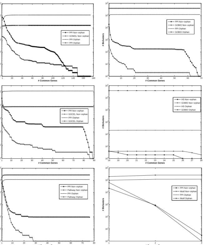
We address the first question by assessing, for various pairs of relationships that share a common domain, the number of biclusters that are “orphaned” on either side as a function of the support constraint of theβρβ
pattern. Figure 13 depicts these plots for variousβρβ predicates, using relations from a database schema that is described later in Section 6.2. (The exact details of these relations are not as important as the overall trends.) Each plot depicts four curves, two for each bicluster predicate; one curve tracks the number of non-orphan biclusters and the other the number of non-orphan biclusters, both as functions of the support threshold. Observe that, in general, differences between the number of orphans and the non-orphans can be as great as one to three orders of magnitude. For the plots on the left of Figure 13, for low support thresholds, the number of orphans is smaller than the number of computed biclusters but as the support threshold is increased (number of genes in common, in this case), we see greater numbers of biclusters getting orphaned. For the plots on the right of Figure 13, the number of orphans far exceeds the number of non-orphans, even for low support thresholds. These plots confirm that wasted computation of orphan biclusters is indeed a critical issue in CDM, and highlight the important role played by the compose then compute algorithm developed here.
We study the second question as a function of length of composition, i.e., the number of relationships participating in it. Thus, the simplest composition, involving twoβρβpredicates, has length3. Again, we use the case study described in Section 6.2 but this time consider the set of all βρβ patterns as a whole. We mineβρβ patterns at a lenient support constraint of 1. However, even though there is one entity set participating in almost all relationships, we do not impose any support constraints in the levelwise miner.
1 20 40 60 80 100 120 140 160 180 100 101 102 103 104 105 106 # Common Genes # Biclusters PPI Non−orphan GOMOL Non−orphan PPI Orphan PPI Orphan 1 10 20 30 40 50 60 70 100 101 102 103 104 105 106 # Common Genes # Biclusters PPI Non−orphan GOBIO Non−orphan PPI Orphan GOBIO Orphan 1 10 20 30 40 50 60 70 80 90 100 101 102 103 104 105 # Common Genes # Biclusters PPI Non−orphan GOCEL Non−orphan PPI Orphan GOCEL Orphan 18 19 20 21 22 23 24 25 26 27 28 100 101 102 103 104 105 106 # Common Genes # Biclusters HS Non−orphan GOBIO Non−orphan HS Orphan GOBIO Orphan 1 10 20 30 40 50 60 70 80 100 101 102 103 104 105 106 # Common Genes # Biclusters PPI Non−orphan Pathway Non−orphan PPI Orphan Pathway Orphan 1 2 3 100 101 102 103 104 105 106 # Common Genes # Biclusters PPI Non−orphan Motif Non−orphan PPI Orphan Motif Orphan
Figure 13: Assessing the number of “orphan” biclusters avoided as well as the actual biclusters computed (non-orphans) by the “compose then compute” algorithm. Each of the six plots involves a differentβρβ
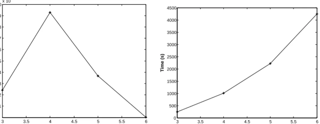
3 3.5 4 4.5 5 5.5 6 1 2 3 4 5 6 7 8 9 10x 10 6 Length of Chain # Chains 3 3.5 4 4.5 5 5.5 6 0 500 1000 1500 2000 2500 3000 3500 4000 4500 Length of Chain Time (s)
Figure 14: (left) Number of compositions mined as a function of the length of the composition. (right) Time taken to mine all compositions.
As a result, we may obtain compositions where one set of entities can gradually “morph” into another set of entities without any overlap. Thus, not imposing support constraints allows us to push the levelwise miner to its limits since it may be forced to evaluate a very large number of candidate compositions. Fig. 14 (left) displays the number of patterns mined as a function of composition length. Observe that there is initially an increase in number of patterns with length of composition but this number drops off steeply for higher values (there are no patterns mined of composition length7or more). It is significant that, for a schema with
9relationships, we find compositions of length6(although not quite evident in Figure 14 (left), there are45
of them). This statistic demonstrates that there are significant opportunities for CDM in real multi-relational datasets. The output-sensitive nature of the levelwise algorithm is evident in Fig. 14 (right) which tracks the time taken to mine compositions as a function of composition length. (Recall that due to the lax support constraint, the algorithm would be evaluating an exorbitant number of candidates.)
6
Case Studies
Our first case study (GO3) mines overlaps in functional annotations across all three categories of the Gene Ontology (GO) using human (H. sapiens) genes as the underlying universal set. The results of this study help understand implicit dependencies between terms from different GO categories and potentially to use these dependencies to predict new gene-term associations (an aspect beyond the scope of the present paper). The second case study (‘Stress Response in Human Cells’) focuses on understanding the molecular mechanisms of responses of human cells when they are subjected to different types of environmental stresses. Besides human genes and their membership in GO taxonomies, for this study, we also incorporate data about gene expression measured by microarrays, transcriptional motifs in upstream regions of genes, locations of genes in cytogenetic bands, protein-protein interactions, and pathway membership. Figures 15 and 20 display the schemas for these case studies. In both figures, dashed lines connect pairs of relationships between whose biclusters we compute redescriptions. Table 1 gives important statistics for both case studies. We provide one table since the data for the second case study subsumes the first.
Biological Processes Member of Genes Cellular Components
Performs
Molecular Functions
Localized to
Figure 15: The schema for the first case study involving GO functional annotations for human genes.
6.1 GO3
The Gene Ontology [4] is a controlled vocabulary to describe genes and their products across a range of organisms. The three categories of GO—biological process, molecular function, and cellular component— address diverse aspects of gene activity. Briefly, they address the “when,” “‘what,” and “where” of a gene’s activity in cells. Each category is organized as a directed acyclic graph (DAG) defined by parent-child relations between terms.
The dependencies we seek to mine are pairs of GO terms, each belonging to a different category, that are annotated by a surprisingly large number of common genes. In this study, each GO term yields exactly one bicluster consisting of that GO term and all the genes annotated with it. Some dependencies are obvious. For instance, we anticipate that the GO biological process ‘protein ubiquination’, the GO molecular function ‘ubiquitin ligase activity,’ and the GO cellular component ‘ubiquitin ligase complex’ should annotate nearly the same set of genes. Other such associations might be less obvious, however, and our goal is to mine them. Since terms in GO are specified at multiple levels of detail, it is not sufficient to evaluate dependencies simply based on the number of genes simultaneously annotating two functions. We use the following strat-egy, modified from Grossman et al. [23]. Given a terms, letnsbe the number of genes annotating the term. Given two termssandt, let ns,tbe the number of genes annotating both terms andn+s,tbe the number of genes annotating at least one parent of eithersort. We want to assess the surprise in observing thatsand
tannotatens,tgenes in common, conditioned on the fact that their parents annotaten+s,tgenes in total. We ask the following question: if we were to picknt genes uniformly at random without replacement from a pool ofn+s,t genes, what is the probability that we will selectns,t or more genes from a set ofns marked
genes? We take recourse to the familiar hypergeometric distribution to assess this probability, denotedps,t:
ps,t = Pmin(n + s,t,ns) k=ns,t ns k n+s,t−ns nt−k n+s,t nt .
Since we test the significance of multiple pairs of functions, we adjust thep-values using the false discovery rate [9]. Figure 16 depicts the steep drop in the number of redescriptions that meet increasingly stringent thresholds on either the Jaccard’s coefficient or the p-value. We plot separate curves for each pair of GO categories. Observe that the number of redescriptions between GO molecular functions and GO biological processes dominate the number of redescriptions between the other two pairs of categories. This trend reflects the fact that the number of cellular component terms is much smaller than the number of terms in the other two categories (see Table 1).
0.1 0.2 0.3 0.4 0.5 0.6 0.7 0.8 0.9 1 0 1000 2000 3000 4000 5000 6000 7000 8000 9000 10000 Jaccard’s Coefficient # Redescriptions Cel−Mol Cel−Bio Mol−Bio 10−300 10−200 10−100 100 0 500 1000 1500 2000 2500 3000 p−value # Redescriptions Cel−Mol Cel−Bio Mol−Bio
Figure 16: GO3 case study: distribution of the number of redescriptions. (left) Number of redescriptions that satisfy different Jaccard’s coefficient thresholds. (right) Number of redescriptions that meet different
p-value cutoffs. 50 100 150 200 250 300 350 400 450 500 0.1 0.2 0.3 0.4 0.5 0.6 0.7 0.8 0.9 1 #Connected components Jaccard’s coefficient 0 0.1 0.2 0.3 0.4 0.5 0.6 0.7 0.8 0.9 1 0.1 0.2 0.3 0.4 0.5 0.6 0.7 0.8 0.9 1
Relative size of largest connected component
Jaccard’s coefficient 0 1000 2000 3000 4000 5000 6000 7000 8000 0.1 0.2 0.3 0.4 0.5 0.6 0.7 0.8 0.9 1 #Triangles Jaccard’s coefficient
Figure 17: GO3 case study: distribution of the number of connected components (left), the relative size of the largest connected component (center), and the number of triangles (right) as a function of Jaccard’s coefficient.
significant at the0.01level. By construction, this graph is tripartite. We considered two types of patterns in this graph: triangles and non-triangles. A triangle connects three terms, one from each GO category, such that each pair has significantly overlapping sets of annotated genes. After removing all triangles from this graph, we study the remaining edges that comprise non-triangles. Figure 17 displays global statistics of the structure of this graph as we vary the Jaccard’s coefficient. Very few redescriptions satisfy a large Jaccard’s coefficient threshold. Therefore, the number of connected components in the graph is small, as is the relative size of the largest component in it and the number of triangles. As we decrease the threshold, more disconnected components start appearing. At a threshold of0.3, a giant component emerges. As the threshold decreases further, connected components start coalescing. Therefore, the number of connected components decreases. The other two curves are monotonic increasing with decreasing threshold, but show a sharp uptick at0.3, the point where the giant component forms.
The triangle and non-triangle patterns yielded numerous interesting insights, of which we highlight a few here. In the images we display, each node represents a term in GO (blue nodes are cellular components,
green nodes are biological processes, and magenta nodes are molecular functions).
(a) (b)
Figure 18: Examples of triangles in the GO3study.
Triangles Many triangles represented biological processes fundamental to the function of a cell such as
mitosis and important structural components such as the cell membrane. Processes such as mitosis have been studied at depth by biologists. Hence, it is not surprising that the cellular localization of the gene products driving these processes and the molecular functions have been worked out. We hypothesize that a number of annotations for human genes in such triangles are actually electronically transferred from lower organisms such asS. cerevisiae. Figure 18(a) displays a subgraph of connected triangles that relate to the process of spindle localization, a key component of cell division. The kinetochore is a protein complex located in the pericentric region of DNA . It provides a point where the microtubules of the spindles can attach. The aster is an array of microtubules that emanate from a spindle pole but do not attach to kinetochores. This subgraph suggests that asters and kinetochores together coordinate the localization of the spindle during cell division. Figure 18(b) displays a network of connected triangles “rooted” at the molecular function “GPI anchor transamidase activity”. GPI anchors attach membrane proteins to the cell’s lipid bilayer. This subgraph highlights other relevant processes and components involved in this function, e.g., the synthesis of phosphoinositides and the GPI anchor transamidase complex.
Non-triangles We observed that almost all pairs of terms connected by non-triangle edges related to
com-ponents, functions, and processes were unique to multi-cellular and higher order organisms. This observa-tion suggests that such concepts have not been experimentally well-studied in all three categories of GO. Laminins are glycoproteins that are major constituents of the basement membrane of cells. Figure 19(a) demonstrates that the function of binding with laminins is intimately linked to a very large and diverse set of processes: the development of the prostate and salivary glands, regulation of proteolysis, and cell fate spec-ification (the process involved in the specspec-ification of the identity of a cell), to name just a few. Figure 19(b) relates the cell soma, which is the portion of the cell bearing surface projections, to yet another large and diverse set of processes. These processes include stem cell division, regulation of heart contraction, the maturation of hair follicles, and biosynthesis of dopamine.
(a) (b)
Figure 19: Examples of non-triangles in the GO3study.
Genes MSigDB Motifs MSigDB Pathways GO Cellular Components GO Biological Processes GO Molecular Functions Time points Belongs to Gene Expression Localized to PPIs MSigDB Cytogenetic Bands Stresses Belong to Contains Member of Member of Performs
Figure 20: The schema for the second case study involving human PPIs, stress gene expression data, and MSigDB and GO functional annotations.
Name #Genes #Participants Domain type #Relationships Density
PPIs 9318 9318 Genes 45277 0.0005
Gene expression 13877 188 Timepoints 2420842 0.9279
Member of 15498 3307 GO Biological processes 301671 0.0059
Localized to 15498 657 GO Cellular components 171226 0.0168
Performs 15498 2618 GO Molecular functions 152246 0.0038
Member of 13197 1686 MSigDB pathways 106367 0.0048
Contains 9859 837 MSigDB Motifs 101523 0.0123
Belong to 29856 383 MSigDB Cytogenetic bands 60013 0.0052
Table 1: Statistics for the two case studies. We only display statistics for relationships involving genes. The first column states the name of the relationship. The second column lists the number of distinct genes participating in the relationship. The third column lists the number of participants from that relationship, whose type is given in the fourth column. The fifth and sixth columns state the number of pairs and density of the relationship. The database contains gene expression measurements for 13 different stresses, each comprising multiple time-points.
6.2 Stress Response in Human Cells
Our goal in this case study is to use CDM to understand the cellular contexts in which genes regulated by external stresses operate. We gathered a diverse set of data types to address this question. First, we obtained gene expression data characterizing responses of HeLa cells and primary human lung fibroblasts to heat shock, endoplasmic reticulum stress, oxidative stress, and crowding [38]. The dataset we analysed includes transcriptional measurements obtained by Whitfield et al. [54] for studying cell cycle arrest by using a double thymidine block or with a thymidine-nocodazole block. Overall, the gene expression data involves 13 distinct stresses over the two cell types. Next, we obtained a network of31108molecular interactions between9243human gene products by integrating the interactions in the IDSERVE database [45], the results of large scale yeast two-hybrid experiments [46, 49], and20immune and cancer signalling pathways in the Netpath database (http://www.netpath.org). The IDSERVE database includes human curated interactions from BIND [6], HPRD [42], and Reactome [27], interactions predicted based on co-citations in article abstracts, and interactions that transferred from lower eukaryotes based on sequence similarity [30]. Finally, we derived information about cytogenetic bands, transcriptional motifs, and pathway membership from MSigDB [50] and functional annotations for the genes in our network from the Gene Ontology (GO) [5]. Figure 20 displays the database schema underlying this data and Table 1 summarizes important statistics about this data.
Due to the multitude of data types available, we used a variety of algorithms for computing biclusters. We adapted a home-grown closed itemset mining algorithm to compute straddling biclusters. We used SAMBA [51] to discover biclusters in gene expression data. Since the human PPI network is quite sparse, we found that biclusters in the “PPIs” relationship to be very small in size. Therefore, we simulated the process of redescribing genes in SAMBA biclusters into genes in PPI biclusters by implementing an expansion operator: for each SAMBA bicluster, we constructed a PPI sub-network that included all genes in that bicluster with known PPIs. We connected pairs of these genes either directly (if they were interacting) or indirectly (if they had a common neighbor). Note that such PPI sub-networks may not be connected. The results we have presented in Section 5 use these biclustering algorithms and expansion operations to showcase the scalability of our CDM implementation for this case study.
A number of compositions we compute illustrate known themes about the cell’s response to stress. For instance, it is well known that when targeted by a stress, the cell shuts down the cell cycle in order to cope with the stress. Consistent with this observation, we find that compositions containing SAMBA biclusters with down-regulated genes also involve MSigDB pathways and GO biological processes related to various stages of the cell cycle. In addition SAMBA biclusters with up-regulated genes often compose with MSigDB pathways containing cell cycle regulators.
We highlight a CDM pattern that spans the “Gene Expression”, “PPIs”, “Member of” (MSigDB ways), and “Belongs to” (Stresses) relationships, thus connecting four entity sets. The two MSigDB path-ways in this pattern are “CMV HCMV TIMECOURSE ALL UP” and “GALINDO ACT UP”; we dis-cuss them in more detail below. This composition involves the response of fibroblasts to treatment with 2.5 mM dithiothreitol (DTT), which is known to induce endoplasmic reticulum stress. The SAMBA bi-cluster contains six time points (other than the “zero” point), all measuring the response to this stress. All genes in the bicluster are up-regulated, as displayed in Figure 21. The figure also displays the PPI sub-network corresponding to this bicluster. Here, a light green rectangle is a gene present both in the SAMBA bicluster and the PPI network; a light green ellipse is a gene present in addition in the MSigDB pathways that form this pattern; a white node is one that is introduced by the expansion operator. The “CMV HCMV TIMECOURSE ALL UP” pathway is a set of 470 genes up-regulated in fibroblasts follow-ing infection with human cytomegalovirus [11]. The presence of this pathway in this pattern suggests that the endoplasmic reticulum may be targeted by the virus during infection. We find evidence in the literature supporting this CDM pattern. Ogawa-Goto et al. [39] found that p180, an integral endoplasmic reticulum membrane protein, interacts with a viral protein and that this interaction may play a role in the intracellular transport of the virus. “GALINDO ACT UP” is a set of 88 genes significantly up-regulated by the toxin Act in macrophages [22]. This CDM pattern suggests that the inflammatory response induced by this toxin may include stress to the endoplasmic reticulum.
Figure 21: Stress response in human cells: a CDM pattern that sheds light on fibroblast response to endo-plasmic reticulum stress. This pattern involves four relationships: “Gene Expression” (left), “PPIs” (right), “Member of” MSigDB pathways (not shown), and “Belongs to” stresses (not shown). See text for more details.
Another pattern spans the same relationships and entity sets. It highlights the response of HeLa cells to oxidative stress induced by administering hydrogen peroxide. As displayed in Figure 22, the genes in the SAMBA bicluster in this composition are heavily down-regulated in response to this treatment. The