EXAMINATION OF PHENOMENA AFFECTING THE DEPRECIATION OF FIXED ASSETS

(1)

CORVINUS UNIVERSITY OF BUDAPEST

EXAMINATION OF PHENOMENA AFFECTING THE

DEPRECIATION OF FIXED ASSETS

PhD Dissertation

Nándor Kaliczka

Budapest

2013

(2)

Nándor Kaliczka

(3)

Department of Managerial Accounting

Supervisors: János Bosnyák Ph.D

Rezs

ő

Baricz CSc

Copyright © Nándor Kaliczka, 2013.

All rights reserved.

(4)

Management and Business Administration PhD Programme

Examination of Phenomena Affecting the Depreciation of Fixed Assets

(PhD Dissertation)

Nándor Kaliczka

Budapest 2013

(5)

List of Graphs

Graph 1: Different dimensions and concepts of capital. (Source: own elaboration) ... 14 Graph 2: Relationship between the asset values as estimated and calculated using the

linear allocation method. (Source: own elaboration) ... 23 Graph 3: How the choice of linear allocation or the ‘change in the value’ method to

compute depreciation impacts on income. (Source: own elaboration) ... 24 Graph 4: Relationship between services embodied in the assets and periodical capital

stock. (Source: own elaboration) ... 44 Graph 5: The different asset efficiency patterns as a function of asset age. (Source: own

elaboration) ... 52 Graph 6: Age-value profiles eventuated by the different efficiency patterns. (Source:

own elaboration) ... 55 Graph 7: Evolution of service values without and adjusted for disembodied obsolescence throughout the individual periods. (Source: own elaboration) ... 58 Graph 8: Evolution of asset values without and adjusted for disembodied obsolescence

throughout the individual periods. (Source: own elaboration) ... 59 Graph 9: Evolution of service values without and adjusted for embodied obsolescence

throughout the individual periods. (Source: own elaboration) ... 61 Graph 10: Evolution of asset values without and adjusted for embodied obsolescence

throughout the individual periods. (Source: own elaboration) ... 62 Graph 11: Breakdown of the change in asset values according to age and time factors.

(Source: based on Hulten and Wykoff [1981a]) ... 66 Graph 12: Cross-section depreciation, time series depreciation and revaluation. (Source:

own elaboration) ... 67 Graph 13: Summary of the phenomena affecting the time series depreciation rate.

(Source: own elaboration) ... 73 Graph 14: Change in the asset value without certainty and exact knowledge about the

future (Source: own elaboration) ... 79 Graph 15: Prices of diesel-powered cars plotted against age and mileage. (Source: own

(8)

7

List of Tables

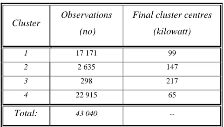
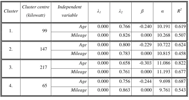
Table 1: Number of observation units in the individual clusters and the individual cluster centres. (Source: own elaboration) ... 95 Table 2: Estimated parameters of the Box-Cox transformation. (Source: own

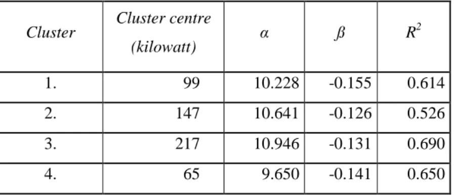
elaboration) ... 100 Table 3: Values of the regression based on the variable ‘age’. (Source: own elaboration)

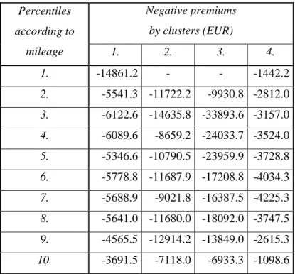
... 102 Table 4: Negative premiums in the individual clusters, broken down by clusters.

(Source: own elaboration) ... 103 Table 5: Depreciation rates computed for the individual clusters. (Source: own

(9)

8

1 Introduction

The concept of depreciation and the measurement of its value have long been a prominent issue in economic and accounting literature, the relevance of which is demonstrated by the great number of open questions related to the subject. In the last two centuries, several authors (researchers) dealt with the problem of depreciation, which not only contributed to the evolution of depreciation theory, but also gave rise to many new issues. The majority of these newly encountered problems appear to be inextricable, placing the subject in what seems to be an endless horizon.

The concept of depreciation is virtually inseparable from the concepts of capital and income, which appeared as individual measures in the economics literature of the early 20th century. It was not until the 1930s that economists began to focus on the interpretation of the concepts of business capital and income. One of the key issues in the determination of capital and income is how to measure the contribution of fixed assets to the corporate operational processes. The primary attribute of these fixed assets is that their service lifetime spans over several reporting periods. Preinreich [1937] differentiates between two main categories of fixed assets on the basis of the services these assets provide. One category encompasses assets providing a limited quantity of services, the other category includes fixed assets that have only limited possibilities to provide services.1 However, different approaches are needed to understand the consumption of the two categories of fixed assets; consequently in my dissertation I will only analyse the consumption of assets serving the company’s activity during several periods, created by man, with a finite service lifetime, and with quantitative limitations concerning usability (finite number of times of usage).2 Asset value consumption may be substantiated in the form of cost allocation, sinking funds or actual changes in value; however of the three, only the ‘actual change in value’ approach is appropriate to arrive at the correct asset and income values.

1_{Examples of this category include patents, brand names, trademarks, licenses among other, as well as}

elements of knowledge capital.

2

(10)

9

Depreciation captures a certain part of the changes in the values of fixed assets within a period;3 the manner of presenting this concept impacts business income as well as pricing the company’s output which needs to include costs related to the consumption of fixed assets, in addition to current costs. Therefore the choice of the method to capture depreciation also influences the company’s competitiveness on the capital and commodity markets. As a result, income calculation if faced with the problem of end-of-period valuation of fixed assets used (possessed), which is further complicated by the constant changes in prices.

The end-of-period value of fixed assets used may be calculated using the market prices of these assets or on the basis of the discounted present value of their future returns, where the return of the asset is usually identified as its theoretical rental. However, end-of-period valuation of assets in both methods is derived from market prices, which is problematic because in reality relevant markets for fixed assets hardly ever exist. As a consequence, the end-of-period asset value is determined using estimated depreciation rates calculated with due regard to the phenomena influencing asset value. In my dissertation, when attempting to determine depreciation, I shall mainly focus on the phenomena of exhaustion, deterioration and obsolescence, and analyse the effects of these using Jorgenson’s capital vintage model.

I will perform empirical tests based on supply-side information on the used car market using Box-Cox transformation, showing that passenger cars’ depreciation follows a geometric sequence pattern, where age has a stronger explanatory power than mileage. This may be attributed to the fact that obsolescence is asserted in the age variable, as confirmed by the results of the hedonic method and the paired t-test. The results of the empirical tests may also be useful for the determination and application of depreciation rates.

3

(11)

10

2 Income as the measure of economic performance

In economic and accounting literature, income means excess capital generated during a period and available for consumption, always determined from the point of view of a person or a group. However, the way of assigning such excess capital to a person or a group influences the content and the interpretation of the concept of income.

According to Lee [1986], the science of economics considers income as an individual measure; the founder of this personal income theory was Irving Fisher, who identified income as the monetary value of the enjoyment resulting from the consumption of goods and services. His definition does not consider any unconsumed capital increase (i.e. savings) to be part of the income, as he identifies saving as a kind of potential consumption, only resulting in satisfaction when actually consumed (Lee [1986]). However, later economists determined the income of a period t as the sum of consumption and saving , the saving being conceived as the variation of the individual economic capital within the period; i.e. = − . On the basis of the above, individual economic income may be expressed as

(1) = + − ,

where and means the end-of-period and beginning-of-period capital, respectively (Bélyácz [2002]).

The development of income theory in general is attributed to Hicks, who described his concept of income as follows:

“it would seem we ought to define a man's income as the maximum value which he can consume during a week and still expect to be as well off at the end of the week as he was at the beginning” (Hicks [1978] p. 207).

In the present case, the expression “well off” in Hicks’s definition may be identified with wealth or capital, the maintenance of which in its initial state is at the heart of Hicks’s income theory. However, several possible approaches exist in relation to the maintenance of capital intact, which I shall analyse in detail hereinafter.

(12)

11

The economic income concept presented above is also suitable for the measurement of corporate economic performance. Business income expresses the income of the owners of the company resulting from the given enterprise. As owners constitute a group which is homogeneous in respect of the company, the owners’ income (i.e. the company’s income) may be determined in analogy with individual income (Lee [1986]):

(2) = + − .

Business income is composed of the dividend paid or payable to the owners and of the changes in the business capital over the period − ; this change shall not include the effects of any eventual capital investment or disinvestment effectuated during that period. Dividend may be construed as the consumption of business capital by the owners, which once paid does not serve the operation of the company’s value creating processes any longer, and consequently may be entirely correlated with consumption determined in relation to economic income .

Equation (1) and (2) show that the value of the income is principally a function of the difference between the beginning-of-period and end-of-period capital. For an in-depth analysis of this value, in the following chapters I shall give a brief overview of capital-related theories as well as of their evolution.

2.1 A brief overview of capital theory and its evolution

The conceptual definition of capital is virtually a permanent issue in economic literature, with two principal approaches. Some of the authors define capital starting from its physical quantity, while others use its value as a starting point – it may thus be stated that capital possesses both a quantitative and a value-related dimension. Capital, in its value dimension, made an appearance as early as in classical economics, where land and work were considered to be the primary factors of production, and as a consequence, capital was regarded as the primary representative of work product (Bélyácz [1992]). Since the first half of the last century, capital theory has undergone substantive development due, among others, to Fisher. Fisher [1896] accepted the dominant view of the era considering that capital is constituted of a determined set of wealth categories, so any form of capital needs to include these accepted categories of wealth; this may actually be considered as the materialistic approach to capital value. Fisher criticised

(13)

12

Adam Smith’s thesis according to which a category of wealth may be considered as capital if it is capable to produce a revenue. According to Smith, a merchant ship is capital, whereas a private yacht is not, as it is only suitable for the satisfaction of its owner’s individual needs, and thus unable to produce revenue. However Fisher disputed this limitation of the capital concept: he considered that it is possible to identify deriving revenues for every kind of wealth, and through this line of argument he questioned the necessity of breaking down wealth into capital and non-capital elements (Fisher [1896]).

One of the debates on capital in early economic literature concerned the issue of differentiating between capital and income. Following Cannan, Fisher differentiated between capital and income on a time-related basis. In Fisher’s opinion, any wealth may be considered in respect of its relationship with time in one of two ways: either as “stocks of wealth” or as “flows of wealth”, the inseparability and interrelatedness of which was recognised with the general acceptance of capital value based on future returns. Fisher considers Cannan to be the first to lay the foundations of this relationship between capital and income, as he appears to be the first to have enunciated the precise time relation between these two concepts. According to Fisher [1896], Cannan stated that the wealth of an individual may mean two different things: either his possessions at a given point of time or his receipts for a given length of time. Like Marshall, Cannan conceived of income as a flow of pleasure, but of capital as a stock of things (Fisher [1896]).

Veblen also recognised the sameness of capital value and of the present value of the resulting future benefits (Bélyácz [1992]): he considered that the value of capital is determined by its expected ability to generate benefits. Thus, it has become possible to assess capital as a benefit generation unit, without a need to materialise it. Consequently, we may consider as capital wealth anything that is liable to produce economic benefit in future. With this extension, the concept of capital is no longer limited to tangible assets, which allows for factors identified as elements of the intellectual capital to be considered as part of the capital.4 As a result, in case of a capital stock with a complex structure, a vast part of the capital value is constituted by intellectual capital elements, seemingly “invisible” in the material sense, the existence of which is rather difficult to ex ante prove or disprove; and the number of these invisible elements continually grows

4

(14)

13

in parallel with the increasing complexity of capital in the material sense. As a consequence in case of a higher capital complexity, as far as structuration theory is concerned, Veblen’s capital value concept may only be concerted with Fisher’s materialistic capital concept (considering the individual wealth elements as representatives of the capital value in their physical quality) with a high level of uncertainty. The reconciliation of the two capital value concepts is further complicated by the fact that the above mentioned “invisible”, intellectual or human capital elements may only be identified in a subjective way, with a high level of uncertainty. Many tentatives have been (and are currently) made to dissolve the tension between the approaches to capital value as material unit on the one hand and benefit generating unit on the other hand; a common feature of these is that the differences between capital considered as a benefit generating or as a materialised unit are associated with elements which are difficult to observe in the present, such as “employee value” or “client value”, definable as wealth only from the benefit generating unit viewpoint, but not in the material sense. These conceptual differences constitute a long disputed issue in accounting theory; as a first step in their reconciliation, after a long process of pondering, certain “invisible” wealth elements, such as business value or corporate value, or the activated value of R&D, have finally been incorporated in the category of wealth elements recognised in accounting, which decreased the difference between the two basic approaches to capital outlined above.

A common feature in the two different capital concepts described hereinabove is that both aim to determine the value dimension of capital. However, an alternative approach to capital exists in economic literature, which examines capital from the point of view of its physical quantity, concentrating on its quantitative dimension, where the concept of capital is supposed to mean the totality of the (physically) productive physical services rendered by the wealth constituting the capital. The quantitative dimension of capital is mainly examined by the branch of economics researching into production theory. In the production theory framework, the physical unit of capital is more important than its value, for production theory revolves around the production function, representing the relationship between the quantities of the output on the one hand, and of the various inputs on the other hand (Griliches [1963]). For the physical dimension of capital, capital goods (or assets) are considered as a pool of potential future (physical) services to be utilised in the value creation processes. Actually, this approach is closely related to

(15)

14

the “benefit generating unit” concept of capital, as both consider capital to be a pool of potential future services. However in the case of the physical dimension, the analysed factor is the physical unit of the services, whereas in the case of the benefit generating unit concept, it is the value of the services.

The following chart illustrates the relationship between the two currently accepted capital dimensions described above and between their different concepts.

Graph 1: Different dimensions and concepts of capital. (Source: own elaboration)

The issue of measuring and grasping business capital also appears in the practice of business income calculation, the rules pertaining to which are usually set out in the financial reporting standards relevant to the given field. The International Financial Reporting Standards (IFRS) Framework differentiates between the physical and financial dimensions of capital. According to the Framework, the financial dimension of capital is measured in terms of invested money or invested purchasing power, capital being synonymous with the net assets or equity of the entity; whereas the physical dimension of capital regards capital as the productive capacity of the entity. This differentiation between capital dimensions corresponds with the capital dimensions described in the economic literature on capital, on the evolution and present state of which I have hereinabove elaborated.

Many theoretical debates concerning the measurement of capital have been pursued in the history of economics, and in most of the cases, the recognition of the differences stemming from the existence of the double dimension (physical and value) of capital

(16)

15

contributed to their outcome. An especially heated dispute in this field unfolded in the seventies between Edward Denison and Griliches–Jorgenson; much later Triplett [1996] undertook to resolve this conflict, who considered that the ultimate reason of the difference in the two parties’ opinions was the failure to recognise the value and physical dimensions of capital. Evidently these two dimensions of capital imply different capital maintenance concepts, which I will describe in detail in the next chapter.

In equations (1) and (2), the values of economic capital and business capital as of the beginning of period t both represent the wealth of the owner of the income, the recognition of which in the determination of the income also ensures that any profit arising from economic processes may not be considered as income as long as the capital operators have not undertook to maintain or replace the beginning-of-period capital value or . This guarantees that the intactness of capital is maintained. Several theoretical approaches exist towards this issue, which I will describe in the next chapter.

2.2 Capital maintenance concepts influencing income

Virtually all authors discussing capital and income theory agree that the output produced during the operation of the capital provides income to the capital operators, and that out of any output produced in a given period, only that part may be considered as income which is not necessary for the maintenance of the capital at a constant level (Bélyácz [1994a]).

The close relationship between the concepts of capital maintenance and income is also shown by the fact that Hicks built up the three widely accepted categories of incomes around different concepts of capital maintenance: “Income No. 1 is the maximum amount which can be spent during a period if there is to be an expectation of maintaining intact the capital value of prospective receipts (in money terms)” (Hicks [1978] p. 208). The importance of capital maintenance is also apparent in Hicks’s two other income categories, where Hicks adjusts his income definition No. 1 by taking into consideration the eventual changes in the interest rates: “We now define income as the maximum amount the individual can spend this week and still expect to be able to spend the same amount in each ensuing week. So long as the interest rate is not expected to change, this definition comes to the same thing as the first; but when the rate of interest is expected to change, they cease to be identical. Income No. 2 is then a closer

(17)

16

approximation to the central concept than Income No. 1 is” (Hicks [1978] p. 209). In his third income definition, Hicks adjusts his income concept No. 2 by introducing potential changes in prices: “Income No. 3 must be defined as the maximum amount of money which the individual can spend this week and still expect to be able to spend the same amount in real terms in each ensuing week” (Hicks [1978] p. 209).

As capital possesses a physical and a value-related dimension, in the same way, capital maintenance may be regarded from the aspect of both physical and value. The income definitions cited above show that Hicks examines capital from the value aspect, defining its value as the present value of prospective receipts or returns. Furthermore, in his second definition, Hicks determines income on the basis of the criterion related to the conservation of the nominal value of capital, while in income category No. 3 he already considers the conservation of the real value of capital as the central issue of income calculation, identifying the quantity of spendable money in terms of goods.

The issue of maintaining business capital also appears in the practice of business income calculation. Section 108 of the International Financial Reporting Standards (IFRS) Framework defines real and nominal capital maintenance concepts which are entirely consistent with the real and nominal capital conservation concepts derived from Hicks’s income concepts, showing the practical applicability of the ‘Hicksian’ capital maintenance concepts.

Break [1954] discussed several aspects of capital maintenance in detail, identifying four possible ways to maintain capital, and assessing these regarding their clarity and precision and their arbitrary nature. The four possible capital maintenance concepts according to Break are as follows:

• Initial-value capital maintenance, under which all beginning or opening capital values, measured either in money or in real terms, must be held constant.

• Replacement-value capital maintenance, which ignores beginning capital values in favour of holding the current values of identical capital assets constant, instead.

• Initial-physical capital maintenance, which is concerned entirely with the preservation of the beginning physical characteristics of capital assets rather than their monetary values.

(18)

17

• Prospective-income capital maintenance, designed to equate the current period’s income figure to the amount of income expected in each future period (and to maintain the capital in a state that it should be able to ensure such level of income).

Out of the capital maintenance concepts outlined above, Break considered initial-value capital maintenance, determined in an ex post manner, to be the most precise and clearest and the least arbitrary.

Break’s capital maintenance concepts are clearly delimited according to their intention to maintain either the quantity or the value of capital. Initial-value capital maintenance, replacement-value capital maintenance, and prospective-income capital maintenance aim to maintain the value of capital; the differences among these concepts result only from the differences in the measurement of this value. However, the declared objective of initial-physical capital maintenance, aiming to maintain the physical quantity of capital, is to maintain the physical attributes of the assets, which may consist in the quantity of the productive services of the assets as described above. A great number of debates have dealt with the applicability of the physical concept of capital maintenance for the purposes of income definition, which largely contributed to the clarification of this theory.

In the capital theory debates of the early 20th century, Pigou represented the idea of measurement of capital on a physical basis (Bélyácz [1994a]). Concerning capital maintenance, several discussions have taken place between Pigou and Hayek, to which also Hicks contributed (Hicks [1942]). Hicks considered Pigou’s capital maintenance concept to be incorrect from the viewpoint of capital valuation, and invoked the example of a manufacturer of fashion goods who installs special machinery which may only be used for the production of a given fashion article5 . The firm uses the machine as long as there is demand for the fashion article in question, then scraps it. According to Hicks, in this case the physical maintenance of the capital is not equal to the maintenance of the capital in the economic sense, as the firm scraps the machinery as fashion changes, long before it would actually wear out in the physical sense. However, despite the physical integrity of the machine, it is necessary that its value should be replaced, as it completely

5

(19)

18

loses its value when the goods it produces are out of fashion and do not sell any more. Hicks considers that the definition of capital maintenance should also work in an extreme situation like the one described above, and thinks that Pigou’s definition does not meet this criterion.

Although much debated, the physical concept of capital maintenance is applicable in practice even in our days. Section 104b of the IFRS Framework considers physical capital maintenance to be the productive capacity of the entity. Section 109 complements this concept of capital maintenance by taking into account all price changes in the measurement of the capital value of the period, thus evading the weakness of the physical capital maintenance concept outlined by Hicks. However, in line with Section 109, such considered price changes are not treated as part of the company’s profit, but appear directly in the capital value: therefore the concept of profit based on physical capital maintenance diverges from the income defined in equation (2). At the same time, the recognition of an “Comprehensive income”—also containing items of a revaluative nature—in the IFRS system restores the capital-income relationship generally accepted in economic science.

The facts described above show that the method of capital maintenance is closely related to the concept of capital, and consequently exerts a fundamental effect on the definition of income itself. It also follows from the diversity prevailing in the field of capital maintenance that there is no single, generally accepted income concept universally suitable for each market player; this is confirmed by the variety of incomes derived for various kinds of persons and groups in line with different capital maintenance concepts.

2.3 Identification of asset consumption

As I have already explained in relation to equation (2), changes in the value of capital occurring within a period t (excluding any additional capital investment or disinvestment effectuated during that period) constitute a significant part of business income. However, the value of business capital is equal to the total of the net assets of the company, i.e. the value of its total assets minus the value of the liabilities of the company.6 A certain part of the company’s net assets is constituted by the fixed assets, labelled as “fix” because they serve the activity of the business during several periods; as a consequence,

6

(20)

19

the physical and price impacts occurring during those periods shall influence the assessment of the asset’s future usefulness, i.e. its value. As these physical and price impacts are manifold and exert different impacts on different sets of assets, I shall henceforth only analyse fixed assets created by man, with a finite lifespan and with quantitative limitations concerning usability. Examples of such fixed assets are vehicles, machinery, equipment or buildings used by the company; the recognition of the use of these assets in the company’s income is an issue broadly discussed in accounting and economic literature.

Academic opinions on income and capital seem to concur in the view that at the end of each period, a certain portion of the value of the fixed assets as of the beginning of the period should be split up to the debit of the income of the period, for fixed assets get exhausted and deteriorate (or else become obsolete) during the business cycle, and their values expressed in current prices change in line with actual inflation.7 These impacts collectively result in the gradual consumption of the asset value; this consumption influences the change in capital − as determined in equation (2), fundamentally affecting business income in the given period.

If the income was not measured for shorter periods but rather in an ex post manner, for the complete service lifetime of the fixed assets, the problems related to the consumption of the fixed assets and the costs incurred in relation to this phenomenon would not arise at all, for in this case the fixed assets would be entirely exhausted by the end of their service lifetimes and, instead of use value, would only possess scrap value, which is considerably easier to establish. In this case actually, the value recognised in the business income would only be the part of the value of the fixed assets – almost entirely consumed during their service lifetimes – which remains after deduction of the scrap value.

Baricz [1994] breaks the lifetime of assets down to physical lifetime and economic lifetime, physical lifetime being the interval during which the asset may be used in line with the relevant technical requirements, while economic lifetime would be the time interval during which the asset may be used in an economical manner.8 Baricz observes

7_{I will later discuss the impacts of the above mentioned phenomena in detail.}

8_{For a detailed historical overview of theories concerning the analysis of economic lifetime, see Bélyácz}

(21)

20

that economic lifetime is usually shorter than physical lifetime, a phenomenon explained by the effects of obsolescence, to be analysed henceforth. For the purpose of the analysis of fixed assets depreciation, it is always the shorter of these two time periods – i.e. service lifetime, the time interval during which the asset is kept in use, as opposed to economic lifetime – that should be taken into consideration.

However the service lifetime of fixed assets is usually very long, which makes it impossible for the company stakeholders (and especially the owners) to only acquire information about the assets and income of the firm at the end of the service lifetime of the fixed assets. Moreover, companies normally operate a great number of fixed assets which tend to be heterogeneous in respect of the length of their service lifetimes as well as the dates of their placing into service. As a consequence, in case of continuous operation it would be impossible to choose a date in time when the ex post identification of the income could be performed; that’s why these long operating cycles with different starting dates and extending over different periods are broken down into shorter reporting cycles of one year typically, which corresponds better with the company stakeholders’ information needs. However, in this case we need to find a way to establish what part of the value of the fixed assets as of the beginning of the period is consumed during the given period as a result of their use or merely of their ownership. The recognition of the costs stemming from the consumption of fixed assets in the calculation of the income also ensures the intactness of the value of the fixed assets as of the beginning of the period through the fact that the owners’ income (profit) may not be established before the costs representing asset consumption appear (and assert their reductive effect) in the income calculation; I elaborated on this capital maintenance function in Chapter 2.2.

Hereinabove I have explained the relationship between capital maintenance and the consumption of fixed assets during production, which also influences the assets and income of the company. Knowledge of these relationships and impacts is indispensable for an income-focussed analysis of fixed asset consumption. The relevant academic literature identifies three fundamental theoretical approaches to recognising the consumption of fixed assets during the reproduction process. Bélyácz [1993] summarises these three approaches as follows: (1) distributing the initial purchase value, reduced by the residual value, in a discretionary proportion along the estimated service lifetime; or

(22)

21

(2) setting aside a constant amount every year which (together with its accumulating interests) constitutes a fund, segregated from the income, for any replacement due by the end of the lifetime of the asset (sinking fund); or (3) changes in the value of the equipment during the given period. In the following chapter, I will describe these three main trends in the theoretical establishment of asset consumption, and assess to what extent they are suitable for the calculation of the income defined in equation (2).

2.3.1 Cost allocation approach in early accounting literature

Accounting literature in its early days considered the contribution of fixed assets to production mainly as the allocation of their initial cost, based in almost every case on the historical cost of the asset. By this time, the relationship between asset consumption and changes in the value of capital was rarely taken into account; consequently, in order to determine the consumption of the assets throughout the given period and their (net) value as of the end of the period, the authors used procedures they considered to be systematic and rational from the aspect of cost allocation (Brief [1967]). Ladelle [1890] regarded cost allocation as a method to determine the contribution of the assets to production, and differentiated between two variants. According to the first one, he proposes to divide the historical cost, reduced by the scrap value, with the number of years of usage: thus in respect of each year, the resulting fraction may be considered as the periodical consumption of the asset. In the second version, he allocates the historical cost of the asset by a constant rate every year for the individual business periods. Ladelle also explains that any capital gain or loss9 resulting from price variations belongs to the entire service lifetime of the asset, and should be allocated as such.

Böhm-Bawerk [1891] also recognised the necessity to gradually allocate goods permanently used in production to the output, as well as the difficulties in doing so, and mentioned that fixed assets provide services in relation to the production of a great number of outputs, and these services are accomplished at different moments in time. He illustrated the problem with a plough which lasts twenty years: he considered that this plough will contribute a twentieth part of its historical cost to the output of each following business period (Böhm-Bawerk [1891]). Böhm-Bawerk’s example shows, in

9

(23)

22

addition to the recognition of the problem, that—similarly to Ladelle—he regarded asset consumption as a process of allocation.

In his synthetic work, Diewert [1996] determines asset value consumption from a cost allocation approach as a sequence of n allocations, where n denotes the expected service lifetime of the asset expressed in number of accounting periods. In this case, the rate used to determine the consumption of the asset would be δ_{= 1/n. This interpretation is}

entirely in line with Ladelle’s concept. The rate δ_{thus determined can be used for the}

systematic (linear) allocation of the historical (original) cost of the fixed asset to n periods, the totality of these periods representing the service lifetime of the asset in question. Diewert designates the historical cost of the asset, incurred at the beginning of period 0, as P0, and determines its linear allocation as the following sequence of n elements: (1/n)P0, (1/n)P0, ..., (1/n)P0. This method measures the contribution of the asset to production at constant prices in spite of the fact that the revenues and expenses constituting income appear in the periodical income at current prices.

However, Diewert also discusses the possibility of allocating the asset value calculated at current prices. In this case, in the determination of asset consumption, he also takes into account any impacts resulting from the changes in the price of the asset, i.e.: (1/n)P1, (1/n)P2, ..., (1/n)Pn, where Pt designates the current cost of the asset purchased at the beginning of period 0 at the beginning of the individual periods t [t=1,2,...,n].

In addition to linear (‘straight-line’) cost allocation, several other cost allocation methods are known: of these, Diewert highlights the geometric sequence allocation model, which determines asset consumption using a constant geometric rate 0<δ_{<1. The}

sequence of historical cost allocations of historical cost P0 that this method generates is

δ_P0_,δ_(1-δ₎2_P0_,δ_(1-δ₎3_P0_{, ... . Similarly to linear allocation, geometric sequence based}

allocation may also be calculated at current prices.

Nevertheless, the methods proposed for the allocation of historical asset costs faced much criticism in academic literature.10 Some of the critics censure the arbitrariness of allocation, which in the present case refers to the fact that there is no evident causality between the consumption of the thus computed asset value and the evolution of income in time (Bélyácz [1994b]), which undermines the applicability of allocation in economic

10

(24)

23

science, as first pointed out by Hotelling [1925]. Nevertheless, the method is still popular and widely used, owing primarily to the fact that it makes it possible to calculate the consumption of the asset value occurring during the given period at a low cost and with relatively little computing effort – although it does not necessarily closely reflect reality.

Consequently, the simple cost allocation mechanism is quite probably unsuitable to compute the actual end-of-period asset value and, as a result, does not ensure the maintenance of the business capital as outlined in Chapter 2.2 either in the nominal or in the real sense. We may illustrate the problem with the following example: Let us assume that our company purchases a machine for 2.4 units. The company plans to use the machine during 5 periods, its estimated scrap value at the end of period 5 being 0.27 units. However, using the estimation methodology of the machine’s scrap value, it is possible to estimate the asset value at the end of each operating period. In the next graph, this asset value function based on our estimates is represented in green.

Graph 2: Relationship between the asset values as estimated and calculated using the linear allocation method. (Source: own elaboration)

The graph also shows the end-of-period net asset values as calculated using the linear cost allocation method: it is evident that the asset value estimates relating to the individual periods and the asset values resulting from linear allocation do not coincide. The asset value calculated by linear allocation gives higher values throughout the operating period of the asset. Consequently, if single line cost allocation does not

0 0,5 1 1,5 2 2,5 3 0 2 4 6 8 10 12 V a lu e ( u n it ) Periods Estimated value Linear allocation

(25)

24

coincide with our estimates of the end-of-period asset values, it evidently distorts the image of the company’s financial situation.

The linear allocation concept of the example above does not only influence the end-of-period asset value but also impacts on the business income determined in equation (2). This effect is illustrated in the following graph.

Graph 3: How the choice of linear allocation or the ‘change in the value’ method to compute depreciation impacts on income. (Source: own elaboration)

The graph shows that in this example, linear allocation used to determine asset consumption first under-, then overrates the depreciation computed on the basis of the estimated change in the asset value, which not only distorts the business income of the individual periods, but is also unable to maintain the value of the beginning-of-period capital either in the nominal or in the real sense.

A frequently cited argument on the side of the systematic allocation of the historical cost points out its objectivity, its independence from the person applying the method. However, the objectivity of allocation methods is undermined by the fact that the usage period and scrap value of the assets are established in an ex ante manner; this estimate is virtually always a result of a subjective judgment, which fundamentally challenges the objectivity of historical cost allocation.

At the same time, the single line allocation of historical asset cost also yields questionable results from the viewpoint of the accounting principles. As the mechanical measurement of asset consumption is very frequently quite out of touch with the actual

0 0,1 0,2 0,3 0,4 0,5 0,6 0,7 0,8 0,9 0 1 2 3 4 5 6 V a lu e ( u n it ) Periods Change in estimated value Linear allocation

(26)

25

consumption, it does not make it possible to match the appropriate expenditures with the receipts of the period, which infringes the matching principle, and reflects a distorted image of the financial and income situation of the firm.

The cost allocation method actually fails to deliver satisfactory results in determining income (as a means of expressing the company’s performance), even in the case of asset value allocation at current cost; as a consequence, I will not consider it as a realistic alternative in the course of my further analyses. Having examined the cost allocation model, I will now continue by introducing the sinking fund approach.

2.3.2 Reservation for future replacement or the sinking fund approach

Academic literature outlines another theoretical approach to fixed asset consumption: this method aims to create a monetary fund in the individual periods, which provides for coverage to replace the assets at the end of their service lifetimes.11 The idea of approaching asset consumption through a replacement fund model already makes its appearance in Ladelle’s early synthetic study. The method consists in setting aside a constant amount throughout the operating periods of the asset which (together with its accumulating interests) provide coverage for the replacement of the asset at the end of its service lifetime (Ladelle [1890]).

As opposed to historical cost allocation, the sinking fund approach considers the issue of consumption from the viewpoint of the replacement value of the asset at the end of its service lifetime. This concept was subject to much criticism in the early decades of the last century on the part of the authors committed to the cost allocation method (Diewert [1996]). Their principal argument against the replacement fund approach was that it is not sure whether the specific asset for the replacement of which a fund had been created during its service lifetime needs to be replaced in order to be able to carry on the business activity. It is thus conceivable that the assets needed for the operation may be superseded by assets with different functions and using new technologies, of which the future purchase value is not related with the future replacement value of the assets currently used. The deliberations concerning these criticisms and the rethinking of the measurement of consumption exerted a stimulating effect on the evolution of the theories. A new formulation was conceived: the representatives of the sinking fund

11

(27)

26

approach intended to determine asset consumption by creating a monetary fund which provides for resources to buy a new asset which will probably be needed in production after scrapping the asset currently used. From this point of view, wealth is not conserved in its physical aspect but in its future value, for setting aside a replacement fund from the income makes it possible to buy assets of which the future purchase value reflects potential capital services comparable to those appearing in the value of the currently used asset. Therefore the replacement fund approach regards the present value of the value units of the asset to be purchased in a future period as the asset consumption recognised in the income; in an economic sense, this concept delivers satisfactory results regarding the entire service lifetime of the assets, as it also takes into account the impacts stemming from changes in the exchange rates and in the general price level. However, this does not hold true for the incomes of the individual periods, because asset value consumption will continue to be determined on the basis of an arbitrary allocation, without regard to the possibility of usages of different intensity and to the changes in the value of the assets due to the deterioration of their performance with aging.

Recognising this weakness of the approach, economists began to examine the actual value consumption of the asset values in the individual periods, which I will outline in the next chapter.

2.3.3 The ‘change in value’ approach

The above mentioned weaknesses of straight-line cost allocation and the sinking fund model led to the creation of the theoretical basis, founded by Hotelling and widely accepted today, determining asset consumption in a given period through the difference between the value of the asset at the beginning and end of the period. Hotelling [1925] defined asset consumption over a period as the change in the value of the asset, and considered depreciation as the rate of the decrease of the asset value in a given period. Hotelling turned away from the time-based concept of allocation, used in cost allocation as well as in the replacement fund model.

He defined asset value as the discounted present value of the future rents (‘theoretical rentals’) and the scrap value of the asset at the end of its service lifetime. He considered the rent of the asset as the value of the maximal quantity of outputs produceable with the

(28)

27

asset in the given period, calculated at an anticipated sales price, decreased with the operating costs of the asset. Hotelling recognised that depreciation is related to the value of the outputs produced with the asset, deducting operating costs.

In order to avoid any overlapping in the concepts, to describe Hotelling’s ‘depreciation’, in the present study I will use the expression ‘time series depreciation’. This may be illustrated using a production equipment, of which the value as of the beginning of period t shall be designated as P0, then after a period’s usage, its value as of the end of period t shall be P1, reflecting the usage of the production equipment throughout a period and the effects of any price changes occurring in the meantime. In this case, the change in the value of the production equipment related to period t (which, assuming precise information and certainty concerning future, is identical with the time series depreciation of the asset) shall be:12

(3) ∆ = − .

On the basis of the above definition, by ‘depreciation’ Hotelling means the change occurring in the value of the assets from one period to another. Therefore, the determination of depreciation is inseparable from the underlying value theory. In Wright‘s [1964] formulation: depreciation theory13 could not exist without valuation theory.

Consequently, for the determination of changes in asset value, in addition to defining ‘asset’, it is indispensable to also clarify the definition of ‘value’ itself. The theoretical basis for doing so is provided by several value theories known to economic science; of these, in the next chapter I will describe the marginalist theory and the labour theory of value, as well as the mutual relationship between these two.

12_{I will further discuss the detailed breakdown of the change in the value of the asset in Chapter 1.} 13

(29)

28

3 Measuring the value of fixed assets

“Measurement and observation always presuppose the existence of an underlying theory. The result of the observation and the measured values may only be interpreted on the basis of such a theory.” (Bródy [1990] p. 521)

According to the theory above, the measurement of asset value may only be interpreted in the light of the underlying theoretical basis. Theories behind the measurement of fixed asset value at the beginning and the end of the periods are called ‘economic value theories’; these have branched, during their evolution, into two distinct and opposed trends, the classical and the neoclassical school, the value theories of which, ostensibly different from one another, became known as the labour theory of value (LTV) and marginalism, respectively. Bródy [1990] considers that as regards measurement, both theories have the fundamental weakness of drawing back their explanations to ultimate factors (“labour quantity” and “utility”, respectively) which are very difficult to interpret in practice. LTV is based on an approach of value through the production process; the roots of this go back to primitive societies where natural resources were considered to be ‘gifts’ of Nature which workers transformed into consumption goods through their work; as a consequence, the value of these goods may solely be equated with the quantity of labour they incorporate, or in other words, labour was regarded as the origin of value (Dooley [2005]). A major representative of LTV was Ricardo, who considered that the value of a commodity depends on the relative quantity of labour which is necessary for its production (Ricardo [1817]). Marx considered the explanation of the equilibrium price of commodities around which “actual prices” fluctuate as one of the functions of LTV (Morishima [1973]), which makes it clear that Marx’s value theory founded on socially necessary labour quantity is not a price theory (Sowell [1963]).

Concerning the practical application of the theory, Bródy explains that the quantity of labour was first expressed in labour time; this, however, proved to be inappropriate to grasp the differences in the quality and type of the hours worked, and consequently the concept of wages was introduced to recognise these factors. The value of wages is, in its turn, determined on the basis of an assessment by the labour market, i.e. on society’s judgment on the utility of the individual types of labour – as a consequence, the

(30)

29

concurrent theory, marginalism, is used to solve the problem of measurement in practice (Bródy [1990]).

As opposed to this, the key concept of the marginalist value theory of classical economics is the utility of goods, stating that the market prices of commodities relate to each other in the same way as their utility does, a statement derived from the law of marginal utility. The utility of goods is supposed to be derived from consumers’ market preferences. However, preferences are rather hard to harmonise in the case of two persons, lest for the whole of the market. To solve this problem, Debreu overstepped the original interpretation of marginal utility theory and determined the evolution of demand with regard to production procedures, founding his argument on expenditure rather than on the market; in other words, drawing on the reasoning of the labour theory of value (Bródy [1990]).

Bródy’s summary outlined above shows clearly that the two ostensibly different value theories are really rooted in one another: “on the one hand, expenditures could only be compared on the basis of their utility, while on the other hand, it was impossible to assess utility without taking into account the related expenditure and outputs.” (Bródy [1990] p. 530).

In spite of the equivalent and converging nature of LTV and marginalism, in my study I will primarily rely on the theoretical background of marginalism (also laying down the foundations of the value theory of financial economics) which identifies utility as the returns derived from the goods, and which considers that the value of the goods can be computed as the total of the future returns discounted to present value, a value typically also reflected in market prices. A basic feature of the value theory of financial economics is that in the first step, it does not differentiate between money and real investment, which makes it suitable for a wide range of economic processes (Bosnyák [2003]).

The value theory outlined above provides the theoretical background for the measurement of asset value. The next chapter describes the methods used in practice for the purpose of this measurement.

(31)

30

3.1 Methods used to measure asset value

The issue of the evaluation of fixed asset price at the beginning and the end of the periods is basically rooted in their permanent character, for as a result of their relatively long service lifetime, their value is not only influenced by the changes that may be grasped in the physical sense, but also by several processes occurring in the outside business environment. Therefore, the valuation procedure selected must be suitable for the overall recognition of the above mentioned impacts. In the following subchapters, I will give an overview of the major asset valuation methods and procedures known in economic and accounting literature.

3.1.1 Valuation based on historical cost

Historical cost basically allows us to perform a gross or net measurement of asset value. Griliches [1963] considers the measurement of gross asset value to be one of the simplest and at the same time one of the most unclear concept of measurement, which may however only be suitable for the determination of the end-of-period business capital value described in equation (2) in the case of a large group of assets. To measure the gross value of a group of assets, the initial acquisition cost is allocated to the assets until they are scrapped. To illustrate this, following Hulten and Wykoff’s [1996] reasoning, we shall take as an example a firm which in the examined period t possesses n [n=1,2,…,N] fixed assets of s [s=1,2,…,S] different ages [K1t-s, K2t-s,K3t-s,…KNt-s]. The gross value of the group of assets thus determined, calculated at historical acquisition cost, may be defined as:

(4) BVKt = PIt,0 Knt-0 + PIt-1,0 Knt-1 + … + PIt-S,0 Knt-S,

where PIt,0 designates the purchase price of the new asset purchased on day t. The equation shows that the value of the gross capital stock is determined as the simple addition of the historical costs of the individual assets. Griliches [1963] introduces two methods by the use of which the value of the asset group determined by equation (4) may be suitable for the expression of the change in capital defined in equation (2). In the case of the first method, assets are scrapped at the end of their anticipated average lifetimes. If these assets have not been purchased at the same time but at different subsequent moments in time, then the value of the group of assets at the beginning and

(32)

31

the end of the period may be calculated as the moving total of past investments, where the value of the group of assets is primarily determined by the average lifetime of the assets. In this case, the difference in the individual lifetimes of the assets does not influence the value of the group of assets, which raises the problem that after the end of the average lifetime, half14 of the assets are actually still operational.

The second method proposed by Griliches takes into account the individual lifetimes characterising the given types of assets, determining capital value on a so-called ‘mortality sequence’.

Griliches explains that neither of the two methods considers the possibility that two assets of the same type may have different service lifetimes. To solve this problem, he proposes to take into account the lifetimes of each asset separately; this is called the ‘adjusted gross stock method’.

The use of historical acquisition costs also makes it possible to determine the net asset value: due to its simple nature, this measurement method is very popular in accounting practice (Daines [1929]), despite the fact that it is rather imprecise. In the case of this method, asset value is determined period by period using the allocation rates described in Chapter 2.3.1.15 By applying this rate, the acquisition cost of the asset is allocated to its different operating periods, and the end-of-period asset value is determined as the difference of the initial acquisition cost and the part of it allocated until the given moment in time.

The main drawback of the method is that it fails to consider the variations in the values of the assets operating during several periods due to the exhaustion, deterioration and obsolescence of the asset as well as to variations in the price levels; as a consequence, the asset value calculated for the end of the period is bound to be far remote from the actual market value, or the alternative cost of the asset. Therefore not only does this method convey a false picture of the company finances, but its result also fails to correspond with the asset value defined in Chapter 2.3.3 which is necessary for the determination of the period income calculated at current prices as described in Chapter 2.2.

14_{As follows from the concept of ‘average’.}

15_{This rate is known in accounting practice as ‘depreciation rate’; however this only partially corresponds}

(33)

32

The historical cost of assets may thus be considered as a past characteristic which—in a changing business and technological environment—is irrelevant for the determination of economic value.

3.1.2 Historical cost adjusted for the effect of inflation

Diewert [1996] introduces the method of historical cost adjusted for the effect of inflation as a potential method to determine asset value, which differs from the method described in the chapter above insomuch as at the determination of the asset value at the end of the period, any inflation-related influence is also taken into account. Inflation is calculated as the fraction of the beginning-of-period and end-of-period general price levels, which is however different from the asset specific price change; therefore the calculated price of the asset deviates from its actual market value, which is considered to be a weakness in this method.

The advantage of the method as opposed to the simple historical cost model, on the other hand, is that the asset value already contains the effect of general price change, therefore it allows a much more precise determination of the end-of-period asset value in an inflation-laden business environment. The measurement of general price change presents, however, a problem in the practical application of this model, raising a number of questions still unanswered by economic science.16

An additional drawback of this method is that it still fails to consider the variations in the asset values due to the exhaustion, deterioration and obsolescence of the asset; therefore the asset value calculated using this model is not liable to concur with the actual value of the asset.

3.1.3 Measurement based on historical cost adjusted for asset specific price changes

Asset value determination based on historical cost adjusted for asset specific price changes is almost identical with the method described in the previous chapter, with the mere difference that in this case the historical cost of the asset is corrected by the asset specific price change (characteristic of the asset itself) instead of the changes in the general price levels. This way the calculated value of the asset may be determined more

16_{For further details concerning the theoretical and practical issues related to the measurement of}

EXAMINATION OF PHENOMENA AFFECTING THE DEPRECIATION OF FIXED ASSETS

CORVINUS UNIVERSITY OF BUDAPEST

EXAMINATION OF PHENOMENA AFFECTING THE

DEPRECIATION OF FIXED ASSETS

Nándor Kaliczka

Budapest

2013

Nándor Kaliczka

Department of Managerial Accounting

Supervisors: János Bosnyák Ph.D

Rezs

ő

Baricz CSc

Copyright © Nándor Kaliczka, 2013.

All rights reserved.

Management and Business Administration PhD Programme

Examination of Phenomena Affecting the Depreciation of Fixed Assets

Nándor Kaliczka

Table of Contents

List of Graphs

List of Tables

1

Introduction

2

Income as the measure of economic performance

2.1

A brief overview of capital theory and its evolution

2.2

Capital maintenance concepts influencing income

2.3

Identification of asset consumption

3

Measuring the value of fixed assets

3.1

Methods used to measure asset value