This is a repository copy of
Open all hours: Spatiotemporal fluctuations in UK grocery
store sales and catchment area demand
.
White Rose Research Online URL for this paper:
http://eprints.whiterose.ac.uk/118231/
Version: Accepted Version
Article:
Waddington, TBP orcid.org/0000-0001-6440-9137, Clarke, GP, Clarke, MC et al. (1 more
author) (2018) Open all hours: Spatiotemporal fluctuations in UK grocery store sales and
catchment area demand. International Review of Retail, Distribution and Consumer
Research, 28 (1). pp. 1-26. ISSN 0959-3969
https://doi.org/10.1080/09593969.2017.1333966
(c) 2017, Taylor & Francis. This is an Accepted Manuscript of an article published by Taylor
& Francis in International Review of Retail, Distribution and Consumer Research on 23
June 2017, available online: https://dx.doi.org/10.1080/09593969.2017.1333966
eprints@whiterose.ac.uk https://eprints.whiterose.ac.uk/
Reuse
Items deposited in White Rose Research Online are protected by copyright, with all rights reserved unless indicated otherwise. They may be downloaded and/or printed for private study, or other acts as permitted by national copyright laws. The publisher or other rights holders may allow further reproduction and re-use of the full text version. This is indicated by the licence information on the White Rose Research Online record for the item.
Takedown
If you consider content in White Rose Research Online to be in breach of UK law, please notify us by
Open all hours: Spatiotemporal fluctuations in UK grocery store sales and catchment area demand
Thomas B P Waddington ; Graham P Clarke, Martin C Clarke and Andy Newing
School of Geography, University of Leeds, Leeds, LS2 9JT, UK
Consumer Data Research Centre, Leeds Institute of Data Analytics, University of Leeds, Leeds, LS2 9NL, UK Corresponding author: gy14tbpw@leeds.ac.uk
Abstract:
Conventional population estimates do not account for spatiotemporal fluctuations in populations over a diurnal (or even hourly) timescale at the level of retail store catchments. This presents challenges for retail location planning teams when trying to accurately predict store sales. In this paper we demonstrate a clear link between the spatiotemporal distribution of specific population subgroups which make up the demand side and temporal store sales. In understanding the link between population movements and store sales we lay the foundations for further research building spatiotemporal demand fluctuations into retail location models. This development has clear academic and commercial benefits, aiding our understanding of consumer behaviours and a novel solution for improved location modelling techniques. Previous research linking spatiotemporal populations and store sales is limited owing to the fact that commercial data is not openly available to academic research. However, this research has unprecedented access to store level temporal sales data as well as data from an established loyalty card scheme from a major UK grocery retailer makingthese analyses possible for the first time. The novel data presents opportunities to examine the interrelationship between the spatiotemporal components of demand and observed sales over hourly and diurnal periods. We present an analysis of the temporal fluctuations of store sales with spatiotemporal population movements and demonstrate a clear connection with both spatial and temporal implications. Additionally we demonstrate that current store classifications were inadequate for grouping stores with similar sales profiles and propose four new clusters of stores based on the times of the day and day of the week that they generate revenue.
Keywords: Spatiotemporal population mobility; temporal store sales; consumer demand; grocery retail; consumer loyalty card data.
Acknowledgements: White Rose Doctoral Training Centre collaborative award PhD studentship, Economic and Social Research Council, grant number 1510363
This work was also supported by the Consumer Data Research Centre, Economic and Social Research Council, grant number ES/L011891/1
1. Introduction
Retail store location planning is traditionally concerned with space and finding the right sites for different types of store format, especially in the grocery sector. As retail markets have become more diverse in recent years (with most grocery retailers having many formats of varying sizes and suitable for different location types) there is a greater interest in time as well as space. In the grocery market less is currently understood about the spatial variations in catchment areas for different types of convenience store, as opposed to superstores. We also know very little about how consumer behaviours at different times of the day influence the size and shape of those catchment areas. This makes the estimation of new store revenues much more difficult (a traditional concern of store location teams). Understanding the store-level impacts of these temporal fluctuations in demand and store sales is an important component for accurately predicting store revenues and performance. A greater understanding of variations in store sales over time might also be important for product selection within stores and the more accurate prediction of stocking and staffing levels at different times of the day. Our argument is that for existing stores Electronic Point of Sale (EPOS) data will show these variations and retailers can plan accordingly. However for new stores how do retailers forecast these hourly and daily sales variations?
In this paper we analyse store trading data provided by a major UK grocery retailer (the partner organisation), recording store sales by hour of the day, enabling us to explore the links between sales fluctuations and inferred spatiotemporal demand fluctuations. We can also use this data to explore sales variations over a 24/7 time period. The ultimate aim is to improve the capacities of sales forecasting models for location planning in the grocery sector, which will allow retailers to make more intelligent decisions regarding store and network location planning in an era of increasingly complex consumer behaviours. To date, certainly in the location planning literature, there have been few attempts to explore temporal fluctuations in store sales, or to relate temporal components of sales with temporal aspects of consumer demand, especially for new convenience stores. In highlighting spatiotemporal relationships between sales and demand over time we demonstrate the usefulness of disaggregating demand by time of the day to show how consumers may shop very differently depending on where they are during the day. West Yorkshire in the UK has been chosen as the study region. This area represents a substantial market in the north of England and contains major urban, suburban and rural areas and is typical of the UK in terms of its socio-economic and demographic characteristics. The area has been used many times in the past as a testbed for the spatial dynamics of the UK grocery market (Benoit and Clarke, 1997, Clarke et al., 2002, Langston et al., 1997, Thompson et al., 2012). This study focuses on the temporal components of sales in both supermarket and convenience stores within West Yorkshire.
This paper is structured as follows. First we review a number of studies which have also focused on time in retail geography (section 2). Then, we outline the nature of the data provided by our partner
we can produce catchment area maps based on observed loyalty card consumer interaction data for the first time in the literature. This differs from previously developed catchment areas (such as those presented by Dolega et al. (2016)) which estimated retail catchments based on predicted customer interactions. Understanding the differences between store catchment areas allows us to begin to understand how modern consumer behaviour varies and to speculate on what the main drivers of demand might be This leads into a natural consideration of time as well as space. In section 5 we thus present evidence demonstrating that although temporal fluctuations occur in both sales and demand, and have an impact on grocery store sales, not all catchments are the same, nor do they remain constant throughout the day. Temporal components of grocery store sales remain widely under-researched with few examples implicitly demonstrating sales fluctuations and links to temporal components of demand using empirical data.
2. A review of time in studies of retail geography
The understanding of space-time prisms was an important component of behavioural geography in the 1970s, 1980s and 1990s in particular. Much of this work was a reaction to more aggregate spatial modelling techniques which dealt with movements of people on a zonal rather than individual basis. Most often explored through survey work, researchers argued that individuals had sometimes unique choice preferences and this could be influenced by time where they had to be at different times of the day and the paths they used to reach alternative destinations. A good summary of progress can be found in Timmermans et al. (2002). This work also filtered into retail geography, with a number of studies presenting when and where to shop effectively as individual demand functions (Eaton and Lipsey, 1982, Narula et al., 1983, Thill and Thomas, 1987). A good illustration is the work of Baker in the 1990s in relation to Australian shopping centres. He used survey data to show the increase in shorter distance trip-making during the day compared to evening (hinting at work-based trips) and also for smaller centres compared to larger ones (Baker 1994, 1996). Baker (1994) cites the PhD thesis of Damm (1979) who produced an interesting categorization for trip-making over the day which is pertinent to the discussion in this paper: 1) trips from home before work, 2) trips made whilst on the journey to work, 3) trips made from work, 4) trips made on route back from work to home, 5) trips made from home after work (see also Landau et al. 1982 for another interesting classification of shopping trips)
One of the first major studies to appear exploring variations in retail sales over time was that of East et al. (1994). Their research, based on a survey of supermarket shopping habits and shopping times, offered evidence of temporal fluctuations and showed how demand varied throughout the day and over different days of the week. Additional data relating to a variety of time use activities throughout the day was collected in 2000 by the Office of National statistics in the UK Time Use Survey (TUS) (Ipsos-RSL, 2003). Their survey offers some more recent evidence of grocery shopping times based on a diary of activities recorded by participants throughout the day. These provide a useful point
of reference to compare temporal patterns in consumer behaviour between the 1990s, 2000 and the present day (see section 5). The analysis of their survey data revealed a tendency for habitual shopping activity at certain times of the day, as well as certain days of the week. East et al. (1994) also suggested that in addition to shopping times following regular temporal patterns, the aggregate effect of individuals shopping at specific times is likely to have an effect upon store sales in supermarkets.
Alongside those early behavioural style studies we have seen a growing interest in considering temporal variations in retail location modelling. Thus Mulligan (1983, 1987 O Kelly 1), McLafferty and Ghosh (1987), Narula et al. (1983) and Arentze et al. (1993, 2005) have looked at incorporating ways to model multi-purpose trip making within location models. Birkin et al. (2010) showed the necessity to consider work-based trips for certain type of retail activity. However, certainly in a UK context, this modelling work has been hampered by a lack of data relating to where persons are at different times of the day. Progress has been made here by a number of population geographers who have begun to work on estimation techniques for considering variations in population distributions over time, both daily and weekly for all manner of service provision (Bell, 2015, Martin et al., 2013, Martin, 2011). They argue time is a driving factor of local population change (Bell, 2015, Martin et al., 2015), resulting in highly localised market conditions over 24hr periods, with consequential impacts on store trade and revenue (Berry et al., 2016, Newing et al., 2013a, Schwanen, 2004). Census-based residential populations are a poor representation of actual daytime populations (Bell, 2015, Martin et al., 2015), and new work-based estimations were required and are of particular importance for city centre retailing (especially convenience stores). Martin et al., (2015) demonstrated the application of a spatiotemporal population surface model, providing a series of spatiotemporal population distributions accounting for activity patterns across multiple times and scales. Both Bell (2015) and Martin et al. (2015) note that models which do not account for alternative demand types, focusing only on data for a residential population, could therefore be limited in scope and accuracy. This redistribution of spending associated with diurnal population movements can substantially affect store sales.
Time availability and the utilisation of time by consumers for shopping can have considerable impact upon their behaviour as well as individual store performance (Nilsson et al., 2017). Shopping is a costly pursuit, requiring energy, money, information and time; and consumers are regarded as being as conscious of time as they are of the monetary controls when shopping and making purchases (Hornik, 1984). Time impacts consumer behaviour physically as well as psychologically (Solomon, 2013) and ultimately this greatly affects decision making during the shopping process. Interestingly, new research on the analysis of crowd-sourced Twitter data has found that distinct behavioural patterns exist for similar groups at particular times and localities, e.g. work and home, (Birkin et al., 2013, Birkin and Malleson, 2013, Malleson and Birkin, 2014). Traits associated with consumer behaviour during a particular spatiotemporal period, i.e. during work or returning home, were identified, demonstrating
termed anchor points within observed patterns of behaviour and it became apparent that specific types of behaviour and movements occurred at these points. While the research has been focused on the development of space-time modelling at an individual level, the patterns of behaviour and trip-making were identifiable at a more aggregate level with patterns observably associated with particular time periods, e.g. home, work, education and leisure (Malleson and Birkin, 2013b, Malleson and Birkin, 2014). Therefore it is plausible that distinctive patterns observed in temporal sales data may be the result of the aggregate impacts of these individual spatiotemporal behaviours. While Twitter data has the potential to offer novel insight, many researchers offer caution when using Twitter generated data for research (Lovelace et al., 2015, Malleson and Birkin, 2013b, Malleson and Birkin, 2014). The authors note that common drawbacks include social and spatial representation (Geotagged tweet representation may be as low as 2%) as well as bias and skewness of the data, which should not be ignored. Nonetheless, it could offer novel insight into spatiotemporal aspects of population behaviour.
A more recent study also found evidence suggesting a relationship between seasonal demand and store sales (Newing et al., 2013a), although this was demonstrated over a much broader time and spatial scale. The arrival and departure of tourists during peak holiday times throughout the year appeared to correspond with uplifts in store sales in peak holiday destinations, further highlighting the impact of time dependant demand and its spatial distribution on store sales, in addition to demonstrating temporal fluctuation over longer timescales. Furthermore, a study of transient workplace populations focused on demand fluctuations in city centres and indicated an impact on localised store sales at city centre stores over an hourly timescale (Berry et al., 2016). In this instance store sales were suggested to correspond with the availability of workplace demand arriving and departing in the various catchment areas. These studies highlight the importance of accounting for these demand types within a spatial modelling framework. In the following section we unpick some of the store level temporal sales variations evident within our partner organisation's study stores.
3. Supply-side data obtained from a partner organisation
Our collaborating retail partner has provided two datasets which we use extensively within our analysis. Our collaborating partner is a major grocery retailer and operates over 100 stores in the Yorkshire and Humberside region from which data for 47 stores found within West Yorkshire was provided, which we use for our cluster analysis.
The first dataset contains store level sales data, enabling us to explore the temporal components of store sales on a store-by-store basis. Data have been provided for all stores during a one week period in October 2014 (12th 18th inclusive), with this week chosen to represent a typical trading week, free from school holidays, major festivals and events. These data originate from the EPOS system and provide sales data by time of the day for each store operated by our partner organisation. The
opportunity for academic research, helping to advance our understanding of the temporal components of consumer behaviour. Table 1 summarisesthe data available.
Table 1. Summary of temporal sales dataset records
Our second dataset is at the individual customer level and derived from our retailers major loyalty card
scheme. The dataset contains 29 million records of average store sales derived from all transactions which could be linked to a loyalty card undertaken at the stores found in West Yorkshire, (this time over a 12-week period ending November 2014). Table 2 summarises this dataset in more detail.
Crucially these transactions which are linked to a loyalty card provide insight into customers home (residential) locations in the form of their self-reported home postcode (as used for their loyalty card registration). This is essential in building realistic store catchments and understanding the spatial components of store patronage at the individual level. Again, access to this data is rare in academia especially in such a detailed and complete form.
Table 2. Summary of loyalty card transaction database
Variable name Description
TRANSACTION_DATE Data of transaction
TRANSACTION_TIME Time of transaction (24hr clock) TRANSACTION_ITEM_COUNT Number of items purchased TRANSACTION_VALUE Total value of transaction (£)
Store_ID Branch ID number. Can be used to link purchases to specific stores.
Variable name Description Unique count
CustUID Unique ID which identifies individual loyalty
cards 918,531
2011_OutputArea Output Area for the customer home address. 85,540 Store ID Store ID number. Can be used to link data to
store locations. 138
Category High level group for the product which has
been purchased. 79
Supermarket_Sales Amount spent on purchases in a supermarket. For each relevant transaction. Convenience_Sales Amount spent on convenience store
purchases.
For each relevant transaction.
These data are used in the clustering algorithm (based on the store-level sales data) and the spatial analysis of catchment areas (utilising the consumer-level loyalty card data) described in Section 4 and in the analysis of temporal sales in section 5.
4. Spatial clustering and catchment area analysis
Before focusing explicitly on exploring sales by time of the day it is useful to demonstrate that different types of grocery outlet have very different types of catchment area profile, which are in turn driven by the spatiotemporal characteristics of demand. This has been very hard to verify in the past without actual data from retailers themselves. To make sense of the vast array of data we can first cluster our
partner s stores by type of store Through our analysis it is clear that current in-house store classifications used to pigeonhole stores based on their characteristics were poor indicators of temporal sales profiles. Our analysis suggests that two stores characterised by our partner retailer into one particular category may not exhibit a similar sales profile. Whilst it is acknowledged that many retailer classification schemes are driven by shopping mission (thus supporting store ranging and operations), these classifications are of little value for location planning. This is an import facet for retailers to address and could have ongoing implications for location based planning as external factors such as spatiotemporal demand have a clear influence on likely store trading characteristics, which must be accounted for at the planning stage. Cluster analysis was performed on the diurnal sales data based on the magnitude and timing of sales fluctuations, to segment and group stores based on their temporal sales profiles. This method presented an opportunity to undertake a novel analysis of the temporal characteristics of store sales, offering a different perspective from more conventional segmentation of stores by retailer, such as groups based on store location only or the types of transactions undertaken e.g. Food for Now Food for Later or Food for tonight used by the Co-Op (Harries, 2014).
The type of clustering method used in this paper was a K-means cluster analysis. This is an iterative partitioning method classifying objects into categories based on the existence of similar characteristics (Everitt et al., 2001). Within the cluster analysis we use the point in time at which cumulative sales, in each store, exceeded each percentage decile, e.g. the time during the day when sales exceeded 10% of the total store sales and then 20%, 30% etc. for all stores, as the input data. This temporal profile is then used to cluster the stores in the sample. Cumulative sales in stores (as a percentage) is used so that we can compare the time that sales are made, identifying trends in the temporal sales data between stores regardless of the total sales volume. Five versions of the K-means cluster were run using 2, 3, 4, 5 and 6 cluster groups and the optimal number of cluster groups based on temporal sales was determined as four which was validated using ANOVA and Tukey post-hoc tests; the former was used to establish if there is a difference between cluster means and the latter to establish which of the clusters were significantly different from each other (Pallant, 2010).
Results of the cluster analysis in terms of the stores that were grouped together were not unexpected (Table 3). We have added cluster names, which we consider to be indicative of the trading
profiles temporal characteristics and their likely drivers Supermarkets were generally grouped together although convenience stores were split largely into three different groups with distinctive temporal trade profiles. Interestingly there were a few anomalies. For example 3 supermarkets were located in clusters dominated by convenience stores, suggesting they their temporal trade profile is more akin to the trading profile of some of our partner retailers convenience stores than other larger format supermarkets.
Table 3. Cluster group characteristics and statistics
Cluster 1: Workday convenience(13 stores)
Stores have the highest average workplace population within 500m
Typically located in major city or town centres or in proximity to key amenities Close to main local shopping and business districts
Have the second highest number of competing grocery retailers within 1km (reflecting their urban locations) 2 Supermarkets:
11 Convenience stores
Average basket value £6.49 (standard deviation of £1.18) Lunch time and evening sales peak
Cluster 2: Traditional supermarket (14 stores)
Offer the biggest range of services and largest average floorspace Have the smallest average number of competitors within 1km Have the lowest average residential population within 1km Are typically located in edge-of-centre of out-of-town sites
Sites are often near other shopping facilities and has the second highest average workplace population within 500m (this may reflect the workforce of these and surrounding stores)
13 Supermarkets: 1 Convenience store
Average basket value £18.89 (standard deviation of £5.39)
Sales peak mid-morning and remains high, declining in the evening
Cluster 3: Typical convenience (18 stores)
Located in multiple location types ranging from smaller sized town centres, rural areas or in proximity to local or secondary amenities and residential suburbs
Cover a range of locations with both high and low residential and work place populations 1 Supermarket:
17 Convenience stores
Average basket value £7.00 (standard deviation of £1.13)
Early morning and evening peak as well as evidence of a small lunch time peak
Cluster 4: Student central (2 stores)
Stores have the average highest residential population, primarily student based Major student suburbs
Have the highest average number of competitors within 1km 2 Convenience stores
Average basket value £5.46 (standard deviation of £0.30) Sales slowly increase throughout the day peaking in the evening
Cluster one we have labelled workplace convenience and its attributes are shown in table These
stores are clearly gaining their greatest share of trade from other areas close to West Yorkshire LSOAs and not just locally. Figure 1 shows an example of a typical catchment of a store in cluster one, derived from consumers individual self-reported home postcodes within the loyalty card records for transactions at this store. For this central Leeds store the catchment very much reflects the catchment of the Leeds city centre labour market, with commuters coming in from all over West Yorkshire and beyond.
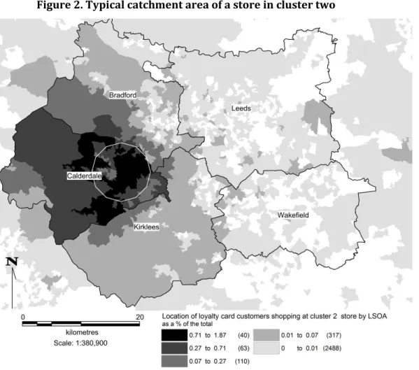
Cluster two is almost entirely made up of supermarket stores with the exception of one convenience store. This implies that this one convenience store experiences a trade profile more similar to supermarkets, hour-by-hour, throughout the day. We have labelled this cluster as traditional
supermarket Figure 2 shows the typical catchment area of a store in this cluster, again derived from actual customer patronage observed within our loyalty card dataset. In this case, the specific store is a supermarket in a major town in the Calderdale district. The catchment can be seen to be much more of a traditional residential nature, with a much sharper distance decay pattern than those seen in cluster one.
Cluster three has been labelled as typical convenience These stores tend to serve suburban and rural areas and also have very limited spatial extent to their catchment areas showing that they serve very local communities. As well as local residents, sales could also be influenced by other local demand sources such as schools or hospitals. We shall discuss more on this in the next section.
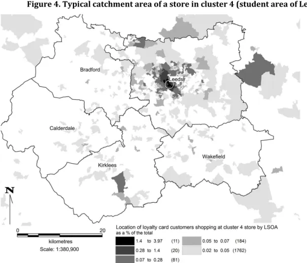
Cluster four is made up of only two convenience stores, both located in highly student centred suburbs, which offer a potential explanation of the peculiar store trading patterns shown in Figure 5. This profile is a little harder to explain fully. The bulk of sales do come from the immediate student catchment but the map shows some sales from individuals with an address far from the local vicinity. The loyalty card data used may give misleading patterns with some students registering their home address typically a non-residential parental address) rather than their term-time address.
Figure 4. Typical catchment area of a store in cluster 4 (student area of Leeds)
Table 4 shows the summary statistics for how far persons typically travel to the stores in each of the clusters. Research in the US has noted that families undertaking a grocery shop from home were reported to travel a median distance of 1.26 miles to do their shopping (Hillier et al., 2011). Similarly a space-time analysis of multi-purpose shopping (MPS) reported average distances of 1.8 and 3.9km for small and large shopping centres in Australia (Baker, 1996, Baker, 1994). The areas in close proximity to stores in this study support these findings, contributing the highest volumes of sales (£) (Table 4). However, evidence presented in Table 4 also demonstrates journeys far further than this, indicating that residential demand, localised around a supermarket, does not account for all sales at these stores. In some cases the observed, long distance, transactions could be the result of poor data quality: out of date residential addresses perhaps where customers have moved. However, it is unlikely this applies to
appear to indicate the existence of non-local/non-residential demand, comprising a number of individuals shopping some distance from home. This demand may be the result of workers shopping at stores in proximity to their workplace or commuting route. It may also comprise non-local residents that live outside the core catchment but travel further to shop at this store (see below), or other non-residents such as tourist and leisure populations.
Store catchment areas can be derived from the areal extent that a defined level of consumer patronage originates (Dolega et al., 2016). Following industry practice by our partner organisation, core catchment areas used in this study represent the spatial extent over which 70% of total store level sales are achieved. We present the core catchment areas on a cluster-by-cluster basis using a single catchment size (for all the stores in each cluster) and not drive times. Due to the predominant number of convenience stores, which are noted as having reduced levels of car borne trade (Wood and Browne, 2007), the use of drive times would not have been appropriate. Though all stores within a cluster are represented by a single catchment size, all stores have a unique catchment which is derived using actual loyalty card transactions and therefore catchment size will be representative of actual drive time behaviour exhibited by loyalty card holders. Cluster three (typical convenience) demonstrates a core catchment size of 2km, suggesting a strong link to fairly localised convenience shopping behaviour. Cluster two (traditional supermarkets) and one (workday convenience), on the other hand, have a core catchment of 5km. This is likely to be a function of these being bigger and more attractive stores, and a necessity to travel given the lack of residential populations in proximity to these stores or in cluster one being driven by commuters travelling to work from their homes. However, cluster two also demonstrates that a large proportion of their sales come from further afield, suggesting evidence of additional demand travelling to the store. Cluster four (student central) does not reach the 70%
threshold at any point in West Yorkshire suggesting that almost half of the cluster s sales come from
45+kms, which most likely represents loyalty cards registered to an alternative address as discussed above. However, loyalty card usage is registered for just 15% of the transactions undertaken at the two stores within this cluster suggesting that consumers are less motivated by brand loyalty. Where loyalty cards are used they demonstrate that customers are located in very close proximity to the store.
We have shown that store sales are not made up solely by local residents and in many cases some portion of sales originates from customers who have travelled to that store from outside of the typical core catchment. The proportion of sales accounted for by non-local demand and its spatial characteristics appears to vary by cluster. Hence, local and non-local demand are both important factors for store sales and the distances travelled by some consumers may offer insight into the types of demand involved. It is likely that the recorded transactions by consumers who have travelled further to a store may have made purchases as part of a multipurpose trip, combining several activities in one. In the next section we attempt to correlate these inferences with empirical demand data that demonstrate spatiotemporal fluctuations of different demand types, using this evidence to posit a connection
Table 4. Buffer analysis of cluster catchment areas using Loyalty card (LC) data
Cluster One - Avg. store size 2,915 (sqft) proportion of total sales (£) made from LC 31%
Buffer distance (km) % Of all loyalty card sales (£) Cumulative %1 of total loyalty card sales (£) Sales (% of total within 45km) Customer count (% of customers shopping in this cluster) Proportion of total res pop4 within
WY3 (%) Loyalty card representation of total population within WY (%)2 0 - 0.5 15.5 15.5 17.74 9.12 1.31 57.2 0.5 - 1 24.9 40.3 28.51 20.09 5 33.3 1 -2 19.9 60.3 22.83 23.31 14.03 13.6 2 - 5 13.5 73.7 15.43 21.37 31.08 5.6 5 - 10 6.9 80.7 7.96 13.07 24.79 4.3 10 - 15 3 83.6 3.41 6.18 15.19 3.4 15 - 20 0.9 84.5 0.98 1.69 5.69 2.4 20 - 45 2.7 87.2 3.14 5.17 2.99 14.2 Totals - 87.2 100 100 100 8.2
Cluster Two - Avg. store size 37,858 (sqft) - proportion of total sales (£) made from LC 50%
0 - 0.5 3.7 3.7 4.55 2.09 1.21 37.4 0.5 - 1 6.1 9.8 7.51 5.25 3.61 31.8 1 -2 19.4 29.2 23.9 17.02 12.45 28 2 - 5 42.8 72.1 52.69 48.26 51.44 19.5 5 - 10 1.7 73.8 2.1 18.14 22.96 16.1 10 - 15 4.5 78.3 5.56 5.2 6.16 18.3 15 - 20 1.2 79.5 1.45 1.46 2.25 14.4 20 - 45 1.8 81.3 2.24 2.57 0 0 Totals - 81.3 100 100 100 50.1
Cluster Three - Avg. store size 1,808 (sqft) proportion of total sales (£) made from LC 39%
0 - 0.5 33.7 33.7 34.22 19.73 2.82 43 0.5 - 1 26 59.6 26.39 21.39 4.57 28.8 1 -2 19 78.6 19.28 22.11 12.06 11.3 2 - 5 14.4 93.0 14.63 24.93 34.22 4.4 5 - 10 3.7 96.7 3.8 7.78 31.59 1.5 10 - 15 0.7 97.4 0.74 1.73 13.34 0.8 15 - 20 0.2 97.7 0.25 0.75 1.48 3.2 20 - 45 0.7 98.4 0.69 1.57 0 0 Totals - 98.4 100 100 100 6.1
Cluster Four - Avg. store size 1,797 (sqft) proportion of total sales (£) made from LC 15%
0 - 0.5 20.9 20.9 38.43 19.55 0.64 15.8 0.5 - 1 12.4 33.3 22.85 24.15 0.94 13.4 1 -2 6.9 40.2 12.67 15.73 1.98 4.2 2 - 5 6.5 46.6 11.87 18.84 12.48 0.8 5 - 10 2.4 49.1 4.48 8.17 15.93 0.3 10 - 15 1.3 50.4 2.44 4.04 22.23 0.1 15 - 20 1.3 51.7 2.44 2.99 18.31 0.1 20 - 45 2.6 54.3 4.81 6.53 27.57 0.1 Totals - 54.3 100 100 100 0.5
Buffer distances were designed to coincide with those used in-house by the retailers location analysis team.
1 The location analysis team consider a stores core catchment area to be indicated once a cumulative value of approximately 70% of sales (£)
is reached from the surrounding area.
2 Loyalty card representation is based on the proportion of total households represented by loyalty card customers in each buffer (assuming
that each household has only one registered loyalty card).
3 WY = West Yorkshire: which is represented at LSOA geography.
5. Temporal sales analysis
The availability of temporal data allows us to analyse the major sales fluctuations over a 24hr period. We demonstrate (Figure 5) the mean diurnal sales profile for stores within each of our four clusters at 30 minute intervals during a typical day. Most notably stores in cluster traditional supermarket exhibit a very different temporal sales profile to our other store clusters, with peak revenues accounted
for earlier within the day The temporal profile for stores in cluster workday convenience exhibits a
lunchtime and late afternoon peak, corresponding closely to previous research which noted increased convenience store sales at these times of the day in localities which experience large workplace populations (Berry et al., 2016). The sales fluctuations exhibited in Figure 5 are thus likely to be driven by the changing spatial patterns of demand as consumers go about their daily lives. While some consumer behaviour will be stochastic and therefore difficult to predict, the cluster analysis indicates that, at the aggregate level consumer behaviour demonstrates consistent temporal patterns at the store level. This was also observed on different days of the week. It seems that for the most part retail consumer behaviour is habitual, exhibiting recognised and predictable patterns at the aggregate level (Blythe, 2013, East et al., 1994, Solomon, 2013, Solomon et al., 2013).
Distinctive transitional periods in temporal sales are likely to be influenced by specific spatiotemporal demand side drivers, for example, lunchtime and late afternoon sales peaks experienced at stores in cluster 1 are likely to be driven by workplace demand. Where these peaks are observed in multiple clusters this couldbe the result of a particular demand type being present in both instances. The main transition points in temporal sales profiles (when sustained sales growth or decline typically occurs) are observed at the following approximate times across all clusters:
7am 11:30am (period of sales growth all stores) 11:30am 12:30pm (short period of rapid growth all stores)
12:30pm 2pm (period of sales decline all stores)
2pm 4/6:30pm (period of sales growth supermarkets/convenience) 4/6:30pm 12am (period of sales decline supermarkets/convenience)
Figure 5. Mean temporal sales profile by hour of the day for each cluster group, averaged across the whole week.
These transitional periods are clearly linked to the spatiotemporal nature of demand. For instance morning peaks are likely to be the result of workers or parents on the school run; the midday peak the result of a lunch time rush with workers buying food on their breaks; the afternoon period of reduced sales the result of limited customers because people are at home or at work; followed finally, by the peak in evening sales as people are leaving work or arriving home.
The afternoon period, although quiet in many stores, is interesting in that for certain stores there is a noticeable additional peak in the mid to late afternoon period (Figure 6). This is before many
people undertaking a traditional - working day finish work and so may be driven by a specific demand type or particular demand-side characteristics present within that store catchment at that time of the day. Given the timing and nature of the amenities within the specific store catchments we infer that this is driven by demand associated with school children or parents collecting children from school. Figure 6 shows two store profiles, which have this peak and are especially close to large secondary schools. This sharp rise, although not proportionally very large in terms of total store sales, appears in these stores around 1530 1700hrs correlating with the end of the school day and after school activities. While we cannot directly relate these sales to the presence of school based demand, the closeness of the schools certainly suggests localised fluctuations in sales at that point in day may indicate the impact of spatiotemporal school based demand. The same analysis was conducted on store sales for stores not located near school based demand and a similar rise in sales was not observed.
6 0 0 6 4 0 7 2 0 8 0 0 8 4 0 9 2 0 1 0 0 0 1 0 4 0 1 1 2 0 1 2 0 0 1 2 4 0 1 3 2 0 1 4 0 0 1 4 4 0 1 5 2 0 1 6 0 0 1 6 4 0 1 7 2 0 1 8 0 0 1 8 4 0 1 9 2 0 2 0 0 0 2 0 4 0 2 1 2 0 2 2 0 0 2 2 4 0 2 3 2 0 R e v e n u e Time of day 1 2 3 4
Figure 6. The uplift in sales 3-5pm for 2 partner stores close to major schools
Using the store level data it was also possible to re-examine the days of the week that consumers chose to shop (Table 5), providing an updated evaluation of grocery shopping days by consumers during the week and enabling a comparison to the earlier work of East et al. (1994) and the TUS. We observed an increased distribution in the share of shopping across the week. This could be a result of increased irregularity in working days and days off. At present, Fridays and Saturdays are the main shopping days, as found in East et al. (1994). Sundays appear to have become far more popular since East et al. (1994) study with an increase share of daily sales totals found in the TUS (Ipsos-RSL, 2003). This difference is likely in part due to changes in lifestyle and to the more liberal Sunday trading laws (De Kervenoael et al., 2006), introduced after East et al. (1994) study. This pattern, however, does not transfer into the convenience market and it is difficult to compare this to the previous evidence as the convenience market as it is today did not exist in the early 1990s (Hood et al., 2015). The data suggests that there is little variation in terms of the daily share of weekly sales in convenience stores suggesting that behaviour is often more consistent throughout the week. In addition, we also present the daily share of sales across each of the clusters, which include the same sample of stores.
Table 5. Daily share of the total weekly sales (%) by format and Cluster type
0 200 400 600 800 1000 1200 1400 1600 6 0 0 6 4 0 7 2 0 8 0 0 8 4 0 9 2 0 1 0 0 0 1 0 4 0 1 1 2 0 1 2 0 0 1 2 4 0 1 3 2 0 1 4 0 0 1 4 4 0 1 5 2 0 1 6 0 0 1 6 4 0 1 7 2 0 1 8 0 0 1 8 4 0 1 9 2 0 2 0 0 0 2 0 4 0 2 1 2 0 2 2 0 0 2 2 4 0 2 3 2 0 S a le s (£ ) Time of day
Store category Monday Tuesday Wednesday Thursday Friday Saturday Sunday Grand Total
All Stores 12.7 12.4 12.4 14.4 18.2 19.1 10.8 100 Supermarkets 10.7 10.2 10.3 12.2 15.5 16.6 8.5 84 Convenience 2.1 2.2 2.1 2.2 2.7 2.5 2.3 16 1 14.3 14.2 13.4 14.0 16.9 15.9 11.4 100 2 12.5 11.9 12.1 14.6 18.6 20.0 10.3 100 3 12.9 13.6 13.4 13.5 17.3 15.8 13.4 100 4 13.0 13.6 12.9 12.9 16.0 16.6 14.9 100
Given that spatiotemporal fluctuations in demand are important in understanding sales, to aid new store revenue prediction it would be useful to create a series of demand layers relating to the spatiotemporal distribution of demand at different times of the day. Home and work are clearly two important locations. The Census can provide data on residential populations as standard, representative of the night time population of an area, as this is noted to be one of the few times when the majority of the population are at home.
Workplace demand in England and Wales can be derived using census based Workplace Population Statistics. These are a new set of population statistics based on respondents self-reported employment status and workplace location and are disseminated using a custom-built geography workplace zones, which have been specifically created to account for the spatial distribution of workplace populations (Mitchell, 2014). We use counts of workplace populations (by workplace zone) as our indicator to represent this subset of the non-residential population.
We also capture the daytime population at their place of residence (not to be confused with the workday population available as a Census-derived population base (Bradley, 2014)). Our daytime population captures the usually resident population who remain at home during the day, (such as retirees or unemployed individuals). It has been derivedby subtracting the total count of people who depart that area from the census based usual resident population. Thus we subtract those individuals working elsewhere (as captured by our workplace population) and those that are at non-residential locations associated with study or leisure (as discussed below). We do not use the workday population count as this includes a count of workers commuting into a given area. In this instance we wish to disentangle the components that make up the daytime population and therefore capture separately those workplace populations and the residents that remain at home during the day. These shifting dynamics are important to accurately represent the distinction between night time and day time populations, in order for us to fully capture the components that drive retail demand fluctuations.
Data related to other components of demand need to be pieced together from scratch. If schools are deemed to offer a considerable sales uplift between 3 and 5pm (as suggested above) then it is useful to estimate the geography of the school-based population. School based demand can be first calculated by taking the total count of children aged between 11-15 who are in compulsory education and the total count of 16-17 year olds who reported themselves, at the time of the 2011 census, as full time students living at their place of residence. These individuals represent potential demand outflow and can be reallocated from their residential origins to their daytime places of study. The day time count of school based demand are a direct representation of the total number of secondary school students on the roll at each school in West Yorkshire this represents inflows. School based demand is reallocated to
schools based on the total number of school places available in the area School s locations are used as
the spatial component viathe LSOAthat it lies within. If the total capacity for school children is reached in any given LSOA then it is assumed that the additional outflows represent students who attend
schools in nearby LSOAs. If on the other hand the outflows do not exceed the total school pupil capacity then it is assumed additional pupils from outside of the study region contribute to the inflow, ensuring that the reported total pupils on the roll is always achieved. The temporal component of student populations can be derived by the typical UK school hours (approximately 9am-3:30pm during term time), allocating students to school within these hours and at home outside of them.
For cluster 4 Student Central , university student demand seems crucial and can be derived from two sources: first the usual place of residence of students ascertained using the 2011 census. The data used represents a total count of the usual residential population of 18+ year olds who declared themselves as students. This includes students who live at a parental home during term time or those who live at an alternative term time address (such as a university hall of residence). We classify this address as the usual place of residence, represented at the LSOA level (ONS, 2011, ONS, 2014a, ONS, 2014b). Second, data providing counts of student enrolment at universities was obtained from the Higher Education Statistics Agency (HESA). This provides total counts of higher education students, by
higher education provider using the university s postal address as a spatial reference for their daytime location. We suggest an initial temporal distribution for students according to the following framework: 10% (at home) and 90% (on campus) split. This framework has been adapted from the findings of Edwards and Bell (2013), who suggest that (in an Australian context) an approximate figure of 90% of total university population was found on campus around midday during term time, following the results of a survey of campus populations.
There may be other drivers of spatiotemporal demand fluctuations, especially those which may be experienced at a very localised level and impact on specific grocery convenience stores. These may include leisure and tourist populations, plus those attending major events. Leisure is a growing component of our present day society, contributing large quantities of expenditure into economies (Au and Law, 2002, Song and Li, 2008). We have therefore considered the potential for spatiotemporal demand fluctuations to be driven by populations at major West Yorkshire visitor attractions. This is only an indicator of one proportion of leisure demand and has been derived from VisitEngland, the destination management organisation responsible for promoting England as a tourist destination and undertaking related research and development. It represents a count of visits to the top twenty (paid and free) visitor attractions in Yorkshire and the Humber, from which we have extracted those located within our West Yorkshire study area (Visit England, 2015, VisitEngland, 2015). Data availability detailing surveyed visitor numbers, such as visits to family and friends or day visits, where reported are typically presented over larger geographic scales and often sources are aggregated together, such as in The GB Day Visits Survey 2015, which does not provide geographical detail below the Local Authority District (LAD) level (Orrell et al., 2015). Qualitative data detailing explicit counts of visitors at a destination level, in addition to the amount they spend on groceries, are hard to come by (Downward and Lumsdon, 2000, Newing et al., 2014a). Therefore only the number of weekly visitors to top
from the arrival of visitors to an areaas this included explicit counts of visitors and was vitally spatially referenced by the location of the attraction (excluding other forms of leisure visitors from this study). It is difficult to try to understand store level sales fluctuations within highly localised catchment areas when using aggregate regional figures as local level change may vary considerably and not be representative of a region.
Table 6 provides a summary of the data that has been used to construct these different demand layers. This represents a bottom-up approach to building the demand layers and while this may limit the immediate feasibility of location planning teams implementing a similar demand layering due to lacking resources (Wood and Reynolds, 2011), in order to fully understand the contribution of each demand type it was important to build it from the bottom up. However, data availability is constantly improving and could permit inclusion of these forms of demand within a retail modelling framework. The provision of Workplace Population Statistics and custom small-area geography following the 2011 Census enables inclusion of these populations. Similarly, increases in the provision of open data (for example related to school rolls and catchment areas) provide increasingly (albeit fragmented) sources which retailers could use to build some of these demand layers. Commercial data aggregators and consultancies have begun to repackage these open data sources into user-friendly formats suitable for these forms of analysis. Geolytix, a UK based consultancy (https://www.geolytix.co.uk/?geodata), provide datasets related to transport interchanges, educational establishments, workplaces and points of interest which could support in-house retail location-based modelling of this nature. .
Table 6. Summary of Temporal demand database
Tables 7 and 8 (shown below) show counts and proportions of each demand group within the core catchment area around each of the store clusters for both night and day phases. Table 7 demonstrates the total count of residential populations at night. The traditional residential count accounts for all of the registered population living in each catchment area, represented by their home addresses (the likely location that they reside in overnight). Table 8 demonstrates the total estimated count of daytime populations within each catchment area. This time population count is based on the locations that populations are inferred to be present at during the day and includes workplace, leisure, school and university as key drivers of the spatial and temporal distributions of these populations.
In Figures 7 and 8 we demonstrate the spatiotemporal component of these demand side estimates. We loosely define two time periods midday (Figure 7) and night time (Figure 8). Using the Leeds LAD as an example of the analysis across West Yorkshire, we observe notable differences in the geography of demand between the two time periods. There appears to be a considerable shift towards
Demand name Demand type Data source Description
Residential demand
Total residents 2011 Census Count of total population census
variable KS101EW Daytime residents at place of residence 2011 Census
Estimated daytime residential
population (derived from the
remaining residents following the removal of school, university and workplace demand)
School based demand
At home 2011 Census
Number of secondary school age
children in the population - census
variable DC1106EW
At school
Department for Education s Schools, pupils and their
characteristics (2016)
Number of secondary school pupils enrolled at schools in West Yorkshire
University demand
At home 2011 Census
Number of full time students aged 18+ living at home or a term time
address - census variable
DC1106EW
On campus
Higher education students, by higher education provider: Higher Education Statistics Agency (HESA), (2015)
Number of enrolled students at higher education providers in West Yorkshire
Workplace
demand At workplace
2011 Census Workplace Population statistics
Number workers at their registered place of work (including from home) by Workplace Population Zone.
Leisure demand
Daytime visitors
Annual survey of visits to visitor attractions
Average number of weekly visitors to the top 20 paid and free
attractions in Yorkshire and Humber (2015)
the city centre during the day (Figure 8) with highly localised clustering of demand types throughout the Leeds area, with noticeable clusters associated with workplace and university populations.
If we are to improve revenue estimations in the future for the stores within the different clusters, it is important to use these time demand profiles in those forecasts so that we allocate the correct type of demand from where it originates during the day, a point we reflect on further below.
Table 7. Count of demand types overnight within the core catchment area each cluster group of stores
Table 8. Count of demand types during the day within the core catchment area for each cluster group of stores Core
catchment (km)
Cluster group
Night time residential demand
Total residential population Resident count:
Non-student/unemployed or retired Presence (% of total) University demand count Presence (% of total) School based demand count Presence (% of total) Employed resident count Presence (% of total) 5 1,2 1 574907 493 81372 7 113667 10 408378 35 1178324 5 1,2 2 745839 493 88828 6 142687 9 548622 36 1525976 21,2 3 196579 473 38164 9 35465 8 149367 36 419575 1 4 5451 13 22802 533 1221 3 13772 32 43246 Core catchment (km) Cluster group
Total residential count Residential demand University demand School based demand Workplace demand Leisure demand
Total day time count Traditional night time population Presence (% of total) Day time demand at place of residence Presence (% of total) At residence4 Presence (% of total) On Campus4 Presence (% of total) At school Presence (% of total) At Workplace Presence (% of total) At Attractions Presence (% of total) 5 1,2 1 1178324 85 574907 42 8137 1 62771 5 81044 6 616789 453 40575 3 1384223 5 1,2 2 1525976 89 745839 443 8883 1 73215 4 101641 6 749401 443 29600 2 1708579 21,2 3 419575 78 196579 37 3816 1 28980 5 20696 4 276466 513 11825 2 538362 1 4 43246 92 5451 12 2280 5 27927 603 387 1 10749 23 0 0 46794
1 Core catchment defined by distance that a total of 70% of sales is achieved. 2 Proportion of demand type within core catchment (% of total).
3 Main demand group based on total volume in core catchment (% of total).
4 Estimates of university demand are based on a survey identifying the proportion of students on campus throughout the day. Values are based on midday estimates reaching around 90% of the total (Charles-Edwards and Bell, 2013).
Figure Spatiotemporal representation of midday demand populations for Leeds LAD at LSOA level (workplace populations have been overlaid using Workplace Population Zones)
Figure Spatiotemporal representation of nighttime demand populations for Leeds LAD at LSOA level.
6. Conclusions
In this paper we have demonstrated how grocery store sales fluctuate through the day and we have provided evidence, which appears to indicate that these fluctuations are driven by spatiotemporal fluctuations on the demand side. It is clear that at certain points during the day there are considerable shifts in the spatial distribution of consumers. The existence of spatiotemporal fluctuations in demand has been shown using rarely available store trading data and loyalty card records related to consumer behaviours. Much of these data indicate that demand is likely not to always originate from a given consumer's residential home address but also from work-based locations, schools, universities and perhaps leisure destinations. As grocery retailing diversifies into new formats and location types, it is important to understand the spatial and temporal nature of demand and its localised store-level impact on the supply side. This was shown in our cluster analysis where it became apparent that stores grouped together (based on their temporal sales profile) demonstrated analogues in terms of the spatiotemporal demand patterns within the store core catchment.
Critically, these valuable and novel findings could offer retailers innovative opportunities to support their store location planning process. This should enable them to move beyond conventional analogue approaches by building these demand types into a modelling framework, which would enable them to predict the types of sales profile that may be expected in a store when developing new sites. This has clear implications for strategic decision making and in day-to-day operational concerns such as staffing, stocking and store layout policies. From a practical point of view, this would be particularly useful for a new store, allowing retailers to consider staffing optimisation, product ranges and store format at the planning stage of new store development. The impact of this insight could also be developed further by retailers by combining time stamped product sales data, combining the types of products bought at certain times of day with the cluster profiles. Combining this data could add additional layers of detail and provide an interesting insight into spatiotemporal consumer shopping behaviours at the product category level. Furthermore, practical implications for Food for now type offers could be administered uniquely to stores varying spatially, store-by-store and temporally, hour-by-hour and could allow retailers to employ promotions dynamically throughout the day, actively responding to, and predicting, varying demand. Moreover, retailers would be able to optimise new and existing stores effectively, dealing with key operational costs such as staffing by responding to temporal changes experienced by stores as demonstrated in the clusters and focusing a stores mission to cater to the demand types available, e.g. workers or school pupils.
Understanding the temporal dynamics of demand and how this affects store sales is of crucial importance to retailers. Therefore, they represent important factors to address when undertaking modelling techniques and sales forecasting (Birkin et al., 2013). The incorporation of additional demand layers and spatiotemporal extensions into location planning models has the potential to improve the accuracy of store sales predictions considerably (Newing et al., 2013a, Newing et al., 2013b, Newing et
continually lead to underestimations in sales and store performance modelling in certain locations. Commercially, the impact of time is yet to be fully explored and while some retailers are beginning to examine short-term changes in demand and the impact at a store level, for instance local events or the weather, there has been little attempt to incorporate these at a more strategic level for sales predictions (Newing et al., 2013a). We are aware of the challenging organisational issue facing location-planning teams, such as struggling for internal legitimacy as new store development has declined, through our close association with our data partner. We believe that the clustering framework developed in this paper has the potential to generate a high level of commercial interest when used in a predictive capacity. We have demonstrated that there are habitual and observable patterns in temporal sales and groups of stores with similar characteristics were also noted. We believe from a commercial perspective that not only has this never been done before (regarding temporal sales profiles), but that here lies the commercial interest. This is particularly important for modelling in the grocery sector. Retailers use modelling for location planning, performance monitoring and sales predictions. In many cases models are overly simplistic and fail to accurately capture more complex temporal conditions. Hence, current modelling frameworks using static populations are likely to remain limited when applied to stores and location types where non-residential demand represents a considerable driver of sales. We suggest future research is needed to include temporal extensions and the next step in our research is to supplement these novel analyses through the incorporation of these forms of spatiotemporal demand within a refined spatial interaction model, currently widely used in the UK grocery sector for store revenue estimation and impact assessment (Reynolds and Wood, 2010). Results of these modelling extensions and analyses will be reported in future papers.
References
ARENTZE, T.A., BORGERS, A. AND TIMMERMANS, H., 1993. A model of multi purpose shopping trip behavior. Papers in Regional Science, 72(3), 239-256.
ARENTZE, T.A., OPPEWAL, H. AND TIMMERMANS, H.J., 2005. A multipurpose shopping trip model to assess retail agglomeration effects. Journal of Marketing Research, 42(1), 109-115
AU, N. & LAW, R. 2002. Categorical classification of tourism dining. Annals of Tourism Research, 29, 819-833.
BAKER, R. G. 1994. An Assessment of the Space Time Differential Model for Aggregate Trip Behavior to Planned Suburban Shopping Centers. Geographical Analysis, 26, 341-363.
BAKER, R. G. 1996. Multi-purpose shopping behaviour at planned suburban shopping centres: a space-time analysis. Environment and Planning A, 28, 611-630.
BELL, M. 2015. Demography, time and space. Journal of Population Research, 32, 173-186. BENOIT, D. & CLARKE, G. 1997. Assessing GIS for retail location planning. Journal of retailing and
consumer services, 4, 239-258.
BERRY, T., NEWING, A., BRANCH, K. & DAVIES, D. 2016. Using workplace population statistics to understand retail store performance The International Review of Retail, Distribution and Consumer Research, 1-21.
BIRKIN, M., HARLAND, K. & MALLESON, N. 2013. The classification of space-time behaviour patterns in a British city from crowd-sourced data. Computational Science and Its Applications ICCSA 2013.
Springer.
BIRKIN, M. & MALLESON, N. 2013. Investigating the Behaviour of Twitter Users to Construct an
Individual-Level Model of Metropolitan Dynamics. Working paper. National Centre for Research methods.
BLYTHE, J. 2013. Consumer behaviour, London, SAGE.
BRADLEY, A. 2014. 2011 Census:Workplace Population Analysis. Available online at
-https://www.ons.gov.uk/peoplepopulationandcommunity/populationandmigration/pop
ulationestimates/articles/workplacepopulationanalysis/2014-05-23:
Office of National Statistics.CHARLES-EDWARDS, E. & BELL, M. 2013. Estimating the service population of a large metropolitan university campus. Applied Spatial Analysis and Policy, 6, 209-228.
CLARKE, G., EYRE, H. & GUY, C. 2002. Deriving indicators of access to food retail provision in British cities: studies of Cardiff, Leeds and Bradford. Urban Studies, 39, 2041-2060.
DE KERVENOAEL, R., HALLSWORTH, A. & CLARKE, I. 2006. Macro-level change and micro level effects: A twenty-year perspective on changing grocery shopping behaviour in Britain. Journal of Retailing and Consumer Services, 13, 381-392.
DOLEGA, L., PAVLIS, M. & SINGLETON, A. 2016. Estimating attractiveness, hierarchy and catchment area extents for a national set of retail centre agglomerations. Journal of Retailing and Consumer Services, 28, 78-90.
DOWNWARD, P. & LUMSDON, L. 2000. The demand for day-visits: an analysis of visitor spending.
Tourism Economics, 6, 251-261.
EAST, R., LOMAX, W., WILLSON, G. & HARRIS, P. 1994. Decision Making and Habit in Shopping Times.
European Journal of Marketing, 28, 56-71.
EVERITT, B., LANDAU, S. & LEESE, M. 2001. Cluster analysis, New York;London;, Arnold. HARRIES, J. 2014. Growing UK convenience market. The Institute of Grocery Distribution.
HILLIER, A., CANNUSCIO, C. C., KARPYN, A., MCLAUGHLIN, J., CHILTON, M. & GLANZ, K. 2011. How far do low-income parents travel to shop for food? Empirical evidence from two urban neighborhoods.
Urban Geography, 32, 712-729.
HOOD, N., CLARKE, M. & CLARKE, G. P. 2015. Segmenting the growing UK convenience grocery market for store location planning. International Journal of Retailing, Distribution and Consumer Research.
HORNIK, J. 1984. Subjective vs. objective time measures: A note on the perception of time in consumer behavior. Journal of Consumer Research, 615-618.
IPSOS-RSL 2003. United Kingdom Time Use Survey, 2000, [data collection]. UK Data Service. Office of National Statistics.
LANGSTON, P., CLARKE, G. P. & CLARKE, D. B. 1997. Retail saturation, retail location, and retail competition: an analysis of British grocery retailing. Environment and Planning A, 29, 77-104. LOVELACE, R., CLARKE, M., CROSS, P. & BIRKIN, M. 2015. Verification of big data for estimating retail
flows: A comparison of three sources against model results. Geographical Analysis.
MALLESON, N. & BIRKIN, M. 2013b. Estimating Individual Behaviour from Massive Social Data for An Urban Agent-Based Model. In: KOCK, A. & MANDL, P. (eds.) GeoSimulation: Modeling Social Phenomena in Spatial Context. Germeny: Lit Verlag.
MALLESON, N. & BIRKIN, M. New Insights into Individual Activity Spaces using Crowd-Sourced Big Data. Proceedings of IEEE Big Data Science, 2014 Berkeley.