Empirical evaluation of Soft Arc Consistency algorithms for solving Constraint Optimization Problems

(1)

Empirical Evaluation of Soft Arc Consistency

Algorithms for Solving Constraint

Optimization Problems

A Thesis Submitted to the

College of Graduate Studies and Research

in Partial Fulfillment of the Requirements

for the degree of Master of Science

in the Department of Computer Science

University of Saskatchewan

Saskatoon

By

Xiaonuo Gantan

c

(2)

Permission to Use

In presenting this thesis in partial fulfilment of the requirements for a Postgraduate degree from the University of Saskatchewan, I agree that the Libraries of this University may make it freely available for inspection. I further agree that permission for copying of this thesis in any manner, in whole or in part, for scholarly purposes may be granted by the professor or professors who supervised my thesis work or, in their absence, by the Head of the Department or the Dean of the College in which my thesis work was done. It is understood that any copying or publication or use of this thesis or parts thereof for financial gain shall not be allowed without my written permission. It is also understood that due recognition shall be given to me and to the University of Saskatchewan in any scholarly use which may be made of any material in my thesis.

Requests for permission to copy or to make other use of material in this thesis in whole or part should be addressed to:

Head of the Department of Computer Science 176 Thorvaldson Building 110 Science Place University of Saskatchewan Saskatoon, Saskatchewan Canada S7N 5C9

(3)

Abstract

A large number of problems in Artificial Intelligence and other areas of science can be viewed as special cases of constraint satisfaction or optimization problems. Various approaches have been widely studied, including search, propagation, and heuristics. There are still challenging real-world COPs that cannot be solved using current methods.

We implemented and compared several consistency propagation algorithms, which include W-AC*2001 (Cooper and Schiex, 2004), EDAC (Givry and Zytnicki, 2005), VAC (Cooperet al., 2010), and xAC (Horschet al., 2002). Consistency propagation is a classical method to reduce the search space in CSPs, and has been adapted to COPs. We compared several consistency propagation al-gorithms, based on the resemblance between the optimal value ordering and the approximate value ordering generated by them. The results showed that xAC generated value orderings of higher quality than W-AC*2001 and EDAC.

We evaluated some novel hybrid methods for solving COPs. Hybrid methods combine consis-tency propagation and search in order to reach a good solution as soon as possible and prune the search space as much as possible. We showed that the hybrid method which combines the variant TP+OnOff (Section 3.3) and branch-and-bound search (Section 3.5) performed fewer constraint checks and searched fewer nodes than others in solving random and real-world COPs.

(4)

Acknowledgements

There are many people who deserve my sincere gratefulness. In particular, I want to thank Dr. Michael C. Horsch for his excellent supervision, patient guidance, unconditional support, and sparking inspiration throughout my graduate studies. Many thanks are due to the other supervisory committee members: Dr. Anthony J. Kusalik and Dr. Kevin Stanley.

(5)

This is the thesis is dedicated to my father, who set up an example for me on how to be consistent and devoted to my work. It is also dedicated to my mother, who loved me unconditionally and supported me no matter how hard the graduate studies are.

(6)

List of Tables

6.1 Storage Costs . . . 65

6.2 Shipment Cost . . . 66

6.3 Unary Constraints for Warehouses . . . 66

6.4 Unary Constraints for Stores . . . 66

6.5 UWLP instances . . . 67

6.6 Number of Constraint Checks on UWLPs . . . 68

6.7 RLFAP Instances . . . 74

6.8 Number of Constraint Checks for Solving RLFAPs . . . 75

6.9 Number of Nodes Searched for Solving RLFAPs . . . 75

(9)

List of Figures

2.1 An example of search tree including two variables . . . 8

2.2 Structure of a Constraint . . . 21

2.3 An Example of Combination and Projection . . . 22

2.4 From SCSP to VCSP . . . 24

2.5 From VCSP to SCSP . . . 25

3.1 A WCSP instance that is notN C∗ . . . 32

3.2 A WCSP instance that isN C∗ . . . 33

3.3 A WCSP instance that isDAC∗ . . . 33

3.4 A WCSP instance that isAC∗ _{but not}_DAC∗ _{. . . 34}

3.5 A WCSP instance that isF DAC∗ _{but not}_EDAC∗ _{. . . 39}

3.6 A WCSP instance that isEDAC∗ _{. . . 40}

3.7 The parameters of an arbitrary node X . . . 43

4.1 Two Binary Constraints in A Skewed COP Instance . . . 52

4.2 Quality Comparison of Value Ordering Heuristics . . . 55

5.1 Comparing Number of Constraint Checks on MaxCSPs . . . 57

5.2 Comparing Number of Nodes on MaxCSPs . . . 58

5.3 Comparing Number of Constraint Checks on UICOPs . . . 60

5.4 Comparing Number of Nodes on UICOPs . . . 60

6.1 Binary Constraints . . . 67

6.2 Number of Constraint Checks Performed for Solving Quasigroups . . . 80

(10)

List of Abbreviations

AC Arc Consistency

ACS Arc Consistency during Search

BJ Backjumping

BM Backmarking

BnB Branch and Bound BT Backtracking

CARD Minimum Cardinality CP Consistency Propagation CS Constraint System

CSP Constraint Satisfaction Problems COP Constraint Optimization Problems DAC Directional Arc Consistency EAC Existential Arc Consistency

EDAC Existential Directional Arc Consistency FDAC Full Directional Arc Consistency FEAS Feasibility

GI Generalized Interval GT Generate and Test MAX Maximum Feasibility

MaxCSP Max Constraint Satisfaction Problems MSAC Maintaining Soft Arc Consistency NC Node Consistency

NP Non-deterministic Polynomial-time PCC Pearson’s Correlation Coefficient QCP Quasigroup Completion Problem QWH Quasigroup With Holes

RLFAP Radio Link Frequency Assignment Problem RP Radical Pruning

SAC Soft Arc Consistency

SCSP Semiring-based Constraint Satisfaction Problems SPAN Minimum Span

SRCC Spearman’s Rank Correlation Coefficient TP Tree Pruning

UICOP Uniform Integer Constraint Optimization Problem UWLP Uncapacitated Warehouse Location Problem VAC Virtual Arc Consistency

VCSP Valued Constraint Satisfaction Problems W-AC*2001 Weighted Arc Consistency 2001

(11)

Chapter 1 Introduction

Constraint satisfaction problems (CSPs) and constraint optimization problems (COPs) include many real-world applications in machine vision, belief maintenance, scheduling, and others. Be-cause of the various applications in which CSPs and COPs are useful, extensive research has been devoted into developing more efficient algorithms for solving them. After decades of hard work by researchers, the understanding of CSPs and the development of algorithms have brought ben-efits to the real world. The practical application of COPs, however, still have lots of questions waiting to be answered. Based on one of the popular COP frameworks, this thesis concentrates on improving the performance of the xAC algorithm (Horschet al., 2002), and aims at providing comprehensive empirical results by comparing different state-of-the-art algorithms based on their empirical performance.

A CSP includes a set of variables, a finite and discrete domain for each variable, and a set of constraints. Each constraint is a subset of the Cartesian product of all the domains of some variables. The goal is to find an assignment of values to all the variables such that this assignment satisfies all the constraints. This assignment is called a solution to the problem. On the other hand, if there is no such assignment, the problem has no solution. Typically, we stop when we find a solution, but we may want to find all solutions for some problems.

Constraints are classified as unary, binary, or n-ary constraints, based on the number of variables involved. A unary constraint includes only one variable, and prevents some of the values in the domain from being assigned to the variable. Similarly, a binary constraint includes two variables, and prohibits some illegal assignments of value combinations. The COP instances in this thesis contain only unary or binary constraints, because anyk-ary (k >2) constraints can be converted

(12)

to several binary constraints.

The following is an example of constraint satisfaction problem. Establishing a network of radio links gives rise to the Radio Link Frequency Assignment Problem (RLFAP) (see Page 70). A radio link is a communication channel between a pair of radio transmitters. A signal can be transmitted through a radio link from one transmitter to the other. Each radio link must be assigned an operating frequency from a set of available frequencies. The distance between links is measured by the difference of the frequencies assigned to them. The assignment complies with certain preferences, regulations, and physical locations of the transmitters. First, some links may have preassigned frequencies. Second, when two transmitters each of which hosts a different link are physically close to each other, the difference of these two frequencies have to be large enough so the communication is not distorted. Third, each link has a reverse link. A reverse link allows simultaneous transmission between transmitters. The frequencies assigned to each reverse link have to differ from the original link by a certain distance. A link and its reverse link occur in pairs.

A radio link frequency assignment problem can be modelled as a CSP by declaring each radio link as a variable (Cabonet al., 1999; Freuder and Wallace, 1992). The domain of each variable is the set of available frequencies for that link. Unary constraints specify preassigned frequencies. Binary constraints specify that the frequencies assigned to any two links should be different from each other by a certain amount. To solve an RLFAP is to find an assignment of all the links that comply with all the constraints.

Based on the current constraint satisfaction framework, an RLFAP can be solved by various methods, including tree search, local search, consistency propagation, and heuristics (see Chapter Two). No matter which method is chosen, the constraint satisfaction framework allows certain flexi-bility to deal with different problem instances. For example, with some possible minor modifications, altering the preassigned frequencies and the smallest distance between each pair of interfering link assignments will not require changing the solving technique, although the solution of the problem may change.

(13)

CSP can be over-constrained where no solution exists. For example, in an RLFAP, if the originally assigned frequency of the link in one direction has to differ from the reverse one by a large distance, there may be no assignment satisfying all constraints.

In order to effectively solve over-constrained CSPs, each constraint is associated with violation costs (Schiexet al., 1995; Bistarelliet al., 1999). These associations transform CSPs into COPs, which can be solved by finding an assignment that minimizes the total costs of all violated con-straints. The costs or weights indicate the preference or importance over different constraints, thus the assignment minimizing the costs is the most preferable one. These costs or weights are part of problem descriptions and are assessed by domain experts. Considering a radio link frequency problem, if the hard constraints between some links cannot be broken under all conditions, while the soft constraints between other links can be broken for a certain cost, then the final solution satisfies all the hard constraints and violates as few soft constraints as possible.

Constraint optimization algorithms are built on top of constraint satisfaction techniques, and constraint optimization frameworks extend constraint satisfaction models. Because of the valua-tion of each partial assignment and the comparison between different assignments, the computa-tional complexity of COPs is higher than CSPs (Cohenet al., 2006). Since the time complexity of COPs is nondeterministic polynomial, more efficient algorithms are needed. Most of the cur-rent COP algorithms are developed by extending their counterparts in solving CSPs. The popular options include branch-and-bound Search, Russian Doll Search (Verfaillieet al., 1996), Partial Con-sistency Propagation (Verfaillieet al., 1996), and Soft Node and Arc Consistency (Larrosa, 2002; Cooper and Schiex, 2004; Cooperet al., 2010).

In this thesis, the major part of the work is devoted to developing more efficient heuristic inference algorithms which generate value orderings to guide the branch-and-bound search, and comparing our heuristic algorithms against various state-of-the-art consistency propagation algo-rithms. The algorithm we improved is xAC (Horschet al., 2002). Since xAC and other algorithms only generate value ordering and perform consistency propagation without any search, we com-bined these algorithms with a plain branch-and-bound search and compared the performance of

(14)

the hybrid algorithms. The branch-and-bound algorithm is introduced by Land and Doig (1960). A summary of this thesis is:

• Study of consistency propagation (CP) and value ordering heuristics in a COP framework;

• Implementation of W-AC*2001, EDAC, VAC, xAC and variable ordering heuristics combined with a branch-and-bound search algorithm;

• Proposal of several xAC variations (Section 3.3) to guide the search;

• Extensive empirical comparisons of different hybrid algorithms for both random and real-world COP solving;

• Analysis of the performance of using different parameters for the xAC algorithm.

This is the first work that systematically studies the value ordering heuristic provided by xAC and different xAC variations in a branch-and-bound search for solving COPs. It is also the most extensive work to explore the potential of the xAC algorithm.

The rest of this thesis is structured as follows. Chapter 2 gives a literature review of the back-ground and the related work on CSP/COP frameworks and the algorithms. Chapter 3 introduces a group of so-called “soft” AC properties (Cooper and Schiex, 2004) and propagation algorithms. Chapter 4 gives a comparison of the value ordering heuristics generated by xAC, W-AC*2001, and EDAC. Chapter 5 shows an empirical comparison of xAC, EDAC, and VAC on solving random COPs. Chapter 6 compares the xAC, EDAC, and VAC on solving several real world COPs.

(15)

Chapter 2 Literature Review

This chapter gives a brief description of the frameworks for modelling CSPs and COPs and relevant arc consistency algorithms. Section 2.1 introduces the classical CSP framework. Section 2.2 introduces classical CSP algorithms. Section 2.3 introduces two popular COP frameworks, valued CSPs (Schiexet al., 1995) and semiring-based CSPs (Bistarelliet al., 1999), which are used to model weighted CSPs.

2.1 Constraint Satisfaction Framework

Definition 2.1. Constraint Satisfaction Problem (CSP). A Constraint Satisfaction Problem is a tuple P= (X, D, C), where

• X ={x1, x2,· · · , xn} is a set of variables;

• D ={d1, d2,· · · , dn} is a set of finite domains, each di contains values{v1, v2,· · ·, vk} that

can be assigned to variable xi, where kis an integer that may be different for different i;

• C is a set of constraints, each of which allows some simultaneous assignments of some val-ues to certain variables and forbids the rest. Each constraint is a subset of the total carte-sian product of all the domains of involved variables: for constraint ci defined over variables

xi₁, xi₂,· · · , xij,ci⊂di1×di2× · · · ×dij.

Each variable in X has a corresponding domain in D, which contains a set of distinct values. Any of these values can be assigned to this variable.

An example of CSP is scheduling a birthday party time. Each guest has his or her own schedules. Some of them may work night shifts, while others work during the day. What is the best time so

(16)

that everyone can join the party? In this case, the set of variables would be X = {x1,· · ·, xn}

where xi is a potential party guest. The set of domains would beD={d1,· · · , dn} where di is a

set of time slots when xi is available. The set of constraints would beC ={c1, c2,· · ·, cn}, where

ciforbids certain time slots being assigned to xi because the guestiwill not be available for those time slots. Such a small question can be answered by manually selecting a time slot when all guests are available. However, if it is a shareholders’ meeting about a company’s annual financial report, it might be hard to find the perfect time slot so that all significant shareholders can attend the meeting. When the number of people involved becomes bigger and bigger, a good algorithm for solving general CSPs will save a lot of time and effort.

The following overview is based on binary CSPs, in which C only contains unary and binary constraints. A unary constraint involves only one variable and a binary constraint involves two. Similarly aN-ary constraint prohibits certain value assignments betweenN variables. Since N-ary (N >2) constraints can be transformed into binary constraints, we restrict our attention to binary constraints without loss of generality (Bacchus and Beek, 1998) .

The goal of solving CSPs is to assign a valuevto each variablexsuch that the whole assignment satisfies all the constraints. Such an assignment is called a solution. All the possible assignments form the Cartesian product of all the domains: D = d1 ×d2× · · · ×dn. Because the size of

the Cartesian product grows exponentially with the number of variables, a brute force algorithm searching all possibilities to find the optimal answer is impractical and we need intelligent algorithms to prune unnecessary search.

Several necessary definitions to formalize CSPs are defined as follows (Dechter, 1990).

Definition 2.2. Constraint . A Constraint ci is a relation ri defined on a subset of variables

si ⊆X. The relation denotes the variables’ simultaneous legal value assignments. si is called the scope of ri.

If si = {xi₁,· · · , xir}, then ri is a subset of the Cartesian product di1 × · · · ×dir. Thus, a constraint can also be viewed as a pairci=hsi, rii.

(17)

of a valuev∈di toxi; a partial assignment of a set of variablesY ∈Xis a set of single assignments for each variable inY; a full assignment is a partial assignment whose set of variables is equal toX. A partial assignment is consistent if it satisfies all of the constraints whose variables are assigned.

Definition 2.4. Solution . A solution is a full assignment such that ∀c ∈ C, c is satisfied by a partial assignment whose set of variables Y is a subset of X.

2.2 Algorithms for CSPs

Three categories of algorithms have become the standard techniques for solving CSPs: tree search, consistency propagation, andlocal search.

2.2.1 Tree Search

For any CSP, suppose we have an ordering of the variablesx1, x2,· · · , xn, following which we assign

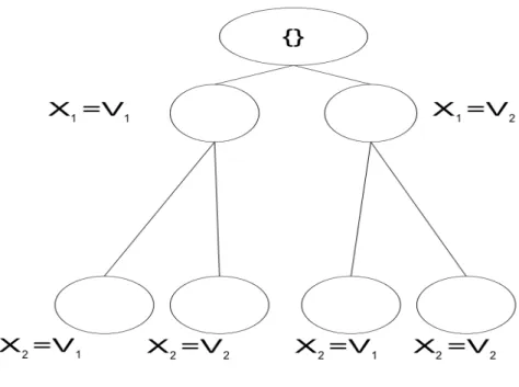
a value to each of the variables. Then we visualize the search as a tree. The root node is{}. The remaining nodes in the tree represent single assignments and the edges connect different single assignments. A path from the root to any node is a partial assignment. For example, Figure 2.1 shows a full search tree for two variables, in which x1 has two values, andx2 has two values. A

solution will be a path from the root down to one of the leaves whose values satisfy all constraints in this problem.

Generate and Test

Generate and Test (GT) generates an assignment in which each variable is assigned a value, and tests whether the assignment satisfies all of the constraints. If not, GT tries another assignment. Although GT can be implemented as a Depth First Search, it still has to traverse the whole search space in the worst case. GT is not efficient because the worst case time complexity is exponential in the number of variables. Therefore, GT is impractical except for very small problems.

(18)

Figure 2.1: An example of search tree including two variables

Backtracking

Instead of traversing the whole search space (i.e., the Cartesian product of all the variable do-mains), Backtracking (BT) prunes inconsistent partial assignments. Some partial assignments are inconsistent because they violate some constraints. If a partial assignment is inconsistent, it cannot be extended to a consistent assignment by assigning more values to the uninstantiated variables. BT uses this property to stop assigning values to variables following an inconsistent assignment. If there are more values to try in the current variable, BT tries to assign those values in some order. Otherwise, BT backtracks to the most recently assigned variable.

Because of thrashing, which means search in different parts of the space keeps failing for the same reasons (Kumar, 1992), BT’s performance is still exponential in the number of variables. One cause leading to thrashing is node inconsistency, in which a certain variable’s values do not satisfy a unary constraint on that variable, thus leading to an inconsistent assignment each time

(19)

BT tries to assign those values. More specifically, suppose variablexiis node inconsistent. In other words, a value vi ∈di violates the unary constraint on xi. Whenever BT tries to assign vi to xi, the assignment will violate the unary constraint on xi and the search backtracks to the previous variable. Therefore, the value assignment ofvi to xi keeps failing for the same reason.

Another cause of thrashing is that a value assigned to a variablexi in the ordering may conflict with all values of a variablexj which comes afterxi. For example, suppose the ordering of variable instantiation is x1,· · ·, xi,· · ·, xj,· · · , xn. For a value v ∈ di, if a constraint forbids any value

being assigned to xj wheneverv is assigned toxi, then each time after BT assigns v toxi, it will backtrack later when trying to assign any value toxj, thus leading to unnecessary assignments of values to vk, i < k < j. In general, BT does not remember inconsistencies it found in previous branches of the search tree because BT backtracks to the most recent variable, rather than to a variable that is responsible for the inconsistent assignment.

Backjumping, Backmarking, and the Hybrid of Backjumping and Backmarking

In order to prevent thrashing, three algorithms based on BT are developed by remembering the reasons for past backtrackings. Each algorithm avoids thrashing by either looking forward or looking back along the current partial assignment which can provide valuable information about possible reasons for thrashing.

The first method is Backjumping (BJ) (Prosser, 1993). When a partial assignment violates some constraints, BJ always jumps back to the culprit, which is the most recently instantiated predecessor found incompatible with any of the newly instantiated variable’s values. So, BJ avoids the unnecessary repetition of instantiation failures which will be encountered in BT. For example, suppose the variable ordering isx1,· · ·, xi,· · ·, xj,· · ·, xn. For a valuev∈di, if a constraint forbids

any value being assigned to xj wheneverv is assigned toxi, then each time BJ tries to assign any value to xj after v is assigned to xi, it will backtrack toxi, thus avoiding unnecessary repetitive assignment of values toxk, i < k < j.

(20)

BM avoids checking the constraints which have already been checked in an earlier instantiation. There are two types of unnecessary constraint checks. One is known to fail, and the other is known to succeed. In the case of unnecessary constraint checks that are known to fail, suppose we are instantiating a new valuev to the current variablexi. Then, we check the value assignmentxi=v

against all previous value assignments. Namely, we check xi =v againstx1 =a∈d1 first. If the

check succeeds, we continue to check x2 = b ∈ d2 and so on, until the check fails. Assume that

the constraint check betweenxh =g∈dh and xi =v fails (h < i), we can deduce from this point that: If the next time we are instantiating xi =v again and xh has not been re-instantiated to another value, then the constraint check between them will fail. So, there is no need to perform this constraint check and we can backtrack. In the case of unnecessary constraint checks that are known to succeed, suppose since last time we visited xi we have backtracked to xj (j < i), and we have re-instantiated all the variables fromxj to xi−1 again. Then we know that the constraint

checks between xk andxi are going to succeed, for allk < j. So, we can avoid those constraint checks and only check the constraints betweenxl andxi, for allj ≤l < i.

Experimental results showed that BM and BJ are more efficient than GT and BT on solving CSPs. Nadel (Nadel, 1989) suggested combining BM and BJ and Prosser (Prosser, 1993) imple-mented the hybrid BMJ algorithm. However, Prosser found that BMJ does not inherit all the power from BM and BJ. BMJ may even perform worse than BM “because the advantage of backmarking may be lost when jumping back” (Prosser, 1993).

2.2.2 Consistency Propagation

Consistency Propagation (CP) is another popular method for solving CSPs, because it removes inconsistent values from domains, thus reducing the search space. A binary constraint problem can be modelled as a constraint graphG= (V, E), whereV is a set of nodes, andE is a set of edges. Eachv∈V represents a variable and eache∈Erepresents a constraint between two variables. For constraint problems withk-ary constraints wherek >2, a hyper-graph can be used to represent it. The consistency can be classified into three levels: node-consistency, arc-consistency, and

(21)

k-consistency (k > 2). Node-consistency propagation prunes inconsistent values by checking the unary constraints. Arc-consistency propagation removes inconsistent values by checking binary constraints. K-consistency propagation removes values by checkingm-ary constraints (2≤m≤k). Usually, node-consistency and arc-consistency propagations cannot guarantee that a solution can be found without search in general. If an-node constraint graph isn-consistent, then a solution can be found without any backtracking. Unfortunately, the time complexity to enforce n-consistency in an-node constraint graph is exponential inn.

Node and Arc Consistency

The following definitions are based on concepts introduced by Mackworth (1977). They are the foundations of all the techniques we will discuss in this thesis.

Definition 2.5. Node Consistency . A value vi ∈ di is node consistent if it is permitted by the unary constraintci defined overxi. xi is node consistent if all of its values are node consistent. A CSP is node consistent if all of its variables are node consistent.

Definition 2.6. Arc Consistency . Suppose a binary constraint c ∈ C is represented by an arc (xi, xj) in the constraint graph. The constraint is arc consistent relative to xj if for every value

v ∈ di, there is some value w ∈ dj such that the value combination (v, w) is permitted by the constraint c. Valuew is called a support for the valuev.

To make a variable node consistent, all values violating the unary constraint of the variable have to be deleted. To make a binary constraintcij arc consistent relative toxj, all values fromdi

which do not have any support indj have to be deleted.

Waltz (Waltz, 1975) initiated the research on constraint propagation algorithms by introducing an algorithm for three-dimensional cubic drawing interpretations. His empirical results demon-strated that for some polyhedral problems, basic arc consistency algorithms are able to solve them. The basic operation is REV ISE (Mackworth, 1977) which prunes values from di to make the constraintcij arc consistent relative to xj. To make a CSP arc consistent, it is not sufficient to perform REV ISE on each constraint just once, because the pruning of values may make some

(22)

arc consistent constraints inconsistent, if the pruned values are the only supporting values for some other domain’s remaining values. AC1 (Mackworth, 1977) is a simple intuitive algorithm for consis-tency propagation. It repeatsREV ISEon each arc until no domains are changed or some domain becomes empty. AC1 is not efficient because it checks all the arcs again even if only one arc is changed. AC3 (Mackworth, 1977) improves AC1 by maintaining a queue of constraints waiting to be processed, thus checking only the constraints for variables whose supports may have changed. Other versions of consistency propagation include AC2 (Mackworth, 1977) which is a special case of AC3, AC4 (Mohr and Henderson, 1986) which builds additional data structures to simplify the propagation process, and so on.

Arc consistency (AC) can be interpreted as an operation transforming a problem into an equiv-alent one, possibly with some domain values removed, in order to reduce the search space. When using AC for preprocessing before the search starts, if some domains become empty, then there is no solution. However, AC does not completely eliminate the need for search. If there is no empty domain and at least one domain has more than one value after AC is done, we still have to search the remaining constraint graph to find a solution.

A powerful hybrid way to solve CSPs is to combine consistency propagation (CP) and search, in which AC propagation is performed at each new value instantiation during the search. When a value is assigned to a variable, the domain of this variable is reduced to contain only this value. Then AC propagation removes values without support. For example, suppose the variable ordering is{x1,· · ·, xi,· · ·, xn}, and variablesx1,· · ·, xi have already been assigned values. When a value

v∈di+1 is assigned toxi+1, AC propagates over the constraints in the constraint graph to delete

values without support. If AC propagation leads to empty domains, the search procedure will try to assign another value toxi+1 or backtrack toxi if there is no more value available in xi+1.

Although AC propagation can reduce the search space substantially, it requires more constraint checks than exhaustive search during each new value instantiation. There is a trade-off between the AC propagation and the search.

(23)

2.2.3 Heuristics

A heuristic is a procedure that guesses the best option based on information available during problem-solving: Instead of pursuing a definite correct answer, a heuristic tries to find a good enough approximation to the best answer. Heuristics are designed to increase computational performance, probably at the cost of accuracy or precision. Due to the efficiency of heuristics, they are used in many real world applications. For example, some medical expert systems use heuristics to deduce approximate diagnoses of a disease.

In tree search, a heuristic is used to choose variables and instantiate values. Instead of choosing the globally best variable or value at each instantiation point, which is expensive, a good enough heuristic is a relatively inexpensive procedure that tries to guide the search to the answer as fast as possible. For solving CSPs, there are two typical uses of heuristics, namely variable ordering and value ordering.

A variable-ordering heuristic re-orders the variables for instantiation in tree search, instead of using an arbitrary ordering (see Page 31). For example, the algorithmsearch rearrangementalways chooses a variable with the least number of values remaining as the next instantiation, hoping to force backtracks to happen as early as possible (Bitner and Reingold, 1975). Compared with a lexicographical ordering, this method may traverse fewer nodes because a backtrack is likely to be triggered earlier in the search. However, this method can be ineffective in some cases, especially at the beginning of the search, where all the variables have the same remaining domain size. In order to avoid this pitfall, a static ordering is introduced which chooses a variable with the minimum remaining domain values and breaks ties by choosing the variable which has the largest number of constraints connected to future variables in the search tree (Br´elaz, 1979). If multiple variables have the same remaining domain size and constrain the same number of future variables, additional tie breakers will break the ties by the domain size of the smallest neighbour and the number of triangles in which the first chosen variable is involved (Smith, 1999). Another famous variable ordering iscycle-cutset decomposition (Dechter, 1990). Since a tree-structured CSP can be solved in linear time without backtracking once it is node and arc consistent (Kumar, 1992), the

(24)

cycle-cutset heuristic tries to find a small set of variables whose removal makes the constraint graph tree-structured, and orders those variables earlier in the search tree than other variables. A variable can be removed from the constraint graph by assigning a value to it. However, finding the smallest cutset is NP-hard, so the cycle cutset decomposition is incorporated into tree search by instantiating variables unchanged after enforcing consistency, and triggering a specialized tree-solving algorithm on the remaining graph once a tree structure is encountered (Dechter, 1990). This method is not guaranteed to find a minimum cycle cutset, but it is a fast heuristic that is able to find a good approximation. If the constraint graph is complete, then the cycle cutset decomposition reverts to naive backtracking.

A value-ordering heuristic re-orders the values to be assigned to the next variable. For example, the value-ordering heuristic introduced by Dechter and Pearl (1988) approximates the number of possible solutions in the subtree associated with each value of the current variable and chooses the value with the highest number to instantiate the next variable. Vernooy and Havens (1999) introduced another dynamic value-ordering heuristic which decomposes a CSP into a disjoint set of spanning trees and uses Bayesian networks to approximate solution probabilities for different values based on the current search state. xAC (Section 3.3) can be treated as a dynamic value ordering heuristic for COPs.

2.2.4 Local Search

Local search algorithms start with a random initial full assignment. These algorithms then explore other full assignments most of whose values are the same with the initial assignment except for a few. These full assignments are called a local neighbourhood. From this local neighbourhood, a best assignment which maximizes the number of satisfied constraints is selected. Then these local search algorithms restart the neighbourhood exploration procedure to find a better assignment until a local maximum (i.e., the best assignment does not change after restart) is reached. Since a local maximum is not guaranteed to be the global maximum, the local search algorithms either restart from another random full assignment or considers other locally sub-optimal assignments as well as

(25)

the locally optimal one (Selmanet al., 1992).

Compared with tree search and consistency propagation, local search is incomplete because it cannot guarantee to find a solution or prove there is no solution. Empirical analysis has shown that the performance of local search is strongly influenced by the number of solutions and problem hardness. For local search algorithms, the hardest CSPs usually have few solutions and occur during the solubility phase transition (Clarket al., 1996). Generally speaking, a CSP is considered easy to solve if there are too many solutions or the problem is highly over-constrained. On the other hand, it is considered hard to solve when the number solutions is close to one.

2.2.5 Summary of CSP Algorithms

Section 2.2 reviewed tree search and AC propagation for solving CSPs, examined the hardness of CSPs and empirical evaluation of different algorithms, and discussed several variable and value ordering heuristics.

Tree search algorithms are complete, but inefficient. A simple backtracking algorithm does not learn from the failure of different nodes, thus leading to repetitive instantiations of the same set of variables. Therefore, AC propagation is performed at each node of the search tree to reduce the search space, thus improving the performance. Other techniques to improve the efficiency of tree search include learning the reason for failure and choosing the right variable or value ordering. Similar to CSPs, many algorithms for solving COPs adopt and modify successful CSP algorithms. The following sections introduce the work in COP and focus on the soft arc consistency algorithms (see Chapter 3).

2.3 Constraint Optimization Problems

Although many real world problems are perfect CSP instances, some of the problems require us to find an assignment of values to variables that has an optimal value, either maximum or minimum. In order to solve these problems, several extensions of the CSP framework were proposed by tak-ing into account priorities (Schiex, 1992; Borntak-inget al., 1989), costs (Shapiro and Haralick, 1981),

(26)

uncertainties (Rosenfeldet al., 1976), preferences (Rosenfeldet al., 1976), etc. These frameworks address problems which are called Constraint Optimization Problems (COPs).

2.3.1 Hard and Soft Constraints

A classical CSP either allows a tuple in a constraint or forbids it, with no choice of expressing degrees of satisfaction. In a real world problem, however, we need to represent various levels of satisfaction, such as degrees of preference, or costs. Constraints can be categorized into three groups (Schiexet al., 1995):

• “Hard” constraints: properties which have to be satisfied in all cases, e.g., physical properties;

• Preferences: properties which should be satisfied;

• Uncertainties: properties that are relevant in some situations which cannot be predicted with certainty; such properties may be ignored or represented as constraints.

The “soft” constraints include the second and third groups. In order to utilize “soft” constraints, a new methodology is introduced to transfer the violation of these “soft” constraints into aspecific criterionthat should be minimized (Schiexet al., 1995). In the following sections, we will review the concepts of VCSPs, SCSPs, and WCSPs, which are the mathematical models for “soft” constraints.

2.3.2 Valued Constraint Satisfaction Problems

Due to various formulations of “soft” constraints, each of which uses its own operators and interpre-tation of the violation of constraints, an ordered commutative monoid is introduced to encompass most “soft” CSP extensions (Schiexet al., 1995). A monoid is an algebraic structure with a single associative binary operation and an identity element. For example, the natural numbers form a commutative monoid with addition as the commutative binary operation and zero as its identity element (the integers also form a monoid with multiplication as the binary operation, and one as its identity element).

(27)

is a set of finite domains each of which corresponds to a variable, andCis a set of constraints each of which forbids certain value combinations of the variables involved in the constraint. A constraint can also be viewed as a pair ci =hsi, rii, where si is called the scope of ci, andri is a relation defined on si. The scope si includes the variables affected by ci. Suppose si = {xi1,· · · , xir}, then ri ⊆ di1× · · · ×dir. A solution is an assignment of values to all the variables satisfying all constraints.

To express “soft” constraints, instead of allowing absolute satisfaction or violation, valuation is used to generalize the degree of preference or cost. Tuples in a constraint are associated with elements taken from a valuation structure:

Definition 2.7. (Schiexet al., 1995) A valuation structureS=hE,⊛, >iconsists of:

• E is a set, whose elements are called valuations, which are totally ordered by >, with a maximum element ⊤and a minimum element⊥;

• ⊛_{is a commutative, associative closed binary operation on} _E_:

– Identity: ∀a∈E, a⊛⊥=a;

– Monotonicity: ∀a, b, c∈E,(a≥b)⇒((a⊛_c₎≥₍_b⊛_c_));

– Absorbing element: ∀a∈E,(a⊛⊤) =⊤.

Definition 2.8. (Schiex et al., 1995) Strict monotonicity. ∀a, b, c ∈E, if (a > c),(b 6=⊤), then (a⊛_b₎_>₍_c⊛_b_).

Strict monotonicity is very useful since the quality of a potential solution is determined by combining valuations of the assignments associated with that solution. However, strict monotonicity is too restrictive for certain classes of COPs.

Definition 2.9. (Schiexet al., 1995) A binary operation⊛is idempotent if∀a∈E, a⊛a=a. Idempotency is incompatible with strict monotonicity once Ehas more than two elements. To see this, we have∀a∈E, a⊛⊥=a, according to identity. Therefore,∀a∈Esuch that⊥< a <⊤,

(28)

strict monotonicity implies that (⊥⊛a)<(a⊛a), which implies thata <(a⊛a). Clearly,a <(a⊛a) means that the binary operation⊛_{is not idempotent.}

Based on Definition 2.7, a valued CSP is defined as follows.

Definition 2.10. (Schiex et al., 1995) A Valued CSP (VCSP) is defined by a classical CSP(X, D, C), a valuation structureS =hE,⊛_{, >}_i_{, and a function}_φ_from_C_to_E_{. A VCSP is denoted}₍_{X, D, C, S, φ}_), andφ(c)is called the valuation of c.

The valuation of an assignment is a combination of valuations of involved constraints, each of whose scopes is a subset of the variables inX. The combination is calculated using⊛.

Definition 2.11. (Schiexet al., 1995) Given a VCSPP= (X, D, C, S, φ)and a partial assignment

A of the variablesY ⊂X, the valuation or cost ofA with respect toP is defined by:

VP(A) = ⊛

c∈C,A violates c[φ(c)]

In Definition 2.11, the valuation of a partial assignment is the combination of the valuations of all the constraints which violate the partial assignment. This valuation of partial assignment can be interpreted as the cost or preference of the partial assignment.

The valuations in E represent degrees of inconsistency or consistency. Usually, the valuation of an assignment is interpreted as the level of inconsistency; the higher the valuation, the worse the assignment. Therefore, a COP can be solved by finding an assignment A with a minimum valuation, such that VP(A) ≤ VP(B), for all possible assignments B. Notice that ⊥ represents

complete consistency and⊤complete inconsistency, thus a lower valuation is preferred to a higher one.

2.3.3 Semiring-Based Constraint Satisfaction Problems

A Semiring-Based CSP (SCSP) is another framework subsuming all “soft” extensions of classical CSPs in order to model COPs (Bistarelliet al., 1999). A SCSP is based on a semiring structure (see Definition 2.12), which consists of a set of valuations plus two operators. More specifically, these valuations describe degrees of consistency which can be interpreted as preferences or costs.

(29)

There are two operators which define how to combine constraints in order to generate a combined valuation or preference level.

The original definition of SCSPs (Bistarelliet al., 1999) specified two extreme elements: 0 rep-resents the worst or the least preferred choice and 1 represents the best or the most preferred choice. Since the valuation structure in VCSPs is a specific semiring, we use⊤, the worst element in VCSP, to represent 0;⊥, the best element in VCSP, to represent 1. We modified the original definitions (Bistarelliet al., 1999). Our definitions are as follows.

Definition 2.12. A semiring is a tuple(A,+,×,⊤,⊥)such that

• A is a set;

• there are two extreme elements in A: ⊤ and ⊥, where ⊤ represents the worst or the least preferred choice and ⊥represents the best or the most preferred choice;

• +is the additive operation, which is a closed (i.e., a, b∈A impliesa+b∈A), commutative (i.e., a+b = b+a), and associative (i.e., a+ (b+c) = (a+b) +c) operation such that

a+⊤=a=⊤+a, where⊤is the unit element of+;

• × is the multiplicative operation, which is a closed and associative operation such that ⊥is its unit element and a× ⊤=⊤=⊤ ×a. ⊤is the absorbing element;

• ×distributes over +, i.e., a×(b+c) = (a×b) + (a×c).

Definition 2.13. A c-semiring is a semiring such that + is idempotent (i.e., a ∈ A implies

a+a=a),×is commutative, and⊥is the absorbing element of +.

Since + and × are generic operators, we can assign any semantics to them. However, there are some common requirements for these operators, no matter what the actual semantics are. For example, + is used to define a partial ordering≤S: a≤S bif and only ifa+b=b. a≤S b means

b is at least as good as a. Notice that the idempotency of + is necessary to define ≤S, because a≤S a if and only ifa+a= a. Using the partial ordering≤S, we can define the best solution.

Notice that both + and × are monotonic on ≤S, i.e., a ≤S b, c ∈ A and c is not an absorbing

(30)

In a c-semiring, ⊥is the absorbing element of the additive operation, i.e., a+⊥=⊥, which implies ∀a, a ≤S ⊥. Therefore ⊥ is the maximum or the best element inA. Similarly, ⊤ is the

minimum or worst element of the ordering ≤S because ∀a, ⊤+a = a implies that ⊤ ≤S a.

Therefore, ∀a ∈ A, we have ⊤ ≤S a ≤S ⊥. According to the monotonic property of × over A, b≤S ⊥impliesb×a≤S⊥ ×awhich impliesa×b≤S a. So, the×operation isextensive, because a×b≤S a. Intuitively, combining two valuations always results in one that is no better than either

of them.

In the following sections,×may be closed on a certain finite subset of the c-semiring.

Definition 2.14. Given any c-semiring S = (A,+,×,⊤,⊥), and a finite set I ∈A. × is closed on I; if ∀a, b∈I,a×b∈I.

In order to incorporate a semiring into the framework of CSPs, constraint systems are introduced (Bistarelliet al., 1999). A constraint system includes a c-semiring, a set of variables, and a set of domains corresponding to these variables. A constraint associates an element in the c-semiring to a tuple in the constraint relation. Similar to a valuation in a valuation structure in VCSPs, this element in a c-semiring can be interpreted as a cost or a preference. A constraint problem consists of a constraint system and a set of constraints, plus a selected set of variables. Notice that this set of variables may not be the set of all variables, because we may want to assign values to a subset of all variables.

Definition 2.15. (Bistarelli et al., 1999) A constraint system is a tuple CS = hS, D, Vi, where

S is a c-semiring, D is a finite set, and V is an ordered set of variables. Given a constraint systemCS=hS, D, Vi, whereS= (A,+,×,⊤,⊥), a constraint overCS is a pairhdef,coni, where con⊂V anddef :dk _→_A _where_k _{is the size of}_con_{or the number of variables in it.} _con_{is called}

the type of the constraint, and def is called the value of the constraint. Moreover, a constraint problem P overCS is a pair P =hC,coni, where C is a set of constraints overCS andcon⊂V. If ×is not idempotent, thenC becomes a multi-set.

(31)

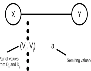
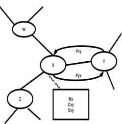
is a graphical representation of a constraint. In a graphical representation, a variable is a node and a constraint is an arc. Domains and constraints are labels of the corresponding graphical objects.

Figure 2.2: Structure of a Constraint

The following discussion uses a constraint system CS =hS, D, Vi, where S = (A,+,×,⊤,⊥). A special set of variables includes the variables of every constraint: V(P) =∪_hdef_,_con′_i∈

Ccon ′ . Since the elements inAare associated with tuples of constraints, an SCSP’s constraints can be manipulated by ×and +. More specifically, two operations,combination ⊗and projection ⇓, are defined using×and +.

Definition 2.16. For any tuple t= (t1, t2,· · ·, tn)in the cartesian product of domain values in a

variable set I, given another variable set I′, the projection of t over the variables in the setI′ is defined as t↓I I′= (t ′ 1, t ′ 2,· · · , t ′

m), such that anyt ′ i is a domain value ofd ′ i, wherex ′ i∈I ′ ∩I.

Definition 2.17. (Bistarelliet al., 1999) Consider two constraints c1 = hdef1,con1i and c2 =

(32)

anddef(t) = def(t↓con

con1)×def(t↓

con

con2), where, for any tupletin a setI,t↓ I

I′ denotes the projection of t over the variables in the setI′. Moreover, given a constraint c =hdef,coni over CS, and a subset w of con, its projection over w,c ⇓w, is the constraint hdef

′

,con′iover CS withcon′ = w anddef′(t′) =P

{t|t↓con

w =t′}def(t).

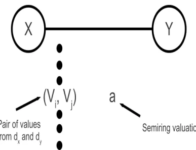
Figure 2.3 shows an example of combination and projection. A solution of an SCSP can now be defined using these two operations.

Figure 2.3: An Example of Combination and Projection

Definition 2.18. (Bistarelliet al., 1999) Given a constraint problem P = hC, coni over a con-straint system CS, the solution of P is a constraint defined as Sol(P) = (N_C₎ _⇓

con, where

N_C₌_c

1⊗c2⊗ · · · ⊗cn, C ={c1, c2,· · ·, cn}. The entity including the constraint problem P and

the constraint system CS is called an SCSP.

In other words, the solution of an SCSP is an induced global constraint which combines all constraints in the problem and associates valuations inAto each tuple of values ofD. Notice that

(33)

Definition 2.18 specifies the semantic of the solution of a problem, not how to solve it.

2.3.4 Comparison of SCSPs and VCSPs

Given a variable ordering, it is possible to transform any SCSP into an equivalent VCSP, and vice-versa (Bistarelliet al., 1999). These transformations are explained in the following sections.

From SCSPs to VCSPs

An SCSPhC, coniwhereconinvolves all variables is considered in the following sections. Recalling the definition of SCSP, it is a set of constraintsC over a constraint system hS, D, Vi, whereS = (A,+,×,⊤,⊥) is a c-semiring,Dis a set of domains, each of which corresponds to a variable inV. For this section, assumptions are made that + induces a total ordering≤S, which indicates that +

corresponds to an operator that always chooses a valuation closer to⊥among any two valuations because⊥means total consistency (Bistarelliet al., 1999).

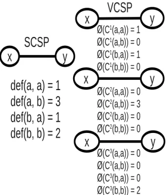
Given an SCSP, an equivalent VCSP assigns the same valuations to tuples, and has the same solutions (Bistarelliet al., 1999). For example, Figure 2.4 shows an SCSP which contains a con-straint c = hcon, defi, where con = {x, y}, and def(ha, ai) = 1, def(ha, bi) = 3, def(hb, ai) = 1, def(hb, bi) = 2. Then, the equivalent VCSP will contain three constraints, all of which constrain

xandy:

• c1, withφ(c1) = 1 and allowed tuplesha, biandhb, bi.

• c2, withφ(c2) = 3 and allowed tuplesha, ai,hb, ai, andhb, bi.

• c3, withφ(c3) = 2 and allowed tuplesha, ai,ha, bi, andhb, ai.

No matter how an SCSP is constructed, there is always an equivalent VCSP. In our experimen-tations (see Chapter 4, Chapter 5, and Chapter 6), xAC solves SCSPs, while W-AC*2001, EDAC, and VAC solve VCSPs.

(34)

Figure 2.4: From SCSP to VCSP

From VCSPs to SCSPs

In this section, we translate a VCSP to an equivalent SCSP (Bistarelliet al., 1999). For example, Figure 2.5 shows a VCSP with ⊥= 0,⊤ =M, where M is a finite integer, and ≥S is given the

semantics of≤over integers. This VCSP contains a binary constraintc between variablesx and

y. The constraintc allows tuplesha, aiandhb, bi, and such thatφ(c) = 1. Then the corresponding SCSP will contain the constraint c′ =hcon, defi, where con={x, y}, def(ha, ai) =def(hb, bi) =

⊥= 0, anddef(ha, bi) =def(hb, ai) = 1. Notice we assume a cost of 0 equals⊥.

If there are multiple VCSP constraints defined over the same subset of variables, each of the constraints can be converted into an SCSP constraint and all of the SCSP constraints can be combined using the multiplicative operator (see Definition 2.12). For example, each of the VCSP constraints on the right hand side in Figure 2.4 can be converted into an SCSP constraint and the resulting SCSP constraints can be combined (i.e., all the costs of each tuple are sumed) to form

(35)

Figure 2.5: From VCSP to SCSP

the SCSP constraint on the left hand side.

2.3.5 Weighted CSPs

Both VCSP and SCSP can be used to model Weighted CSP (WCSP), which is another one of the main frameworks for COPs (Bistarelliet al., 1999).

VCSP Model for WCSP

A Weighted CSP (WCSP) assigns weights or degrees of preferences to the tuples in constraints. These weights represent the costs of violating the constraints. Solving WCSPs means minimizing the weighted sum of the elementary weights associated with violated constraints among all potential solutions. VCSP models WCSP by giving the operation⊛_{the semantic of arithmetic addition on} integers. The set E in the valuation structure S contains natural numbers plus positive infinity, which is N ∪ {+∞}. The ordering over E is the usual binary operator <over natural numbers.

(36)

Notice that⊛is strictly monotonic.

SCSP Model for WCSP

In SCSP, a WCSP can be modelled as an SCSP with a c-semiringS_{W CSP}− =hR−_{, max,}₊_,_−∞_,₀_i_,

where ordering ≤S is given the semantics of ≤ over real numbers. Or, the c-semiring can be S_{W CSP}+ =hR+_{, min,}₊_,₊_∞_,₀_i_{, where ordering}_≤

S equals ≥over real numbers. Notice that the

former c-semiring represents costs as negative numbers and the latter represents them as positive numbers.

If a WCSP problem has a best solution with costα, then the best solution of any subproblem has a cost that is at leastα. Therefore, we can use the cost of the best solution found so far as the upper bound in a branch and bound search. If the current partial solution’s cost is greater than α, we can prune the current branch. Notice that the same properties hold for the semirings over rational costs and integer costs: hQ−_{, max,}₊_,_−∞_,₀_i_and_hZ−_{, max,}₊_,_−∞_,₀_i_(Bistarelli_{et al., 1999).}

2.4 Summary

In this chapter, we reviewed the current frameworks for constraint satisfaction problems and con-straint optimization problems. We demonstrated how Valued CSPs and Semiring CSPs are derived from classical CSPs and how to transform each one into an equivalent other. This chapter builds the theoretical foundation for the following chapters.

(37)

Chapter 3 Soft AC Algorithms

In this chapter, we briefly review algorithms W-AC*2001, EDAC, VAC, and xAC, all of which can be used to solve general COPs. W-AC*2001, EDAC, and VAC solve WCSPs modelled by VCSPs, while xAC solves WCSPs modelled by SCSPs. Since we have shown that both VCSPs and SCSPs can be used to model WCSPs in Section 2.3.5, we can model the same WCSPs with VCSPs or SCSPs, which produce the same solutions. We note that VAC is state-of-the-art for solving COPs (Cooperet al., 2008). We use AC* to refer to W-AC*2001 in this chapter in order to show the connection between AC*, FDAC*, and EDAC*.

3.1 Preliminary

3.1.1 Conventions

In the literature, it is common for authors to use an acronym in two ways: one as an algorithm, the other as a property realized after the algorithm is applied. In this thesis, AC* refers to the algorithm W-AC*2001 or the arc consistent property W-AC*2001, depending on context.

3.1.2 Arc Consistency Closure

Definition 3.1. (Robert, 1999) A set of objects,O, is said to exhibit closure or to be closed under a given operation,R, provided that for every object, x, ifxis a member ofO andxisR-related to any object, y, theny is a member ofO.

For example, real numbers are closed under the subtraction operation because the result of performing subtraction among any pair of real numbers is a real number. But natural numbers

(38)

are not closed under the subtraction operation because the result of performing subtraction among some pairs of natural numbers may be negative, which is not a natural number.

By applying Definition 3.1 to classical arc consistency (Mackworth, 1977), we get the following definition of arc consistency closure.

Definition 3.2. Given a set of objectsOwhich is a set of constraints, a given operationRwhich is theREV ISEoperation (Mackworth, 1977), and every objectxwhich is an arc consistent constraint in O, a CSP is an arc consistency closure if the result of applying R (i.e., REV ISE) to x is a constraint y that is arc consistent.

In other words, an arc consistency closure is a CSP whose domain values and solutions will not change no matter how many times theR operation (i.e., theREV ISEoperation in the context of classical CSPs) is applied. An arc consistency closure is closed under the operationREV ISE.

Although applying theREV ISEoperation multiple times in a classical CSP can reach a unique arc consistency closure (see Section 2.2.2), applying soft arc consistency operations (described in this chapter) is not guaranteed to reach a unique soft arc consistency closure. Therefore, peo-ple continue to research algorithms to produce better closures that can improve the efficiency of problem solving (Schiex, 2000; Larrosa, 2002; Cooper and Schiex, 2004; Givry and Zytnicki, 2005; Cooperet al., 2008).

3.2 W-AC*2001 and EDAC

3.2.1 Foundation

Based on the notation of VCSP, a single axiom is introduced to define an extended arc consistency (AC) which has all the properties of a classical arc consistency except for the uniqueness of the arc consistency closure (Cooper and Schiex, 2004). An arc consistency closure is a COP obtained by removing all arc inconsistent values from the problem’s domains. If the VCSP binary operation + is idempotent, then the new AC closure reduces to classical definitions and uniqueness is recovered. The new axiom added to the VCSP framework is based on an intuition that we can transfer a

(39)

VCSP into an equivalent one by shifting costs of constraints. The idea can be formalized, starting with the definition of a difference of two valuations:

Definition 3.3. (Cooper and Schiex, 2004) In a valuation structureS =hE,⊕,i, if α, β ∈E,

αβ, and there exists a valuation γ∈E such that α⊕γ=β, thenγ is known as a difference of

β andα. αβ is equivalent toβ α.

Definition 3.4. (Cooper and Schiex, 2004) The valuation structureS is fair if for any pair of valuations α, β ∈ E, with α β, there exists a maximal difference of β and α. This maximal difference of β andαis denoted byβ⊖α.

Theorem 3.1. (Cooper and Schiex, 2004) Let S =hE,⊕,i be a fair valuation structure. Then

∀u, v, w∈E,wv, we have(v⊖w)v and(u⊕w)⊕(v⊖w) = (u⊕v).

Most existing soft constraint frameworks are fair. For example, in order to count costs as integer values, we can define a strictly monotonic valuation structure hN ∪ {∞},+,≥i. β⊖α =β−α

for finite valuations α, β ∈ N, α ≤β and (∞ ⊖α) = ∞ for allα∈ N ∪ {∞}. Although ⊖may not exist in general cases of any strictly monotonic operator ⊕, it can always be constructed by deriving a larger valuation structureE×E, where each valuation (β, α) represents the imaginary

β⊖α(Cooper and Schiex, 2004). This is similar to extending real numbersRto complex numbers

C in order to represent square roots of negative numbers.

Equivalence Preserving Transformations

Definition 3.5. A value assignment is a tuple(i, a)which denotes assigning valuea∈dito variable

xi∈X. (In Chapter 2, we used a different notation for this.)

Definition 3.6. (Cooper and Schiex, 2004) The subproblem of a VCSPV =hX, D, C, SionJ ⊂X

is a VCSPV(J) =hJ, DJ, CJ, Si, whereDJ={dj :j∈J} andCJ ={cP ∈C:P ⊂J}.

Definition 3.7. (Cooper and Schiex, 2004) For a VCSPV, an equivalence-preserving transforma-tion ofV onJ ⊂X is an operation which transforms the subproblem ofV onJ into an equivalent

(40)

V CSP, which has the same J and solutions. If CJ ={cP ∈ C : P ⊂J} contains only one non unary constraint, such an operation is called an equivalence-preserving arc transformation.

Procedures 1 and 2 show two operations Project and Extend that transform a VCSP into an equivalence. For a subproblem V(J) = hJ, DJ, CJ, Si, l(J) denotes the set of all possible value assignments forJ (i.e., the Cartesian product of alldi∈DJ). Procedure 1 projects the minimum cost in a given non-unary constraintcP down to a valuea∈di, wherei∈P, a∈di. The procedure adds the minimum cost to the unary constraint of ci and subtracts that cost from the non-unary constraintcP in order to preserve equivalence. Conversely, Procedure 2 extends the cost from value

a∈ di to the non-unary constraint cP by subtracting the cost ci(a) from the unary constraintci

and adding that cost to the non-unary constraintcP.

Procedure 1 Project(cP, i, a)

Input: a variablei, a valuea∈di, and a constraintcP β←mint∈l(P−{i})(cP(t, a)) ci(a)←ci(a)⊕β foreacht∈l(P− {i})do cP(t, a)←cP(t, a)⊖β end for Procedure 2 Extend(i, a, cP)

Input: a variablei, a valuea∈di, and a constraintcP

for allt∈l(P− {i})do

cP(t, a)←cP(t, a)⊕ci(a)

end for

ci(a)←ci(a)⊖ci(a)

3.2.2 W-AC*2001 and Directional Arc Consistency

The Weighted Arc Consistency 2001 (W-AC*2001) (Larrosa, 2002) and the Full Directional Arc Consistency (FDAC*) refine the original soft AC (Schiex, 2000) to provide better guidance for a branch-and-bound search. The W-AC*2001 algorithm and the FDAC* algorithm are based on the VCSP framework introduced in Section 2.3.2.

(41)

Local Consistency in WCSP

In this section we review the definitions of consistency as applied to variables and constraints (Larrosa, 2002; Larrosa and Schiex, 2003). We assume the variable set X is lexicographically or-dered according to a sequence given by the problem statement.

Definition 3.8. LetP = (X, D, C, S, φ)be a binary WCSP, whereX is a set of variables, D is a set of domains, C is a set of constraints,S= (N ∪ {+∞},+, >)is a valuation structure, andφis a function mapping a constraint tuple to a valuation inS. The maximum cost is denoted by⊤and the minimum cost is denoted by ⊥.

• Zero-arity Constraint: c∅ is the zero-arity constraint which is usually the lower bound for a

branch-and-bound search. This constraint’s value indicates the least amount of cost for the optimal solution at any given point in the search.

• Node consistency (N C∗_{): The value assignment}₍_{i, a}₎_{is node consistent (}_{N C}∗_{) if}_c

∅⊕ci(a)<

⊤. Variable i isN C∗ _{if: 1) all its values are} _{N C}∗_{, and 2) there exists a value} _a_∈_di _such

that ci(a) =⊥. Valueais a support for the variable i. P isN C∗ _{if every variable is}_{N C}∗_.

• Arc consistency (AC): The value assignment (i, a) is arc consistent (AC) with respect to constraint cij if there is a value b ∈dj such that cij(a, b) = ⊥. Value b is called a support of value a. Variable i is AC if all its values are AC with respect to every binary constraint affectingi. P isAC∗ _{if every variable is}_AC _and_{N C}∗_.

• Directional arc consistency (DAC∗_{): Given a variable ordering such that} _{i < j} _if _i _appears

earlier in the ordering thanj, the value assignment(i, a)is directional arc consistent (DAC∗₎

with respect to constraintcij, wherej > i, if there is a valueb∈dj such thatcij(a, b)⊕cj(b) =

⊥. Value b is called a full support of a. Variable i is DAC if all its values are DAC with respect to every cij, j > i. P isDAC∗ _{if every variable is}_DAC _and_{N C}∗_.

• Full Directional Arc Consistency (F DAC∗). P is fully directional arc consistent if it isDAC∗

(42)

Figure 3.1: A WCSP instance that is notN C∗

For example, Figure 3.1 is a constraint graph which shows a WCSP with ⊤ = 4,⊥= 0. In a constraint graph, small circles representing domain values are contained in larger circles which represent variables. Constraints are represented by edges showing non-zero cost tuples as labels. If there is no edge between two domain values, then there is zero cost associated with the tuple. Figure 3.1 is not N C∗ _{because variable} _x_{does not have a value} _a _{such that}_cx₍_a_{) =}_⊥_{. We can}

make this WCSPN C∗ by projecting a unary cost of one fromxdown toc∅. This unary projection

subtracts one cost from all values ofxand adds one cost to c∅. The result is Figure 3.2.

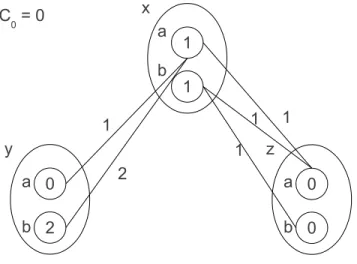
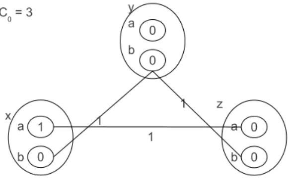
Figure 3.2 is not DAC∗ _{with respect to variable ordering} _xyz _{because the value} _a _of _x _has

no full supports in y, and the value b of xhas no full supports in z. We can make it DAC∗ _by

projecting a binary cost of one fromcxy down tocx and fromcxzdown tocx. Then we project the a cost of one from cx down toc∅. The binary projections from cxy to cx and cxz to cx shift one

cost from those binary constraints down to each value ofxand the unary projection fromcxtoc∅

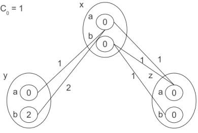
moves that one cost down to the zero-arity constraint. The result is shown in Figure 3.3. It can be shown that Figure 3.3 is alsoAC∗_{. Therefore, Figure 3.3 is}_{F DAC}∗_.

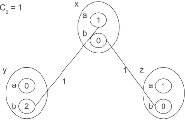
In Figure 3.3, a WCSP is madeAC∗ _{by making it} _DAC∗_{. However, if we choose to make the}

previous WCSP (Figure 3.2)AC∗by projecting binary costs fromcxy tocxandcxztocz, then the result is shown in Figure 3.4. It is notDAC∗ _{because (}_{x, b}_{) doest not have a full support in}_z_.

(43)

Figure 3.2: A WCSP instance that isN C∗

(44)

Figure 3.4: A WCSP instance that isAC∗ but notDAC∗

In WCSP instances, a support is not necessarily a full support. DAC∗ _{requires full supports}

on the variables later in the ordering while AC∗ _{requires a support on both variables.} _{F DAC}∗_,

which requires a support on one side and a full support on the other, is at least as strong asAC∗

or DAC∗_{. This property implies that the} _c

∅ ofF DAC∗ is equal to or stronger than that of AC∗

orDAC∗_{. In fact,}_{F DAC}∗ _{is stronger in many cases. One case is shown in Figure 3.3 and Figure}

3.4 which demonstrate thatF DAC∗ can produce a higher zero-arity constraint thanAC∗.

3.2.3 Enforcing Arc Consistency

In the previous section, we showed an example of how to achieve N C∗_{, AC}∗_{, DAC}∗_{, F DAC}∗ _by

shifting costs in the problem. In this section, we present algorithms to enforce these arc consisten-cies.

Let P = (X, D, C, S, φ) be a WCSP with a valuation structure S = ([0,· · · , k],+, >), where 0 represents the lowest cost or the most preferable valuation andk represents the worst cost or the least preferable valuation. We use + to combine costs or preferences and>to compare them. Let

Empirical evaluation of Soft Arc Consistency algorithms for solving Constraint Optimization Problems