Practical Enhancements in Sequential Quadratic Optimization: Infeasibility Detection, Subproblem Solvers, and Penalty Parameter Updates

(1)

Lehigh University

Lehigh Preserve

Theses and Dissertations

2015

Practical Enhancements in Sequential Quadratic

Optimization: Infeasibility Detection, Subproblem

Solvers, and Penalty Parameter Updates

Hao Wang

Lehigh University

Follow this and additional works at:

http://preserve.lehigh.edu/etd

Part of the

Industrial Engineering Commons

This Dissertation is brought to you for free and open access by Lehigh Preserve. It has been accepted for inclusion in Theses and Dissertations by an authorized administrator of Lehigh Preserve. For more information, please [email protected].

Recommended Citation

Wang, Hao, "Practical Enhancements in Sequential Quadratic Optimization: Infeasibility Detection, Subproblem Solvers, and Penalty Parameter Updates" (2015).Theses and Dissertations. 2862.

(2)

Practical Enhancements in Sequential Quadratic

Optimization: Infeasibility Detection, Subproblem Solvers,

and Penalty Parameter Updates

by

Hao Wang

Presented to the Graduate and Research Committee of Lehigh University

in Candidacy for the Degree of Doctor of Philosophy

in

Industrial Engineering

Lehigh University May 2015

(3)

c

Copyright by Hao Wang 2015

(4)

Approved and recommended for acceptance as a dissertation draft.

Date

Professor Frank E. Curtis Dissertation Director

Accepted Date

Committee Members:

Professor Frank E. Curtis, Thesis Advisor

Professor Tam´as Terlaky

Professor James V. Burke

(5)

Acknowledgments

This thesis would not have been possible without the support of the professors, my fellow graduate students, and the staff in the Industrial and Systems Engineering Department of Lehigh University, as well as my family.

I would like to express my immense gratitude, first and foremost, to my academic advisor Professor Frank E. Curtis. I feel highly fortunate to have Professor Curtis as my advisor. His expertise and vision have guided me through my research, and played the roles of fuel and lighthouse in my exploratory journey of research. I also want to thank him for providing me with the opportunities to connect with great researchers through conferences and internship programs. Apart from research, I also received much sincere advice from him in many other aspects such as English writing skills and communication skills.

I would like to sincerely thank the remaining members of my thesis committee – Pro-fessor Tam´as Terlaky, Professor James V. Burke, and Professor Katya Scheinberg – for sharing their knowledge and experience with me over the past few years. Professor Tam´as Terlaky, the great leader of our department, shared with me many important insights, not only about my own research, but about topics such as Linear Optimization through the courses that he taught. Professor Katya Scheinberg has provided me with many valuable inspirational suggestions on my research. I also want to thank Professor James V. Burke, a co-author on two of our papers, for his invaluable input and stimulating discussions for several results research.

I want to convey my appreciation to the great and dedicated staff members in the ISE Department including Rita R. Frey, Kathy Rambo and many others. I sincerely thank

(6)

these people whose dedicated work have made my life a lot easier.

During my six years study at Lehigh University, I am fortunate to have met friends such as Dan Li, Jiadong Wang, He Lin, Choat Inthawongse, Serdar Yildiz, Anahita Has-sanzadeh, Xiaocun Que, Zheng Han, Yunfei Song and many others.

(7)

List of Figures

3.1 log₁₀Ropt for the last 10 iterations of SQuIDapplied to feasible instances. . 71

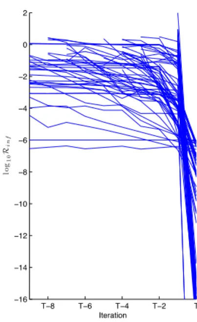
3.2 log10Rinf for the last 10 iterations of SQuIDapplied to infeasible instances. 71 4.1 Efficiency curves. . . 120

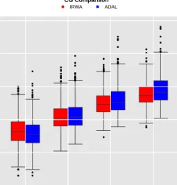
4.2 Box plot of CG steps for each duality gap threshold. . . 121

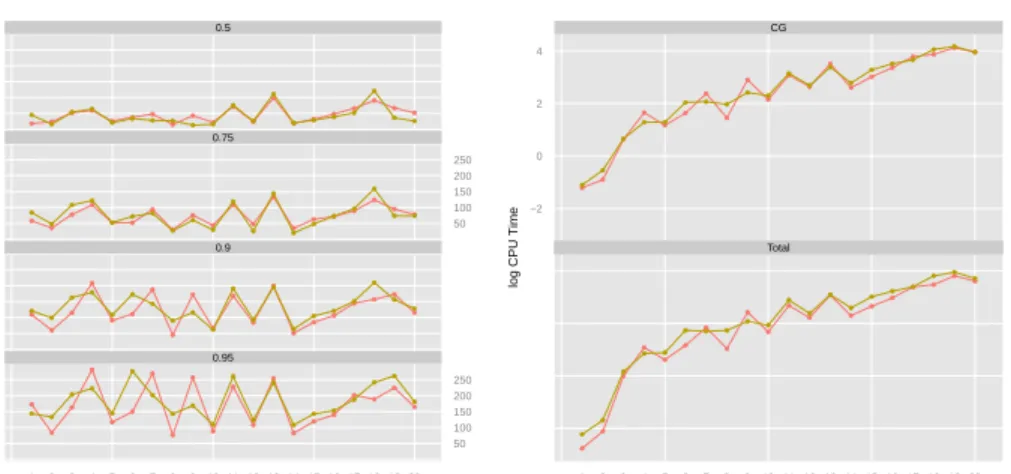
4.3 CG steps for each duality gap and CPU time plot as dimension increases. . 122

4.4 CG Steps and Objective function Comparison. . . 124

4.5 Sparsity of the Solutions . . . 125

4.6 Performance of normal IRWA and Accelerated IRWA . . . 125

5.1 Performance profile of ADAL-SQO and CPLEX-SQO . . . 154

(11)

Abstract

The primary focus of this dissertation is the design, analysis, and implementation of numer-ical methods to enhance Sequential Quadratic Optimization (SQO) methods for solving nonlinear constrained optimization problems. These enhancements address issues that challenge the practical limitations of SQO methods.

The first part of this dissertation presents a penalty SQO algorithm for nonlinear constrained optimization. The method attains all of the strong global and fast local convergence guarantees of classical SQO methods, but has the important additional feature that fast local convergence is guaranteed when the algorithm is employed to solve infeasible instances. A two-phase strategy, carefully constructed parameter updates, and a line search are employed to promote such convergence. The first-phase subproblem determines the reduction that can be obtained in a local model of constraint violation. The second-phase subproblem seeks to minimize a local model of a penalty function. The solutions of both subproblems are then combined to form the search direction, in such a way that it yields a reduction in the local model of constraint violation that is proportional to the reduction attained in the first phase. The subproblem formulations and parameter updates ensure that near an optimal solution, the algorithm reduces to a classical SQO method for constrained optimization, and near an infeasible stationary point, the algorithm reduces to a (perturbed) SQO method for minimizing constraint violation. Global and local convergence guarantees for the algorithm are proved under reasonable assumptions and numerical results are presented for a large set of test problems.

In the second part of this dissertation, two matrix-free methods are presented for ap-proximately solving exact penalty subproblems of large scale. The first approach is a novel

(12)

iterative re-weighting algorithm (IRWA), which iteratively minimizes quadratic models of relaxed subproblems while simultaneously updating a relaxation vector. The second ap-proach recasts the subproblem into a linearly constrained nonsmooth optimization problem and then applies alternating direction augmented Lagrangian (ADAL) technology to solve it. The main computational costs of each algorithm are the repeated minimizations of con-vex quadratic functions, which can be performed matrix-free. Both algorithms are proved to be globally convergent under loose assumptions, and each requires at most O(1/ε2) iterations to reach ε-optimality of the objective function. Numerical experiments exhibit the ability of both algorithms to efficiently find inexact solutions. Moreover, in certain cases, IRWA is shown to be more reliable than ADAL.

In the final part of this dissertation, we focus on the design of the penalty parameter updating strategy in penalty SQO methods for solving large-scale nonlinear optimization problems. As the most computationally demanding aspect of such an approach is the computation of the search direction during each iteration, we consider the use of matrix-free methods for solving the direction-finding subproblems within SQP methods. This allows for the acceptance of inexact subproblem solutions, which can significantly reduce overall computational costs. In addition, such a method can be plagued by poor behavior of the global convergence mechanism, for which we consider the use of an exact penalty function. To confront this issue, we propose a dynamic penalty parameter updating strategy to be employed within the subproblem solver in such a way that the resulting search direction predicts progress toward both feasibility and optimality. We present our penalty parameter updating strategy and prove that does not decrease the penalty parameter unnecessarily in the neighborhood of points satisfying certain common assumptions. We also discuss two matrix-free subproblem solvers in which our updating strategy can be readily incorporated.

(13)

Chapter 1 Introduction

Mathematical constrained optimization has grown in recent decades to become one of the most important and influential tools in applied mathematics. However, the classes of nonlinear optimization (NLO) problems that can be solved analytically are extremely limited, especially due to issues such as potentially incompatible constraints, large problem size, nonconexity and degeneracy. As a result, computational optimization methods that can tackle those issues are critical for solving the complex problems arising in practice. In this dissertation we present techniques for addressing issues related to incompatible constraints and large scale problems.

Infeasibility detection, the first focus of this dissertation, is the process of reporting a

valid certificate of infeasibility when given an infeasible optimization problem. Typically, such a certificate is given by a stationary point of constraint violation, thus named an

infeasible stationary point. To rapidly detect infeasibility of the constraints is an important

issue as many contemporary methods either fail or require an excessive number of iterations and/or function evaluations before being able to detect that a given problem instance is infeasible. As a result, modelers are forced to wait an unacceptable amount of time, only to be told eventually (if at all) that model and/or data inconsistencies are present. Rapid infeasibility detection is also important in techniques including branch-and-bound methods for nonlinear mixed-integer and parametric optimization, as algorithms for solving

(14)

such problems often require the solution of a number of nonlinear subproblems. Slow infeasibility detection by such algorithms can create huge bottlenecks.

The second focus of this dissertation is the challenge of solving large-scale problems. In particular, we focus on solvers for NLO algorithm subproblems. Along with other various NLO methods, Sequential Quadratic Optimization (SQO), commonly known as SQP, has been a standard technique for solving constrained NLO problems for decades. With an appropriate globalization mechanism, SQO methods can converge from remote starting points. They are also revered for their fast local convergence guarantees and impressive practical performance. SQO methods also enjoy the characteristics of being able to be warm-started effectively and providing highly accurate solutions. However, the applicability of SQO has traditionally be limited to small-to-medium-scale problems. This is mainly because a sequence of inequality-constrained Quadratic Optimization (QO) subproblems of the same size as the origin problem need to be solved. This issue has been a persistent challenge in SQO when applied to large-scale problems. However, in many situations, an accurate solution to the subproblem of a SQO method is not necessarily needed. In fact, an approximate solution with a relatively accurate estimate of the active-set or yielding sufficient improvement toward optimality or feasibility is often adequate to ensure progress of the algorithm. This fact motivates us to craft methods that can rapidly find inexact solutions of SQO subproblems.

The acceptance of inexact subproblem solutions offers the possibility of terminating the subproblem solver early, perhaps well before an accurate solution has been computed. This characterizes the types of strategies that we focus on in the third part of this thesis. Recently, some work has been done to provide global convergence guarantees for SQP methods that allow inexact subproblem solves [27]. However, the practical efficiency of such an approach remains an open question. A critical aspect of any implementation of such an approach is the choice of subproblem solver. This is the case as the solver must be able to provide good inexact solutions quickly, as well as have the ability to compute highly accurate solutions—say, by exploiting well-chosen starting points—in the

(15)

neighborhood of a solution of the NLO. In addition, while a global convergence mechanism such as a merit function or filter is necessary to guarantee convergence from remote starting points, an NLO algorithm can suffer when such a mechanism does not immediately guide the algorithm toward promising regions of the search space. To confront this issue when an exact penalty function is used as a merit function, we propose a dynamic penalty parameter updating strategy to be incorporatedwithin the subproblem solver so that each computed search direction predicts progress toward both feasibility and optimality. This strategy represents a stark contrast to previously proposed techniques that only update the penalty parameter after a sequence of iterations [40] or at the expense of numerous subproblem solves within a single iteration [19, 13].

Overall, in this dissertation, we present algorithms for addressing issues related to infeasibility, the challenge of solving large scale problems, and complicating factors involved in updating penalty parameters. Specifically, this dissertation includes the following:

1. First, we develop, analyze, and discuss the implementation of a globally convergent SQO framework. Emphasis is placed on a solid theoretical foundation for its ability to rapidly converge to an infeasible stationary point in infeasible cases and an opti-mal solution in feasible cases. To our knowledge, this is a novel feature that most contemporary methods do not possess.

2. Second, we design, analyze, and compare two matrix-free algorithms for inexactly solving penalty QO subproblems in a generic penalty SQO framework. Both algo-rithms are able to rapidly find good inexact solutions. Our primary contribution is a new iterative-reweighting algorithm, for which we present a convergence proof and complexity analysis.

3. Finally, we introduce a basic penalty SQO algorithm that will form the framework for which we will introduce our penalty parameter updating strategy and matrix-free subproblem solvers. We discuss implementations of our methods and the results of extensive numerical experiments. Our main contribution is a novel technique for

(16)

ren-dering an appropriate value of the penalty parameter while solving the subproblem. The structure of this dissertation is as follows. Chapter 2 discusses some background of nonlinear optimization methods, including the contemporary solvers and techniques related to the topics in this dissertation. In Chapter 3 we develop and analyze our proposed penalty-SQO method and investigate its global and local convergence behavior for both feasible and infeasible cases under common conditions. Chapter 4 presents two matrix-free solvers that can quickly find an inexact solution for subproblems with an exact penalty term. In Chapter 5, we propose an updating strategy for the penalty parameter while solving the SQO subproblem. Final remarks and comments on all of the methods in this dissertation are presented in Chapter 6.

(17)

Chapter 2 Background

2.1 Sequential Quadratic Optimization

We frame this dissertation in the context of the generic constrained NLO

min x f(x) s.t.      cE(x) = 0 cI(x)≤0 (2.1.1)

wheref :Rn→R,cE :Rn→RmE, andcI :Rn→RmI are continuously differentiable. In this dissertation, we are particularly interested in problems where the constraints may be infeasible, or the number of variables nand the number of constraintsm:=mE+mI are

very large.

Among algorithms for solving NLO (2.1.1), SQO method has become one of most powerful methods. Ever since 1963, when it was first proposed by Wilson [82], SQO has evolved into a powerful class of methods for a wide range of constrained optimization problems. Define the Lagrangian to (2.1.1) as

(18)

where λ = (λE, λI) are the Lagrange multipliers. In a basic SQO approach, the search

direction is defined as the solution to the following Quadratic Optimization (QO) subprob-lem, of which the objective function is a quadratic approximation to the Lagrangian at an iterate xk, and the constraints are the linearizations of these in (2.1.1) at xk:

min d ∇f(x k₎T_d₊1 2d T_Hk_d s.t.      cE(xk) +∇cE(xk)Td= 0, cI(xk) +∇cI(xk)Td≤0. (2.1.2)

Here Hk is the exact or approximate Hessian of L(x, λ) at (xk, λk) with respect tox. SQO variants typically enjoy global convergence guarantees under certain common sets of assumptions when globalization techniques are employed. Early global convergence proofs were accomplished in [47, 68], which still provide the foundations for proving global convergence for many SQO methods. When explicit second-order derivative information is used, one can show that SQO methods behave like Newton’s method to solve the Karush-Kuhn-Tucker (KKT) conditions for the NLO problem (2.1.1) including only the active constraints at the solution. This result is given by [71], which serves as the foundation for proving the local convergence rate for many SQO methods. SQO is famous for its fast local convergence in the neighborhood of a solution point satisfying common assumptions and an appropriate constraint qualification.

2.2 Contemporary Nonlinear Optimization Solvers

With the growing importance of optimization in many areas, researchers have implemented many successful optimization algorithms into off-the-shelf solvers, enabling people from different fields to conveniently apply the solvers for their own applications. Among many existing most successful NLO solvers, we focus on the software packagesIpopt[78],Knitro

[16, 18, 80], and Filter [36]. All of them implement either an SQO or an Interior Point

(19)

NLO problems. Next we review the methods implemented in these three solvers. Detailed descriptions of other solvers such as Lancelot [25], Snopt [40] and Loqo [50] are not included.

The basic structure of Ipopt is a primal-dual IP method framework, which solves a

sequence of barrier problems with monotonically decreasing barrier parameters. For each value of the barrier parameter, the KKT system of the barrier problem is attacked by a damped Newton method to obtain the search direction. Then a step size is determined by evaluating the progress toward optimality along the search direction using a filter technique.

Knitrohas three solvers for users to choose: Knitro-Direct,Knitro-CG, and Knitro

-Active, with default option Knitro-Direct. Knitro-Direct implements the IP method proposed in [80], which solves a sequence of barrier problems to obtain an optimal solution. Upon computing the search direction for a given barrier problem, a backtracking line search is employed to determine the step size. The algorithm implemented inKnitro-CGis also an

IP method, though it differs in that the search directions are obtained by (approximately) solving a QO subproblem with a trust region constraint. The final Knitro algorithm,

Knitro-Active, is a sequential linear-quadratic programming algorithm. It first solves a Linear Optimization (LO) subproblem, which ends up with a set of “working” constraints (constraints are that satisfied as equalities) at the LO solution. This working set is used to formulate an equality-constrained QO subproblem. The search direction is a combination of the solutions of the LO subproblem and the QO subproblem.

Filter employs a SQO method, computing the search direction by solving a QO

subproblem within a trust-region. A filter technique is used to decide whether the trial step should be accepted or rejected.

2.3 Infeasibility Detection in Contemporary Solvers

In theory, SQO methods can often guarantee global convergence from remote starting points to infeasible stationary points in addition to global and fast local convergence for

(20)

feasible problems. For example, see the trust-region SQO method in [8] or the penalty line search SQO methods in [19, 21]. For those methods, it is shown that in the neighborhood of a solution point satisfying common assumptions, fast local convergence to feasible optimal solutions can be attained. However, most contemporary SQO methods make no attempt to achieve a theoretical fast rate of convergence to stationary points in the infeasible case. Rapid infeasibility detection can be shown by [13], though a major deficiency in that algorithm is that perhaps many QO subproblems are required to be solved in each iteration to drive fast local convergence.

For an algorithm to be robust and efficient in all practical situations, it should be able to return a certificate of infeasibility when given an infeasible instance of the NLO problem (2.1.1). Such a certificate can be developed, for example, through a measure of infeasibility of the constraints. For our purposes, we consider the following`1-norm constraint violation

measure: v(x) :=X i∈E |ci(x)|+ X i∈I max_{ci(x),0}. (2.3.1)

Other types of constraint violation measures can be obtained by choosing different norms; e.g., `2-norm-squared violation v2(x) := P_i∈E(ci(x))2 +P_i∈I(max{ci(x),0})2 and the

`∞-norm violation v∞(x) = max{|ci(x)|, i ∈ E; max{ci(x),0}, i ∈ I}. Different measures

may lead to distinct behavior when incorporated into an algorithm, but a discussion of these issues is outside the scope of this dissertation. If there is no point satisfying the constraints of problem (2.1.1), then algorithms should be designed to return a point min-imizing constraint violation, i.e., in such cases, they should find the optimal solution to the following infeasibility problem:

min

x v(x). (2.3.2)

In practice, the priority for such an algorithm is to locate a stationary point for the NLO problem (2.1.1), but if that is deemed unattainable, then the algorithm should at least guarantee that a stationary point for the infeasibility problem (2.3.2) (i.e., a stationary point for v) will be found. A point that is locally stationary for the infeasibility problem

(21)

(2.3.2) but infeasible for NLO (2.1.1) is called an infeasible stationary point for (2.1.1), and the detection of such a point is a valid certificate of infeasible for problem (2.1.1). We are aware that finding an infeasible stationary point does not mean that the constraints of (2.1.1) are incompatible, but merely means they are locally inconsistent.

While many contemporary solvers have its infeasibility detection mechanism, in prac-tice they may often fail to locate infeasible stationary points, or at least fail to do so in a timely manner. In some situations, this inefficiency may be due to the use of a “switching” technique to tackle potentially infeasible problems. The main intent of such algorithms is to attempt to solve the NLO problem (2.1.1) until it has been determined that further progress cannot be obtained, at which point they revert to solving the infeasibility prob-lem (2.3.2) directly. That is, they revert to attempting to improve constraint satisfaction during afeasibility restoration phase. If sufficient progress in minimizing constraint viola-tion is attained in the restoraviola-tion phase, then the method returns to the main algorithm; otherwise, an infeasible stationary point may be detected. Such switching approaches are often effective, but they may lead to inefficiencies for infeasible cases or even certain types of feasible problems. The main reason for this is that, during the feasibility restoration phase, an algorithm may obtain a reduction in constraint violation, but at the same time it may be moving away from the set of optimal solutions. (Specifically, by ignoring the objective function completely during the feasibility restoration phase, the method may impair its overall progress.) If such an occurrence happens many times, the cost may be numerous iterations before escaping this cycle and moving to a new area or claiming infeasibility. Another inherent difficulty with a switching approach is that it is not easy to determine when to make a switch between the two phases. All of this motivates us in Chapter 3 to craft methods that can balance the two tasks of attaining optimality and constraint violation minimization without the use of a switching technique.

Another method for infeasibility detection involves the use of a penalty function. If the associated penalty parameter tends to an extreme value, then the algorithm transitions to minimizing constraint violation. We believe that this is a reasonable approach, but

(22)

may also be inefficient if the convergence of the parameter to its extreme value occurs too slowly.

In the remainder of this subsection, we illustrate performance of the infeasibility de-tection techniques implemented in Ipopt, Knitroand Filter. InIpopt, the restoration

phase is triggered whenever the KKT system is ill-conditioned or the line search procedure ends up with a tiny step size. In the restoration phase, it improves constraint satisfaction by solving an `2-norm feasibility problem with an additional proximal term in the

objec-tive which prevents the new iterate from straying far from the previous iterate. This is motivated by the concern that the restoration phase may impair overall progress if left unchecked. Infeasibility is detected when an insufficient improvement in the restoration phase is obtained. Otherwise, it reverts to the optimization phase with a point that is closer to feasibility.

As inIpopt,Knitro-Directhandles infeasibility detection via a condition on the step

size. If it is too small, then the algorithm reverts to Knitro-CG. Infeasibility detection in Knitro-CGis handled through updates of a penalty parameter, which may tend to infinity in order to place an increasingly higher priority on minimizing constraint violation. In

Knitro-Active, infeasibility is detected whenever the penalty parameter tends to infinity and the minimizer of an `1-norm model of the linearized constraints does not lead to an

improvement in feasibility.

InFilter, when an infeasible QO is encountered, the algorithm turns to a feasibility restoration phase. Before entering the restoration phase, their QO solver, an active set method, returns a solution with some linear constraints being feasible and some infeasible. Consider the case where only inequalities exist in (2.1.1). In the restoration phase, the constraint index set _I is partitioned into two sets, call them _I1(xk) and I2(xk). The first

set _I1(xk) contains all the linear feasible constraints, and the other, I2(xk), contains the

remaining indices, i.e., the linear infeasible constraints. While keeping the feasible linear constraints feasible, they minimize the `1 violation of the linear infeasible constraints.

(23)

method applied to such a problem. The restoration phase is exited whenever an iterate is determine at which the linearized constraints are all feasible. Otherwise, the algorithm, if it eventually detects infeasibility, returns a stationary point to the minimization of the violation of constraints in _I1(xk), while satisfying the remaining constraints. Therefore,

this type of infeasible stationary point is defined as one being stationary for the partial constraint violation measure

X

i∈I1(xk₎

max_{ci(x),0_} (2.3.3)

subject to the constraints ci₍_x₎_≤₀_{, i}_{∈ I}

2(xk).

Overall, the solvers described above use heuristics to handle infeasibility, mostly ap-plying a switching technique of the type previously mentioned. To show the performance of their strategies in practice, we provide a few small-scale examples (each with only two or three variables), all of which are infeasible and have the infeasible stationary point lo-cated at the origin. Typically, algorithms for NLO require a few assumptions to guarantee nice convergence properties: regularity, which means the gradients of the equality con-straints and active inequality concon-straints are linearly independent;strict complementarity, which requires the Lagrange multipliers for the equality constraints and active inequal-ity constraints to be nonzero; second-order sufficiency, which implies the Hessian of the Lagrangian function is (sufficiently) positive definite on the null space of gradients of the equality constraints and active inequality constraints. In order to have a variety of inter-esting test problems, the ones we have constructed satisfy different combinations of these assumptions (when observed in the context of the infeasibility problem (2.3.2) after slack variables are added to produce a constrained problem); in total we end up with eight different combinations which are listed in the Table 1 (Y=Yes, N=No). For Example 4 and Example 6 where the regularity condition does not hold, we observe that the multi-pliers cannot be uniquely determined, and some of them violate strictly complementarity. Therefore, it is not possible to create an instance with the regularity condition violated and strictly complementarity always satisfied, so we indicate Y/N for strict complementarity

(24)

for such cases. The formulations of these examples are given in Appendix 1. Another problem, Example 9 — which is not mentioned in the table — is a feasible problem for which we find some curious results from Filter.

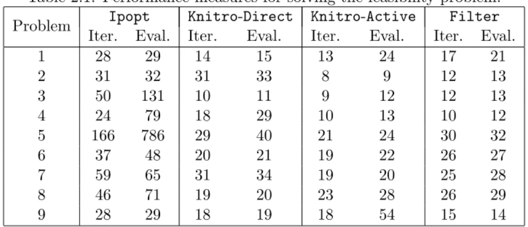
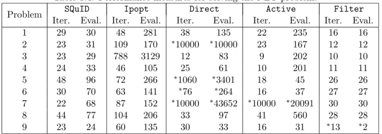
If the infeasibility of these examples is known a priori, then the user can directly apply the solvers to minimize the constraint violation. Table 2.1 provides these test results, where Iter. denotes the number of iterations and Eval. denotes the function evaluation counts. These solvers mostly require 20-30 iterations and function evaluations. Now suppose the infeasibility of these examples is not known by the user, so the solvers are tasked to solve the given NLO problems as they are stated in the Appendix. The performance information for this case without any presolve phase is provided in Table 2.2, where an asterisk means either the maximum iterations are exceeded or wrong information (e.g., that the problem is feasible) is reported to the user. The results overall seem unimpressive and far from the results in Table 2.2. We did not include the results of Knitro-CG, Lancelot, Snopt,

and Loqo on these examples in the table since they always ran out of iterations without

detecting infeasibility. The one solver that does produce acceptable-looking results is

Filter, it reports correct information rapidly but fails to provide an accurate infeasible stationary point. For Example 9, Filter reports the problem is locally infeasible at the point (−2.4109,−0.1012), but this is not actually an infeasible stationary point.

For cases where function evaluations are expensive or the problem scale is large, these solvers may run for hours or days without producing useful results, or, in the case of

Filter, it may correct infeasible quickly, but incorrectly on certain problems. Therefore,

one can see that nearly all these solvers may struggle for detecting infeasibility in practice.

2.4 QO Subproblems in Contemporary Solvers

There may be numerous issues arising when using subproblem (2.1.2). First, the con-straints may be inconsistent, which makes such a basic SQO subproblem not well-defined in practice. In the past decades, various ingredients have been proposed to enhance SQO methods to avoid this difficulty. Generally, many of them focus on two aspects: how to

(25)

Table 2.1: Performance measures for solving the feasibility problem.

Problem Ipopt Knitro-Direct Knitro-Active Filter

Iter. Eval. Iter. Eval. Iter. Eval. Iter. Eval.

1 28 29 14 15 13 24 17 21 2 31 32 31 33 8 9 12 13 3 50 131 10 11 9 12 12 13 4 24 79 18 29 10 13 10 12 5 166 786 29 40 21 24 30 32 6 37 48 20 21 19 22 26 27 7 59 65 31 34 19 20 25 28 8 46 71 19 20 23 28 26 29 9 28 29 18 19 18 54 15 14

Table 2.2: Performance measures for solving the NLO problem.

Problem Ipopt Knitro-Direct Knitro-Active Filter

Iter. Eval. Iter. Eval. Iter. Eval. Iter. Eval.

1 48 281 38 135 22 235 16 16 2 109 170 ∗10000 ∗10000 23 167 12 12 3 788 3129 12 83 9 202 10 10 4 46 105 25 61 10 201 11 11 5 72 266 ∗1060 ∗3401 18 45 26 26 6 63 141 ∗₇₆ ∗₂₆₄ ₁₆ ₃₇ ₂₇ ₂₇ 7 87 152 ∗10000 ∗43652 ∗10000 ∗20091 30 30 8 104 206 33 97 41 560 28 28 9 60 135 30 33 16 31 ∗₁₃ ∗₂

determine a step, and how to evaluate the improvement made by a step. For the former aspect, modern SQO methods involve varying techniques, typically depending on whether the method is based on a line search or trust-region approach. Both of them need some “mechanism” to evaluate the progress made by a step, of which there are commonly two kinds: a filter techinique or a penalty function formed by

φ(x;ρ) =ρf(x) +v(x).

By blending different options for all of these aspects, researchers have developed different versions of SQO, such as penalty SQO methods with line search (see [19] for example), penalty trust region SQO methods (see [35] for example), filter SQO methods with line search (see [79] for example), and filter trust region SQO methods (see [37] for example).

(26)

Each of these techniques yields different practical behavior.

Various other techniques are also proposed to handle other specific issues in SQO methods. The method of S`1QP [35], also known as the elastic SQO method [4, 40] was

proposed to overcome the difficulties caused by the inconsistency of the subproblem (2.1.2) constraints. The subproblem in such a penalty SQO method is given by

min d,r,s,tρ∇f(x k₎T_d₊1 2d T_Hk_d₊_eT₍_r₊_s_{) +}_eT_t s.t.                      cE(xk) +∇cE(xk)Td=r−s, i∈ E cI(xk) +∇cI(xk)Td≤t, i∈ I r_≥0, s_≥0, t_≥0 kdk∞≤∆k (2.4.1)

where constant ρ > 0 is penalty parameter. This subproblem is always feasible, meaning that the search direction is always well-defined.

Clearly, the major computational cost in an SQO method is the solution of the QO subproblems, which generally involve equality and inequality constraints. On one hand, near the optimal solution, once the active set is determined, the QO subproblems then reverts to equality constrained QOs, which can be solved by solving a system of linear equations. As a result, fast local convergence can be achieved when active set method is employed as the subproblem solver. This feature has led to active set SQO methods being considered powerful solvers for small-to-medium-scale NLOs.

On the other hand, the need of having to solve QO subproblems has prevented SQO methods from becoming an ideal option for large-scale problems. The existence of inequal-ities generally makes the QO subproblems difficult to solve. When active set QO solvers are used, the iterations needed for subproblems could be exponential with the number of constraints in the worst case. Consequently, the computational time grows rapidly when the problem size gets larger, and the method could even fail for large-scale cases in a timely manner.

(27)

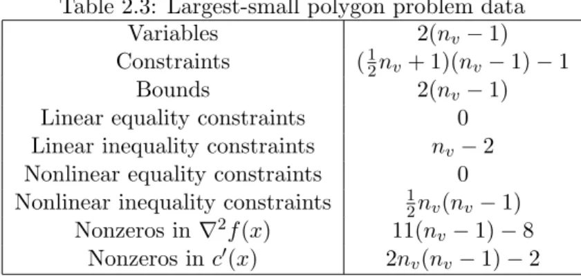
An illustration of such an effect can be found in the COPS test set report [29]. We use an example from [29] to show how the performance of an SQO solver could suffer from large problem sizes. The comparison is carried out on Filter,Knitro,Loqo,Minos, and Snopt. This example is to find the polygon of maximal area, among polygons with nv sides and diameter d ≤ 1. The problem size is summarized in Table 2.3. The test

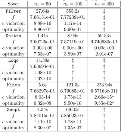
results are shown in Table 2.4, where the first row for each solver is the computational time,f, “cviolation” and “optimality” in the table represent the function value, constraint violation, and the optimality error at the final iterate, respectively. A _† mark means an incorrect result was obtained, and ‡ represents a failure within time limit. One can see from Table 2.4 that the computational time grows dramatically for Filter,Loqo,Minos, and Snoptwhen the problem size becomes larger. They fail to solve the problem within the time limit, or even return an incorrect result (Minos withnv = 200). Another aspect

to notice is that the dramatic growth in the computational time of Filter, which may be

due to the fact that an active set QO method is employed in this solver [36]. Among all the NLO solvers, Knitrois reported to be most stable, with slow growth in computation time. This is mainly due to the fact that all the three methods implemented in Knitro

solve subproblems of linear equations, linear optimization, and equality constrained QO which is equivalent to linear equations. The same effect can be observed in most of the other examples in [29]. Therefore, the performance of SQO solvers on large-scale problems relies critically on the efficiency of the QO solvers.

Table 2.3: Largest-small polygon problem data

Variables 2(nv−1)

Constraints (1₂nv+ 1)(nv−1)−1

Bounds 2(nv−1)

Linear equality constraints 0

Linear inequality constraints nv−2

Nonlinear equality constraints 0

Nonlinear inequality constraints 1

2nv(nv−1)

Nonzeros in∇2_f₍_x₎ ₁₁₍_n

v−1)−8

Nonzeros in c0(x) 2nv(nv−1)−2

(28)

Table 2.4: Performance on largest small polygon problem

Sover nv = 50 nv = 100 nv = 200

Filter 27.64s 555.2s _‡

f 7.66131e-01 7.77239e-01 _‡

c violation 8.88e-16 1.17e-14 ‡

optimality 8.96e-07 9.90e-07 _‡

Knitro 1.41s 8.99s 59.53s

f 7.60725e-01 7.37119e-01 6.740980e-01

c violation 0.00e+00 0.00e+00 0.00e+00

optimality 7.53e-07 3.99e-07 2.01e-07

Loqo 14.39s ‡ ‡

f 7.63694e-01 _‡ _‡

c violation 1.08e-10 _‡ _‡

optimality 1.02e-10 ‡ ‡

Minos 5.6s 121.3s 223.94s

f 7.66297e-01 6.79085e-01 6.57163e-01_†

c violation 8.03-14 1.75e-13 2.66e-15_†

optimality 6.32e-08 9.50e-10 9.55e-02†

Snopt 4.34s 69.35s ‡

f 7.84015e-01 7.85023e-01 _‡

c violation 1.11e-10 1.78e-11 _‡

optimality 8.30e-07 1.35e-07 ‡

not necessary. If a given inexact setp can make sufficient progress toward a solution of the NLO, then global convergence can still be guaranteed. A variety of SQO methods with inexactness in step computations have been proposed recently [52, 58, 48]. The conditions that guarantee the global convergence of inexact SQP steps are discussed in [20]. This feature of the QO subproblem provides the foundation of applying SQO methods to large-scale applications.

2.5 Penalty Parameter Update in Contemporary Methods

The `1 penalty function φ(x;ρ) has been proved to be an exact penalty function of the

NLO problem (2.1.1). This result is given by the following theorem [84, Theorem 17.3]

Theorem 2.5.1. Suppose that x∗ is a strict local solution of the nonlinear optimization

(29)

multipliers λ∗. Then x∗ is a local minimizer of φ(x;ρ) for all ρ < ρ∗, where _ρ1∗ =kλ∗k∞.

If, in addition, the second-order sufficient conditions hold and ρ < ρ∗ then x∗ is a strict

local minimizer of φ(x;ρ).

Exact penalty methods, such as S`1QP, solve a local approximation model of φ(x;ρ)

such as min kdk∞∈∆k ρ_∇f(xk)Td+1 2d T_Hk_d₊X i∈E |ci(xk)+∇ci(xk)Td|+ X i∈I max_{ci(xk)+∇ci(xk)Td,0},

which is equivalent to subproblem (2.4.1). Therefore, exact penalty methods are well as effective techniques for handling the inconsistent constraints arising in the QO subproblem. Based on Theorem 2.5.1, the penalty parameter ρ is updated at each iteration to prevent the convergence to an undesirable point. Despite advantages of exact penalty methods, their performance can be significantly affected by the penalty parameter, making it difficult to keep efficient over a wide range of problems. Therefore, the penalty parameter updating strategy is the critical point of constructing penalty methods. It has proved difficult to designing successful updating strategy.

Early updating strategies may solve the subproblem for a finite sequence of decreasing

ρ [40], or scale down the penalty parameter by the magnitude of the multipliers [34]. This strategy can result in inefficient behavior and also requires heuristics to terminate the update. Various approaches have been recently proposed to handle this situation. In [21], the penalty parameter ρ is updated at every iteration so that sufficient progress toward feasibility and optimality is guaranteed to first order. They solve an auxiliary LO subproblem to evaluate the progress. Steering rules[19] and other methods [13] also require the penalty parameter to guarantee sufficient improvement on feasibility and optimality. Multiple subproblems may be solved per iteration with decreasing penalty parameter until the desirable value is found.

(30)

Chapter 3 An SQO Algorithm with Rapid

Infeasibility Detection

3.1 Introduction

Sequential quadratic optimization (SQO) methods are known to be extremely efficient when applied to solve nonlinear constrained optimization problems [47, 67, 82]. Indeed, it has long been known [7, 8, 9] that with an appropriate globalization mechanism, SQO methods can guarantee global convergence from remote starting points tofeasible optimal solutions, or toinfeasible stationary points if the constraints are incompatible. One of the main additional strengths of SQO is that in the neighborhood of a solution point satisfying common assumptions and an appropriate constraint qualification, fast local convergence

tofeasible optimal solutions can be attained [70].

Despite these important and well-known properties of SQO methods, there is an im-portant feature that many contemporary SQO methods lack, and it is for this reason that the algorithm in this chapter has been designed, analyzed, and tested. Specifically, in addition to possessing the convergence guarantees mentioned in the previous paragraph, we have proved that the algorithm proposed in this chapter yields fast local convergence

(31)

There are two main novel features of our algorithm. Most importantly, it is an algo-rithm that possesses global and local superlinear convergence guarantees for feasible and

infeasible problemswithout having to resort to feasibility restoration. This feature, in that a single approach is employed for solving both feasible and infeasible problems, means that the algorithm avoids many of the inefficiencies that may arise when contemporary methods are employed to solve problems with incompatible constraints. The second novel feature of our algorithm is that it is able to attain these strong convergence properties with at most two quadratic optimization (QO) subproblem solves per iteration. This is in contrast to recently proposed methods that provide rapid infeasibility detection, but only at a much higher per-iteration cost.

In the following section, we compare and contrast our approach with recently proposed SQO methods, focusing on properties of those methods related to infeasibility detection. We then present our algorithm in_§3.2 and analyze its global and local convergence prop-erties in _§3.3. Our numerical experiments in_§5.6 illustrate that an implementation of our algorithm yields solid results when applied to a large set of test problems.

We remark at the outset that we analyze the local convergence properties of our algo-rithm under assumptions that are classically common for analyzing that of SQO methods. We explain that our algorithm can be backed by similarly strong convergence guaran-tees under more general settings (see our discussion in §3.3.3), but have made the con-science decision to use these common assumptions to avoid unnecessary distractions in the analysis. Overall, the main purpose of this chapter is to focus on the novelties of our algorithm—which include the unique formulations of our subproblems, our use of separate multiplier estimates for the optimization and a corresponding feasibility problem, and our unique combination of updates for the penalty parameter—which provide our algorithm with global and fast local convergence guarantees on both feasible and infeasible problem instances.

(32)

3.1.1 Literature Review

Our algorithm is designed to act as an SQO method for solving an optimization problem when the problem is feasible, and otherwise it is designed to act as a perturbed SQO method [26] for a problem to minimize constraint violation. In this respect, our method has features in common with those in the class of penalty-SQO methods [35] where search directions are computed by minimizing a quadratic model of the objective combined with a penalty on the violation of the linearized constraints. In such algorithms, if the penalty parameter is driven to an extreme value, then the algorithm transitions to solely minimizing constraint violation. We believe that this approach is reasonable, though there are two main disadvantages of the manner in which penalty-SQO methods are often implemented. One disadvantage is that the penalty parameter takes on all of the responsibility for driving constraint violation minimization. This leads to a common criticism of penalty methods, which is that the performance of the algorithm is too highly dependent on the penalty parameter updating scheme. The second disadvantage is that, if the penalty parameter is not driven to its extreme value sufficiently quickly, then convergence, especially for infeasible problems, can be slow. These disadvantages motivate us to design a method that reduces to a classical SQO approach for feasible problems, and where updates for the penalty parameter lead to rapid convergence in infeasible cases.

The immediate predecessor of our work is the penalty-SQO method proposed in [13]. In particular, the approach in [13] is also proved to yield fast local convergence guarantees for infeasible problems. That method does, however, have certain practical disadvantages. The most significant of these is that, particularly in infeasible cases, the method may require the solution of numerous QO subproblems per iteration. Indeed, near an infeasible stationary point, at least three QO subproblems must be solved. The first will reveal that for the current penalty parameter value it is not possible to compute a linearly feasible step, the second then gauges the progress toward linearized feasibility that can be made locally, and the third may produce the actual search direction. (In fact, if the conditions necessary for global convergence are not satisfied after the third QO subproblem solve, then even

(33)

more QO subproblem solves are needed until the conditions are satisfied.) In contrast, the algorithm proposed in this chapter solves at most two QO subproblems per iteration. It also relies less on the penalty parameter for driving constraint violation minimization, and involves separate multiplier estimates for the optimization and feasibility problems. This last feature of our algorithm—that of having two separate multiplier estimates—is quite unique for an optimization algorithm. However, we believe that it is natural as the optimization algorithm must implicitly decide which of two problems to solve: the given optimization problem or a problem to minimize constraint violation.

Our algorithm is a multi-phase active-set method that has similarities with other such methods that have been proposed over the last few decades. For instance, the method in [13] borrows the idea, proposed in [19] and later incorporated into the line-search method in [17], of “steering” the algorithm with the penalty parameter. Consequently, that method at least suffers from the same disadvantages as the method in [13] when it comes to infeasibility detection. More commonly, multi-phase SQO methods have taken the approach of solving a first-phase inequality-constrained subproblem—typically a lin-ear optimization (LO) subproblem—to estimate an optimal active set, and then solving a second-phase equality-constrained subproblem to promote fast convergence; e.g., see [21, 15, 23, 31, 32, 39]. A method of this type that solves two QO subproblems is that in [57], though again the second-phase subproblem in that method is equality-constrained as it only involves linearizations of constraints predicted to be active at an optimal solu-tion. Our algorithm differs from these in that we do no active-set prediction, and rather solve up to two inequality-constrained subproblems. The methods in [44, 45] involve the solution of up to three subproblems per iteration: one to compute a “predictor” step, one to compute a “Cauchy” step, and one to compute an “accelerator” step. In fact, various subproblems are proposed for the “accelerator” step, including both equality-constrained and inequality-constrained alternatives. Our algorithm differs from these in that ours is a line search method, whereas they are trust region methods, and our first-phase subprob-lem computes a pure feasibility step rather than one influenced by a local model of the

(34)

objective. This latter feature makes our method similar to those in [7, 8], though again our work is unique in that we ensure rapid infeasibility detection, which is not provided by any of the aforementioned methods besides that in [13]. Finally, we mention that multi-phase strategies have also been employed in interior-point techniques; e.g., see [14, 59].

3.2 Algorithm Description

We present our algorithm in the context of the generic nonlinear constrained optimization problem

minimize

x (minx ) f(x)

subject to (s.t.) cE(x) = 0, cI(x)≤0,

(3.2.1)

where f :Rn → R, cE :Rn → RmE, and cI :Rn →RmI are twice-continuously differen-tiable. If the constraints of (3.2.1) are infeasible, then the algorithm is designed to return an infeasibility certificate in the form of a minimizer of the`1 infeasibility measure of the

constraints; i.e., in such cases it is designed to solve

min

x v(x), where v(x) :=kcE(x)k1+k[cI(x)]

+_k

1. (3.2.2)

Here, for a vector c, we define [c]+ _{:= max}_{_c,₀_} _{and, for future reference, define [}_c_]− _:=

max{−c,0}(both component-wise). The priority is to locate a stationary point for (3.2.1), but in all cases the algorithm is at least guaranteed to find a stationary point for (3.2.2), i.e., a stationary point forv. We say a pointxis stationary forvif 0_∈∂v(x), where∂v(x) is the Clarke subdifferential of v atx [6, 24] (see [7] for a complete review of first-order theory for potentially infeasible problems).

Each iteration of our algorithm consists of solving at most two QO subproblems, up-dating a penalty parameter, and performing a line search on an exact penalty function. In this regard, the method is broadly similar to that proposed in [7]; however, the algorithm contains numerous refinements included to ensure rapid local convergence in both feasible and infeasible cases. In this section, we present the details of each step of the algorithm.

(35)

Of particular importance is the integration of our penalty parameter updates around the QO solves as this parameter is critical for driving fast local convergence for infeasible instances. A complete description of our algorithm is presented at the end of this section. We begin by describing the conditions under which our algorithm terminates finitely. In short, the algorithm continues iterating unless a stationary point for problem (3.2.1) has been found. We define such stationary points according to first-order optimality conditions for problems (3.2.1) and (3.2.2), all of which can be presented by utilizing the Fritz John (FJ) function for (3.2.1), namely

F(x, ρ, λ) :=ρf(x) +λETcE(x) +λITcI(x).

Here,ρ_∈R is an objective multiplier andλ, withλE ∈RmE andλI ∈RmI, are constraint multipliers. For future reference, we note thatρalso plays the role of the penalty parameter in the `1 exact penalty function

φ(x, ρ) :=ρf(x) +v(x). (3.2.3)

Our algorithm updates ρ and seeks stationary points for (3.2.1) through decreases inφ. One possibility for finite termination is that the algorithm locates a first-order optimal point for (3.2.1). First-order optimality conditions for problem (3.2.1) are

∇xF(x, ρ, λ) =ρ∇f(x) +∇cE(x)λE+∇cI(x)λI = 0,

cE(x) = 0, cI(x)≤0,

λI ≥0, λI·cI(x) = 0.

(3.2.4)

Here, _∇f : Rn → Rn is the gradient of f, [∇cE]T : Rn → RmE×n is the Jacobian of cE

(and similarly for [_∇cI]T), and for vectors a and b we denote their component-wise (i.e.,

Hadamard or Schur) product bya_·b, a vector with entries (a_·b)i =aibi. If (x∗, ρ∗, λ∗) with

(36)

it is a FJ point [53]. Of particular interest are those FJ points with ρ∗ > 0 as these correspond to Karush-Kuhn-Tucker (KKT) points for (3.2.1) [55, 56].

The other possibility for finite termination is that the algorithm locates a stationary point for (3.2.2) that is infeasible for problem (3.2.1). Hereinafter, defining eas a vector of ones (whose size is determined by the context), first-order optimality conditions for problem (3.2.2) are ∇xF(x,0, λ) =∇cE(x)λE+∇cI(x)λI = 0, −e≤λE ≤e, 0≤λI ≤e, (e+λE)·[cE(x)]−= 0, (e−λE)·[cE(x)]+= 0, λI·[cI(x)]−= 0, (e−λI)·[cI(x)]+= 0. (3.2.5)

If (x∗, λ∗) satisfies (3.2.5) and v(x∗) > 0, then we call (x∗, λ∗) stationary for (3.2.1); in particular, it is an infeasible stationary point. Despite the fact that such a point is infeasible for (3.2.1), it is deemed stationary as first-order information indicates that no further improvement in minimizing constraint violation locally is possible.

We now describe our technique for computing a search direction and multiplier esti-mates, which involves the solution of the QO subproblems (3.2.7) and (3.2.9) below. Once the details of these subproblems have been specified, we will describe an updating strategy for the penalty parameter that is integrated around these QO solves.

At the beginning of iteration k, the algorithm assumes an iterate of the form

(xk, ρk, λk,bλk) with ρk>0, −e≤λ

k

E ≤e, 0≤λ

k

I ≤e, and λbk_I ≥0. (3.2.6)

As all stationary points for (3.2.1) are necessarily stationary for the constraint violation measure v, we initiate computation in iteration k by seeking to measure the possible improvement in minimizing the following linearized model ofv atxk_:

(37)

Specifically, defining H(x, ρ, λ) as an approximation for the Hessian of F at (x, ρ, λ), we solve the following QO subproblem whose solution we denote as (dk, rk, sk, tk):

min (d,r,s,t)e T₍_r₊_s_{) +}_eT_t₊1 2d T_H₍_xk_,₀_{, λ}k₎_d s.t.              cE(xk) +∇cE(xk)Td= r−s cI(xk) +∇cI(xk)Td≤ t (r, s, t)_≥ 0. (3.2.7)

As shown in Lemma 3.3.2 in_§3.3.1, this subproblem is always feasible and, ifH(xk,0, λk) is positive definite, then the solution component dk is unique. In addition, dk yields a nonnegative reduction in l(_·;xk), i.e.,

∆l(dk;xk) :=l(0;xk)−l(dk;xk)≥0, (3.2.8)

where equality holds if and only ifxk is stationary forv. Upon solving subproblem (3.2.7) and setting

λk+1 with −e_≤λk+1_E _≤e and 0≤λk+1_I _≤e

as the optimal multipliers for the linearized equality and inequality constraints in (3.2.7), we check for termination at an infeasible stationary point. Specifically, we consider the constraint violation measure v and the following residual for (3.2.5):

Rinf(xk, λ k+1 ) := max_{k∇xF(xk,0, λ k+1 )_k∞, k(e₋λk+1_E )_·[cE(xk)]+k∞,k(e+λk+1_E )·[cE(xk)]−k∞, k(e−λk+1_I )·[cI(xk)]+k∞,kλk+1_I ·[cI(xk)]−k∞}. If Rinf(xk, λ k+1

) = 0 and v(xk) > 0, then (xk, λk+1) is an infeasible stationary point. Otherwise, as shown in Lemma 3.3.2 in §3.3.1, it follows that either v(xk) = 0 or dk is a

(38)

direction of strict descent for v fromxk.

Having measured, in a particular sense, the possible improvement in minimizing con-straint violation by solving the QO subproblem (3.2.7), the algorithm solves a second QO subproblem that seeks optimality. Denoting _Ek _and _Ik _{as the sets of constraints that}

are linearly satisfied at the solution of (3.2.7) (i.e., that have rk_i = sk_i = 0 for i _{∈ E} or

tk_i = 0 for i_{∈ I}, respectively), we require that the computed direction maintains this set of linearly satisfied constraints. The other linearly violated constraints in _Ek

c ∪ Ick (where

Ek

c := E \ Ek and Ick := I \ Ik) remain relaxed with slack variables whose values are

penalized in the subproblem objective. The value of the penalty parameter employed at this stage is the value forρkimmediately prior to this second phase subproblem, which for future notational convenience we denote as ρb

k_{. Overall, we solve the following regularized}

QO subproblem whose solution we denote as (dbk,r_bk_Ek c,sb k Ek c,bt k Ik c): min (d,r_Ek c,sEck,tIck) b ρk∇f(xk)Td+eT(rEk c +sEck) +e T_t Ik c + 1 2d T_H₍_xk_, b ρk,bλk)d s.t.              cEk(xk) +∇c_Ek(xk)Td= 0, c_Ek c(x k_{) +} ∇cEk c(x k₎T_d₌_r Ek c −sEck, c_Ik(xk) +∇c_Ik(xk)Td≤0, c_Ik c(x k_{) +}_∇_c Ik c(x k₎T_d_≤_t Ik c, (rEk c, sEck, tIkc)≥0. (3.2.9)

Upon solving (3.2.9) and setting

b λk+1 with −e≤λbk+1 Ek c ≤e, 0≤ b λk+1_Ik c ≤e, and b λk+1_Ik ≥0

as the optimal multipliers for the linearized equality and inequality constraints in (3.2.9), it is again appropriate to check for finite termination of the algorithm, this time with respect to the optimality conditions for (3.2.1). Given (xk, ρk,bλk+1) we consider the violation

measure v and the following residual corresponding to (3.2.4):

(39)

We prove in Lemma 3.3.4 in §3.3.1 that if the algorithm reaches this stage, then ρk is strictly positive. Thus, if Ropt(xk, ρk,λbk+1) = 0 and v(xk) = 0, then (xk, ρk,λbk+1) is a

KKT point for (3.2.1).

If the algorithm has not terminated finitely due to this last check of optimality, then the search directiondk is chosen as a convex combination of the directions obtained from subproblems (3.2.7) and (3.2.9). Given a constantβ _∈(0,1), our criterion for the selection of the weights in this combination is

∆l(dk;xk)≥β∆l(dk;xk). (3.2.10)

For w_∈[0,1], the reduction in l(_·;xk) obtained by

d(w) :=wdk+ (1−w)dbk (3.2.11)

is a piecewise linear function of w. If ∆l(dk;xk) = 0, then by the formulation of (3.2.9), we have ∆l(dbk;xk) = 0 and so (3.2.10) is satisfied byw= 0. Otherwise, if ∆l(d

k

;xk)>0, then since ∆l(d(1);xk) = ∆l(dk;xk)> β∆l(dk;xk), there exists a thresholdw∈[0,1) such that (3.2.10) holds for all w ≥w. We define wk as the smallest value in [0,1) such that (3.2.10) holds and set the search direction as dk_←_d₍_wk_).

We have presented our techniques for computing the primal search directiondkas well as new multiplier estimates λk+1 and λbk+1. Within this discussion, we have accounted

for finite termination of the algorithm and highlighted certain consequences of our step computation procedure (e.g., (3.2.8) and (3.2.10)) that will be critical in our convergence analysis. All that remains in the specification of our algorithm is our updating strategy for the penalty parameter and the conditions of our line search, which we now present. Note that with respect to ρ, an update is considered twice in a given iteration. The first time an update is considered is between the two QO subproblem solves, as it is at this point in the algorithm where the solution of (3.2.7) may trigger aggressive action toward infeasibility detection. The second time an update is considered is after the solution of

(40)

(3.2.9). The update considered at that time is representative of typical contemporary updating strategies, used to ensure a well-defined line search and global convergence of the algorithm.

Prior to solving the second subproblem (3.2.9) (and before fixing ρ_bk), we potentially modifyρkandbλk(computed in iterationk−1) to reduce the weight of the objectivef and

promote fast infeasibility detection. (Note thatρk andbλk will both influence the objective

of (3.2.9).) If the current iterate is infeasible and the reduction in linearized feasibility obtained by dk is small compared to the level of nonlinear infeasibility, then there is evidence that the algorithm is converging to an infeasible stationary point. In such cases, we consider modifyingρkbefore solving subproblem (3.2.9) so that the rest of the iteration places a higher emphasis on reducing constraint violation. A corresponding modification to

b

λk_{is also necessary to guarantee fast infeasibility detection (see Theorem 3.3.11). Defining}

constants θ_∈(0,1),κρ>0, andκλ >0, if v(xk)>0 and ∆l(dk;xk)≤θv(xk), (3.2.12) then we set ρk by ρk_←min_{ρk, κρRinf(xk, λ k+1 )2} (3.2.13)

and modify bλk so that

kbλk−λ

k

k ≤κλRinf(xk, λ k+1

)2. (3.2.14)

Otherwise, we maintain the current ρk and bλk. For satisfying (3.2.14), a simple approach

is to setλbk←α_λbλk+ (1−α_λ)λ

k

whereαλ is the largest value in [0,1] such that (3.2.14)

is satisfied. (This is the approach taken in our implementation described in _§5.6.)

Upon solving (3.2.9) and assuming the algorithm does not immediately terminate, we turn to a second update for ρ and our line search. For these purposes, we employ the `1

exact penalty function φ(recall (3.2.3)). At xk, a linear model ofφ(·, ρ) is

(41)

and the corresponding reduction in this model yielded by the search direction dk is

∆m(dk;xk, ρ) :=m(0;xk, ρ)₋m(dk;xk, ρ) =₋ρ_∇f(xk)Tdk+ ∆l(dk;xk). (3.2.15)

Prior to the line search, the new penalty parameterρk+1is set so that its reciprocal is larger than the largest multiplier (derived from (3.2.9)) and that the reduction ∆m(dk;xk, ρk+1) is at least proportional to ∆l(dk_;_xk_{). That is, we set} _ρk+1 _{so that}

ρk+1_kbλk+1k_∞≤1 (3.2.16)

and, for a given constant _∈(0,1), we have

∆m(dk;xk, ρk+1)_≥∆l(dk;xk). (3.2.17)

Given constants δ_∈(0,1) and ω_∈(0,1), (3.2.16) and (3.2.17) can be achieved by setting

ρk←min ( δρk, (1−) kbλk+1k∞ ) if ρkkbλk+1k_∞>1 (3.2.18) followed by ρk_←        δρk if ∆m(dk;xk, ρk)_≥∆l(dk;xk) andwk_≥ω; min δρk, ζk if ∆m(dk;xk, ρk)< ∆l(dk;xk), (3.2.19) where ζk:= (1−)∆l(d k_;_xk₎ ∇f(xk₎T_dk₊1 2(dk)TH(xk,ρb k_, b λk₎_dk,

and then setting ρk+1 _← ρk. Once ρk+1 has been set in this manner, we perform a backtracking line search along dk to determineαk such that, forη_∈(0,1), we have

(42)

Our proposed algorithm, hereinafter nicknamed SQuID , is presented as Algorithm 1. We claim that the algorithmic framework of SQuID is globally convergent for choices of subproblems other than (3.2.7). For instance, a linear subproblem with a trust region would be appropriate for determining the best local improvement in linearized feasibility; e.g., see [7, 8]. Under certain common assumptions, this choice should also allow for rapid local convergence for feasible problem instances. We present SQuID as solving two QO subproblems per iteration, however, as this choice also allows for rapid local convergence

forinfeasible instances, the main focus of this chapter. In particular, in the neighborhood

of an infeasible stationary point satisfying the assumptions of§3.3.3, it can be seen that as

ρk→0 andbλk→λ

k

, subproblem (3.2.9) produces SQO-like steps for the minimization of constraint violation, thus causing rapid convergence toward stationary points for v. This being said, efficient implementations of SQuID may avoid two QO solves per iteration.

For example, at (nearly) feasible points, one may consider skipping subproblem (3.2.7) entirely, as we do in our implementation described in _§5.6. For the purposes of this chapter, however, we analyze the behavior of SQuID as it has been presented.

Algorithm 1 SequentialQuadratic Optimizer with RapidInfeasibilityDetection

1: Chooseβ ∈(0,1),θ∈(0,1),κρ>0,κλ>0,∈(0,1),ω∈(0,1),δ ∈(0,1),η∈(0,1),

and γ _∈(0,1). Set k_←0 and choose (xk, ρk, λk,bλk) satisfying (3.2.6).

2: Compute (dk, rk, sk, tk, λk+1) as the optimal primal-dual solution for (3.2.7).

3: If R_inf(xk, λk+1) = 0 and v(xk) > 0, then terminate; (xk, λk+1) is an infeasible sta-tionary point for problem (3.2.1).

4: If (3.2.12) holds, then set ρk _{by (3.2.13) and}

b

λk _{so that (3.2.14) holds. Set}

b ρk _←_ρk_. 5: Compute (dbk,_br_Ek_k c,bs k Ek c,bt k Ik c, b

λk+1) as the optimal primal-dual solution for (3.2.9).

6: IfRopt(xk, ρk,bλk+1) = 0 and v(xk) = 0, then terminate; (xk, ρk,bλk+1) is a KKT point

for problem (3.2.1).

7: Setdk by (3.2.11) wherewk is the smallest value in [0,1) such that (3.2.10) holds.

8: Updateρk by (3.2.18), then by (3.2.19), and finally setρk+1 ←ρk.

9: Letαk be the largest value in _{γ0, γ1, γ2, . . .} such that (3.2.20) holds.

(43)

3.3 Convergence Analysis

The convergence properties of SQuID are the subject of this section. We prove the well-posedness of the algorithm along with global and local convergence results for feasible and infeasible problem instances. A few of the earlier results in this section are well-known in (nonsmooth) composite function theory, so for the sake of brevity we only provide citations for proofs.

3.3.1 Well-Posedness

We prove thatSQuID is well-posed in that each iteration is well-defined and, if the overall algorithm does not terminate finitely, then an infinite sequence of iterates will be produced. This can be guaranteed under the following assumption. (Note that for simplicity here and in _§3.3.2, we assume that subproblems (3.2.7) and (3.2.9) are convex. See_§3.3.3 for a discussion of how this assumption can be relaxed without sacrificing local superlinear convergence guarantees.)

Assumption 3.3.1. The following hold true for the iterates generated by SQuID:

(a) The problem functionsf,cE, andcI are continuously differentiable in an open convex

set containing _{xk_} and _{xk+dk_}.

(b) For all k, H(xk_,₀_{, λ}k₎ _and_H₍_xk_,

b

ρk_,

b

λk₎ _{are positive definite.}

Our first lemma reveals that₋∆l(d;xk) and ₋∆m(d;xk, ρ) respectively play the roles of surrogates for the directional derivatives of v and φ(_·.ρ) from xk along the direction

d. For a proof, see [6, Lemma 2.3]. We use the lemma to show that as long as a search directiondkyields a strictly positive reduction inl(_·, xk) (m(_·;xk, ρ)), then it is a direction of strict decrease forv (φ(·, ρ)).

Lemma 3.3.1. The reductions in l(·;xk) andm(·;xk, ρ) produced by dsatisfy