Exponential two step approach for Time Domain based Software Process
Control
ABSTRACT
Software Reliability Growth Model is a mathematical model of how the software reliability improves as faults are detected and repaired. In this paper we propose a control mechanism based on the cumulative quantity between observations of time domain failure data using mean value function of Goel-Okumoto model, which is based on Non Homogenous Poisson Process. The model parameters are estimated by a two step approach. Software reliability process can be monitored efficiently by using Statistical Process Control. Control charts are widely used for process monitoring. It assists the software development team to identify failures and actions to be taken during software failure process and hence, assures better software reliability.
General Terms
Software Engineering, Statistical Reliability.
Keywords
Statistical Process Control, Software reliability, G-O Model, Mean Value function, two step approach, Probability limits, Control Charts.
Dr. R.Satya Prasad
Associate ProfessorDept. of CS&Engg. Acharya Nagrjuna University
Nagarjuna Nagar
[email protected]
S. Murali Mohan
Controller of Examinations Vikrama Simhapuri University,Nellore
[email protected]
G.Krishna Mohan
ReaderDept. of Computer Science P.B.Siddhartha college
Vijayawada
[email protected]
Council for Innovative Research
Peer Review Research Publishing SystemJournal:
INTERNATIONAL JOURNAL OF COMPUTERS & TECHNOLOGY
Vol 8, No 2
[email protected]
1. INTRODUCTION
Software reliability is defined as the probability of failure-free software operation for a specified period of time in a specified environment (Musa et al., 1987; Lyu, 1996). Among all SRGMs developed so far, a large family of stochastic reliability models based on a non-homogeneous Poisson Process known as NHPP reliability models, has been widely used. Some of them depict exponential growth while others show S-shaped growth depending on nature of growth phenomenon during testing. The success of mathematical modeling approach to reliability evaluation depends heavily upon quality of failure data collected.
Software reliability assessment is important to evaluate and predict the reliability and performance of software system, since it is the main attribute of software. To identify and eliminate human errors in software development process and also to improve software reliability, the Statistical Process Control concepts and methods are the best choice. They are used to monitor the performance of a software process over time in order to verify that the process remains in the state of statistical control. It helps in finding assignable causes, long term improvements in the software process. Software quality and reliability can be achieved by eliminating the causes or improving the software process or its operating procedures (Kimura et al., 1995 ).
The most popular technique for maintaining process control is control charting. The control chart is one of the seven tools for quality control. Software process control is used to secure the quality of the final product which will conform to predefined standards. In any process, regardless of how carefully it is maintained, a certain amount of natural variability will always exist. A process is said to be statistically “in-control” when it operates with only chance causes of variation. On the other hand, when assignable causes are present, then we say that the process is statistically “out-of-control.”
The control charts can be classified into several categories, as per several distinct criteria. Control charts should be capable of creating an alarm when a shift in the level of one or more parameters of the underlying distribution or a non-random behavior occurs. Normally, such a situation will be reflected in the control chart by points plotted outside the control limits or by the presence of specific patterns. The most common non-random patterns are cycles, trends, mixtures and stratification (Koutras et al., 2007). For a process to be in control the control chart should not have any trend or nonrandom pattern.
SPC is a powerful tool to optimize the amount of information needed for use in making management decisions. Statistical techniques provide an understanding of the business baselines, insights for process improvements, communication of value and results of processes, and active and visible involvement. SPC provides real time analysis to establish controllable process baselines; learn, set, and dynamically improve process capabilities; and focus business areas which need improvement. An early detection of software failures will improve the software reliability. The selection of proper SPC charts is essential to effective statistical process control implementation and use. The SPC chart selection is based on data, situation and need (MacGregor and Kourti., 1995). Many factors influence the process, resulting in variability. The causes of process variability can be broadly classified into two categories, viz., assignable causes and chance causes. The control limits can then be utilized to monitor the failure times of components. After each failure, the time can be plotted on the chart. If the plotted point falls between the calculated control limits, it indicates that the process is in the state of statistical control and no action is warranted. If the point falls above the UCL, it indicates that the process average, or the failure occurrence rate, may have decreased which results in an increase in the time between failures. This is an important indication of possible process improvement. If this happens, the management should look for possible causes for this improvement and if the causes are discovered then action should be taken to maintain them. If the plotted point falls below the LCL, it indicates that the process average, or the failure occurrence rate, may have increased which results in a decrease in the failure time. This means that process may have deteriorated and thus actions should be taken to identify and the causes may be removed. It can be noted here that the parameters a, b should normally be estimated with the data from the failure process. We followed a two step approach in estimating the parameters.
The control limits for the chart are defined in such a manner that the process is considered to be out of control when the time to observe exactly one failure is less than LCL or greater than UCL. Our aim is to monitor the failure process and detect any change of the intensity parameter. When the process is normal, there is a chance for this to happen and it is commonly known as false alarm. The traditional false alarm probability is set to be 0.27% although any other false alarm probability can be used. The actual acceptable false alarm probability should in fact depend on the actual product or process (Gokhale and Trivedi, 1998).
2. LITERATURE SURVEY
2.1 NHPP SRGMThe Non-Homogenous Poisson Process (NHPP) based software reliability growth models (SRGMs) have proved to be quite successful in practical software reliability engineering (Musa et al., 1987). The main issue in the NHPP model is to determine an appropriate mean value function to denote the expected number of failures experienced up to a certain time point. Model parameters can be estimated by using two step approach (i.e one parameter is estimated through Maximum Likelihood Estimate (MLE) and another parameter is estimated through Least Square Estimation (LSE)). Various NHPP SRGMs have been proposed upon various assumptions. Many of the SRGMs assume that each time a failure occurs, the fault that caused it can be immediately removed and no new faults are introduced, which is usually called perfect debugging. Imperfect debugging models have proposed a relaxation of the above assumption (Ohba, 1984; Pham, 1993).
If „t‟ is a continuous random variable with probability density function:
f t
( ; ,
1 2,
,
k)
, where
1,
2,
,
kare kunknown constant parameters which need to be estimated, and cumulative distribution function:
F t
. Let „a‟ denote the expected number of faults that would be detected given infinite testing time in case of finite failure NHPP models and „b‟ represents the fault detection rate. In software reliability, the initial number of faults and the fault detection rate are always unknown. Then, the mean value function of the finite failure NHPP models can be written as:m t
( )
aF t
( )
, representing the expected number of software failures by time „t‟. The failure intensity function
( )
t
in case of the finite failure NHPP models is given by:
( )
t
aF t
'( )
, which is proportional to the residual fault content (Pham, 2006).Let
N t
be the cumulative number of software failures by time „t‟. A non-negative integer-valued stochastic process
N t
is called a counting process, if
N t
represents the total number of occurrences of an event in the time interval [0, t] and satisfies these two properties:If
t
1
t
2, thenN t
1
N t
2If
t
1
t
2, thenN t
2
N t
1is the number of occurrences of the event in the interval
t t
1,
2 .One of the most important counting processes is the Poisson process. A counting process,
N t
, is said to be a Poisson process with intensity
ifThe initial condition is N(0) = 0
The failure process, N(t), has independent increments
The number of failures in any time interval of length s has a Poisson distribution with mean
s, that is,
!
n se
s
P N t
s
N t
n
n
Describing uncertainty about an infinite collection of random variables one for each value of „t‟ is called a stochastic counting process denoted by
N t t
,
0
. The process
N t t
, 0
is assumed to follow a Poisson distribution with characteristic MVF (Mean Value Function) m(t). Different models can be obtained by using different non decreasing m(t). A Poisson process model for describing about the number of software failures in a given time (0, t) is given by the probability equation.
( )[ ( )]
( )
,
0,1, 2,...
!
m t ye
m t
P N t
y
y
y
Where,
m t
is a finite valued non negative and non decreasing function of' '
t
called the mean value function. Such a probability model forN t
is said to be an NHPP model.2.2 Model description: G-O Model
One simple class of finite failure NHPP model is the Goel and Okumoto model (Goel and Okumoto, 1979), which has an exponential growth of the cumulative number of failures experienced. It is an NHPP based SRGM, assuming that the failure intensity is proportional to the number of faults remaining in the software describing an exponential failure curve. It has two parameters. Where, „a‟ is the expected total number of faults in the code and „b‟ is the shape factor defined as, the
rate at which the failure rate decreases. The cumulative distribution function of the model is:
1
bt
F t
e
. The corresponding probability density function has the form:
( )
bt
f t
be
. The expected number of faults at time„t‟ is denotedby
1
bt
m t
a
e
. The corresponding failure intensity function is given by
bt
t
abe
, where „t‟ can be calendar time (Krishna Mohan et al., 2012).
The main issue in the NHPP model is to determine an appropriate mean value function to denote the expected number of failures experienced up to a certain time point. Method of least squares (LSE) or maximum likelihood (MLE) has been suggested and widely used for estimation of parameters of mathematical models (Kapur et al., 2008). Non-linear regression is a method of finding a nonlinear model of the relationship between the dependent variable and a set of independent variables. Unlike traditional linear regression, which is restricted to estimating linear models, nonlinear regression can estimate models with arbitrary relationships between independent and dependent variables. The model proposed in this paper is non-linear and it is difficult to find solution for nonlinear models using simple Least Square method. Therefore, the model has been transformed from non linear to linear.
The least squares method is widely used to estimate the numerical values of the parameters to fit a function to a set of data. We will use the method in the context of a Linear regression problem. It exists with several variations. Its simpler version is called Ordinary Least Squares (OLS) and more sophisticated version is called Weighted Least Squares (WLS) (Lewis-Beck, 2003).
3. TWO STEP APPROACH FOR PARAMETER ESTIMATION
MLE and LSE techniques are used to estimate the model parameters (Lyu, 1996; Musa et al., 1987). Sometimes, the likelihood equations are difficult to solve explicitly. In such cases, the parameters are estimated with some numerical methods (Newton Raphson method). On the other hand, LSE, like MLE, can be applied for small sample sizes and may provide better estimates (Huang and Kuo, 2002).
3.1 Algorithm for 2-step approach.
Consider the Cumulative distribution function
F t
( )
and equate top
i, i.eF t
( )
p
i, where1
ii
p
n
Express the equated equation
F t
( )
p
ias a linear form,y
mx b
.Find model parameters of mean value function
m t
( )
. Wherem t
( )
aF t
The initial number of faultsa
is estimated through MLE method. Since, it forms a closed solution. The remaining parameters are estimated through LSE regression approach.
3.2 ML (Maximum Likelihood) Parameter Estimation
The idea behind maximum likelihood parameter estimation is to determine the parameters that maximize the probability of the sample data. The method of maximum likelihood is considered to be more robust and yields estimators with good statistical properties. In other words, MLE methods are versatile and apply to many models and to different types of data. Although the methodology for MLE is simple, the implementation is mathematically intense. Using today's computer power, however, mathematical complexity is not a big obstacle. If we conduct an experiment and obtain N independent observations,
t t
1, ,
2
,
t
N, the likelihood function (Pham, 2003) may be given by the following product:
1 2 1 2
1 2 1, ,
,
|
,
,
,
( ; ,
,
,
)
N N k i k iL t t
t
f t
Likelihood function by using λ(t) is: 1
( )
n i iL
t
Log Likelihood function for ungrouped data (Pham, 2006),
1 1 log log ( ) log ( ) ( ) n i i n i n i L t t m t
The maximum likelihood estimators (MLE) of
1,
2,
,
kare obtained by maximizing L or
, where
is ln L . Bymaximizing , which is much easier to work with than L, the maximum likelihood estimators (MLE) of
1,
2,
,
kare thesimultaneous solutions of k equations such as:
0 j follows. The parameter „b‟ is estimated by iterative Newton Raphson Method using 1 ( ) '( ) n n n n g b b b g b , which is substituted in finding „a‟.
3.3 LS (Least Square) parameter estimation
LSE is a popular technique and widely used in many fields for function fit and parameter estimation (Liu, 2011). The least squares method finds values of the parameters such that the sum of the squares of the difference between the fitting function and the experimental data is minimized. Least squares linear regression is a method for predicting the value of a dependent variable Y, based on the value of an independent variable X.
o
The Least Squares Regression Line
Linear regression finds the straight line, called the least squares regression line that best represents observations in a bivariate data set. Given a random sample of observations, the population regression line is estimated by:
y
ˆ
bx
a
. Where, „a‟ is a constant, „b‟ is the regression coefficient and „x‟ is the value of the independent variable, and „y
ˆ
‟ is the predicted value of the dependent variable. The least square method defines the estimate of these parameters as the values which minimize the sum of the squares between the measurements and the model. Which amounts to minimizingthe expression:
2ˆ
i i iE
Y
Y
(Xie, 2001).Taking the derivative of E with respect to „a‟ and „b‟ and setting them to zero gives the following set of equations (called the normal equations):
2
2
i2
i0
E
Na
b
X
Y
a
, and 22
i2
i2
i i0
E
b
X
a
X
Y X
b
The Least Square Estimates of „a‟ and „b‟ are obtained by solving the above equations. Where,
a
Y
bX
and
2 i i iY
Y
X
X
b
X
X
.4. ILLUSTRATING THE PARAMETER ESTIMATION: G-O model
4.1 ML EstimationProcedure to find parameter ‘a’ using MLE.
The likelihood function of G-O model is given as,
( ) 1 N bt i L abe
Taking the natural logarithm on both sides, The Log Likelihood function is given as:
( ) ( ) 1
log
log(
i)
[1
n]
n bt bt iL
abe
a
e
.Taking the Partial derivative with respect to „a‟ and equating to „0‟. (i.e
log
0
L
a
). 1
btnn
a
e
Taking the Partial derivative with respect to „b‟ and equating to„0‟. (i.e
log
( )
L
0
g b
b
).
1( )
0
1
n n bt n i n bt in
e
g b
t
nt
b
e
Taking the partial derivative again with respect to „b‟ and equating to „0‟. (i.e 2 2
log
'( )
L
0
g b
b
).
2 2 21
'( )
1
1
n n n n bt bt n bt btn
e
g b
nt
e
b
e
e
4.2 LS EstimationProcedure to find parameter ‘b’ using regression approach.
The cumulative distribution function of G-O model is,
( ) 1
i
x
F t
e
. The c.d.f is equated top
i. Where, i1
i
p
n
. The equationF t
( )
p
iis expressed as a linear form,Y
i
CX
i
D
. Where,Y
i
log
log 1
p
i
;
log
i i
X
x
;
D
log
.The parameter D is estimated as,
D
Y
X
and therefore, De
. Where, „1
‟ is nothing but the parameter „b‟estimated through regression approach.
5. DISTRIBUTION OF TIME BETWEEN FAILURES
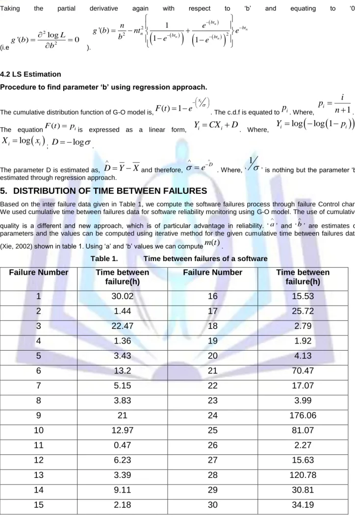
Based on the inter failure data given in Table 1, we compute the software failures process through failure Control chart. We used cumulative time between failures data for software reliability monitoring using G-O model. The use of cumulative quality is a different and new approach, which is of particular advantage in reliability. „
a‟ and „
b‟ are estimates of
parameters and the values can be computed using iterative method for the given cumulative time between failures data (Xie, 2002) shown in table 1. Using „a‟ and „b‟ values we can compute
m t
( )
.Table 1. Time between failures of a software
Failure Number
Time between
failure(h)
Failure Number
Time between
failure(h)
1
30.02
16
15.53
2
1.44
17
25.72
3
22.47
18
2.79
4
1.36
19
1.92
5
3.43
20
4.13
6
13.2
21
70.47
7
5.15
22
17.07
8
3.83
23
3.99
9
21
24
176.06
10
12.97
25
81.07
11
0.47
26
2.27
12
6.23
27
15.63
13
3.39
28
120.78
14
9.11
29
30.81
15
2.18
30
34.19
Assuming an acceptable probability of false alarm of 0.27%, the control limits can be obtained as (Xie, 2002):
0
.
99865
1
bt Ue
T
5
.
0
1
bt Ce
T
00135
.
0
1
bt Le
T
These limits are converted to
m t
( )
U ,m t
( )
C andm t
( )
L form. They are used to find whether the software process is incontrol or not by placing the points in Mean value chart shown in figure 1. A point below the control limit
m t
( )
L indicatesan alarming signal. A point above the control limit
m t
( )
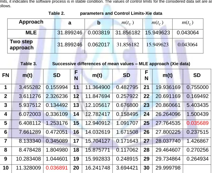
U indicates better quality. If the points are falling within the controllimits, it indicates the software process is in stable condition. The values of control limits for the considered data set are as follows.
Table 2. parameters and Control Limits-Xie data
Approach
a
b
m
(
t
U)
m
(
t
C)
m
(
t
L)
MLE
31.899246 0.003819 31.856182 15.949623
0.043064
Two step
approach
31.899246 0.062017
31.856182
15.949623
0.043064
Table 3. Successive differences of mean values – MLE approach (Xie data)FN
m(t)
SD
F
N
m(t)
SD
F
N
m(t)
SD
1
3.455282 0.155994
11
11.364900 0.482795
21
19.936169 0.755000
2
3.611276 2.326236
12
11.847694 0.257922
22
20.691169 0.169492
3
5.937512 0.134492
13
12.105617 0.676800
23
20.860661 5.403435
4
6.072003 0.336109
14
12.782417 0.158495
24
26.264096 1.500439
5
6.408112 1.253176
15
12.940912 1.091707
25
27.764535
0.035689
6
7.661289 0.472051
16
14.032619 1.671508
26
27.800225 0.237515
7
8.133340 0.345089
17
15.704127 0.171643
27
28.037740 1.426867
8
8.478428 1.804980
18
15.875771 0.117062
28
29.464607 0.270256
9
10.283408 1.044601
19
15.992833 0.248915
29
29.734864 0.264934
10
11.328009
0.036891
20
16.241748 3.694421
30
29.999798
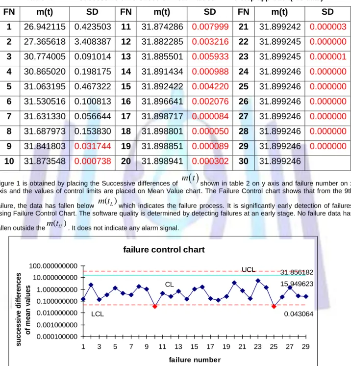
Table 4. Successive differences of mean values – Two step approach(Xie data)
FN
m(t)
SD
FN
m(t)
SD
FN
m(t)
SD
1
26.942115 0.423503
11
31.874286
0.007999
21
31.899242
0.000003
2
27.365618 3.408387
12
31.882285
0.003216
22
31.899245
0.000000
3
30.774005 0.091014
13
31.885501
0.005933
23
31.899245
0.000001
4
30.865020 0.198175
14
31.891434
0.000988
24
31.899246
0.000000
5
31.063195 0.467322
15
31.892422
0.004220
25
31.899246
0.000000
6
31.530516 0.100813
16
31.896641
0.002076
26
31.899246
0.000000
7
31.631330 0.056644
17
31.898717
0.000084
27
31.899246
0.000000
8
31.687973 0.153830
18
31.898801
0.000050
28
31.899246
0.000000
9
31.841803
0.031744
19
31.898851
0.000089
29
31.899246
0.000000
10
31.873548
0.000738
20
31.898941
0.000302
30
31.899246
Figure 1 is obtained by placing the Successive differences of
m t
shown in table 2 on y axis and failure number on x axis and the values of control limits are placed on Mean Value chart. The Failure Control chart shows that from the 9th failure, the data has fallen belowm t
( )
L which indicates the failure process. It is significantly early detection of failuresusing Failure Control Chart. The software quality is determined by detecting failures at an early stage. No failure data has fallen outside the
m t
( )
U . It does not indicate any alarm signal.Figure: 1 Failure Control Chart -MLE approach(Xie data)
failure control chart
UCL 31.856182 CL 15.949623 LCL 0.043064 0.000100000 0.001000000 0.010000000 0.100000000 1.000000000 10.000000000 100.000000000 1 3 5 7 9 11 13 15 17 19 21 23 25 27 29 failure number s uc c e s s iv e di ff e re nc e s of m e a n v a lue s
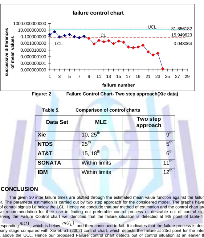
Figure: 2 Failure Control Chart- Two step approach(Xie data)
Table 5. Comparison of control charts
Data Set
MLE
Two step
approach
Xie
10, 25
th9
thNTDS
25
th5
thAT&T
15, 18
th6
thSONATA
Within limits
11
thIBM
Within limits
12
th6. CONCLUSION
The given 30 inter failure times are plotted through the estimated mean value function against the failure serial order. The parameter estimation is carried out by two step approach for the considered model. The graphs have shown out of control signals i.e below the LCL. Hence we conclude that our method of estimation and the control chart are giving a +ve recommendation for their use in finding out preferable control process or desirable out of control signal. By observing the Failure Control chart we identified that the failure situation is detected at 9th point of table-4 for the corresponding
m t
( )
, which is belowm t
( )
L and then continued to fail. It indicates that the failure process is detected atan early stage compared with Xie et. a1 (2002) control chart, which detects the failure at 23rd point for the inter failure data above the UCL. Hence our proposed Failure control chart detects out of control situation at an earlier than the situation in the time control chart. The early detection of software failure will improve the software Reliability. When the time between failures is less than LCL, it is likely that there are assignable causes leading to significant process deterioration and it should be investigated. On the other hand, when the time between failures has exceeded the UCL, there are probably reasons that have lead to significant improvement.
From Figure.2 the process is stabilized by touching the X-axis. Where as in Figure.1 there is a possibility of upward average number of failures also. As SPC is to stabilize at some point of time the two-step approach in Figure.2 is preferable.
7. REFERENCES
Kimura, M., Yamada, S., Osaki, S., 1995. ”Statistical Software reliability prediction and its applicability based on mean time between failures”. Mathematical and Computer Modeling Volume 22, Issues 10-12, Pages 149-155.
Koutras, M.V., Bersimis, S., Maravelakis,P.E., 2007. “Statistical process control using shewart control charts with supplementary Runs rules” Springer Science + Business media 9:207-224.
MacGregor, J.F., Kourti, T., 1995. “Statistical process control of multivariate processes”. Control Engineering Practice Volume 3, Issue 3, March 1995, Pages 403-414 .
failure control chart
UCL 31.856182 CL 15.949623 LCL 0.043064 0.000000000 0.000000001 0.000000100 0.000010000 0.001000000 0.100000000 10.000000000 1000.000000000 1 3 5 7 9 11 13 15 17 19 21 23 25 27 29 failure number s uc c e s s iv e di ff e re nc e s of m e a n v a lue s
Musa, J.D., Iannino, A., Okumoto, k., 1987. “Software Reliability: Measurement Prediction Application”. McGraw-Hill, New York.
Ohba, M., 1984. “Software reliability analysis model”. IBM J. Res. Develop. 28, 428-443.
Pham. H., 1993. “Software reliability assessment: Imperfect debugging and multiple failure types in software development”. EG&G-RAAM-10737; Idaho National Engineering Laboratory.
Pham. H., 2003. “Handbook Of Reliability Engineering”, Springer. Pham. H., 2006. “System software reliability”, Springer.
Gokhale, S.S and Trivedi, K.S., 1998. “Log-Logistic Software Reliability Growth Model”. The 3rd IEEE International Symposium on High-Assurance Systems Engineering. IEEE Computer Society.
Xie, M., Goh. T.N., Ranjan.P., (2002). “Some effective control chart procedures for reliability monitoring” -Reliability engineering and System Safety 77 143 -150.
Goel, A. L. and Okumoto, K., 1979, „Time-dependent error-detection rate model for software reliability and other performance measures‟, IEEE Transactions on Reliability, vol. 28, pp. 206-211.
Huang, C.Y and Kuo, S.Y., (2002). “Analysis of incorporating logistic testing effort function into software reliability modelling”, IEEE Transactions on Reliability, Vol.51, No. 3, pp. 261-270.
Kapur, P.K., Gupta, D., Gupta, A. And Jha, P.C., (2008). “Effect of Introduction of Fault and Imperfect Debugging on Release Time”, Ratio Mathematica, 18, pp. 62-90.
Krishna Mohan, G., Srinivasa Rao, B. and Satya Prasad, R. (2012). ”A Comparative study of Software Reliability models using SPC on ungrouped data”, International Journal of Advanced Research in Computer Science and Software Engineering. Volume 2, Issue 2, February.
Lewis-Beck, M., Bryman, A. and Futing, T. (Eds) (2003). “Least Squares”, Encyclopedia of Social Sciences Research Methods. Thousand Oaks (CA):Sage.
Liu, J., (2011). “Function based Nonlinear Least Squares and application to Jelinski-Moranda Software Reliability Model”, stat. ME, 25th August.
Lyu, M.R., (1996). “Handbook of Software Reliability Engineering”, McGraw-Hill, New York..
Xie, M., Yang, B. and Gaudoin, O. (2001). “Regression goodness-of-fit Test for Software Reliability Model Validation”, ISSRE and Chillarege Corp.