Contents lists available atScienceDirect
BioSystems
j o u r n a l h o m e p a g e :w w w . e l s e v i e r . c o m / l o c a t e / b i o s y s t e m s
Optimal parameter settings for information processing in gene regulatory
networks
Dominique F. Chu
a,∗, Nicolae Radu Zabet
a, Andrew N.W. Hone
b aSchool of Computing, University of Kent, CT2 7NF, Canterbury, UKbSchool of Mathematics, Statistics and Actuarial Science, University of Kent, CT2 7NF, Canterbury, UK
a r t i c l e i n f o
Article history:
Received 17 November 2010 Received in revised form 31 December 2010 Accepted 13 January 2011 Keywords:
Gene regulatory networks Noise
Speed Metabolic cost Trade-off
a b s t r a c t
Gene networks can often be interpreted as computational circuits. This article investigates the compu-tational properties of gene regulatory networks defined in terms of the speed and the accuracy of the output of a gene network. It will be shown that there is no single optimal set of parameters, but instead, there is a trade-off between speed and accuracy. Using the trade-off it will also be shown how systems with various parameters can be ranked with respect to their computational efficiency. Numerical analysis suggests that the trade-off can be improved when the output gene is repressing itself, even though the accuracy or the speed of the auto-regulated system may be worse than the unregulated system.
© 2011 Elsevier Ireland Ltd. All rights reserved.
1. Introduction
Living systems depend crucially on their ability to adjust to changes of both internal or external conditions or combina-tions thereof. Examples are seasonal changes, nutrient availability, encounters with predators, prey or mating partners and the like. Reacting to such changes requires the organism to perform com-putations. Higher animals have specialised nervous systems to this end. However, even within unicellular organisms, such as bacteria, there are computational processes going on at a molecular level. Individual proteins have been described as performing computa-tional functions (Bray, 1995). Another example of systems that can be considered as implementing computations are genes.
The idea that networks of genes can perform computational functions in the cell is now well established (seeFernando et al., 2009; Haynes et al., 2008; Ben-Hur and Siegelmann, 2004; Ziv et al., 2007). As a simple example consider the regulation of metabolic pathways in bacteria. The enzymes necessary to metabolize a spe-cific nutrient will only be activated if the nutrient is present in the environment (see for exampleChu et al., 2008), this metabolic con-trol implements a basic if-then statement. In this case a bacterial cell takes as input the concentration of an external nutrient con-centration, and “computes” an output, namely whether or not to turn on a metabolic pathway. This is probably the simplest
exam-∗Corresponding author.
E-mail address:D.F.Chu@kent.ac.uk(D.F. Chu).
ple of computing one could imagine. The next step in biological software sophistication is inducer exclusion (Narang, 2006; Narang and Pilyugin, 2007), i.e. the process whereby prokaryotic cells faced with several concurrently available nutrient sources exclusively take up the highest quality one. Beyond these examples, there are many more complicated instances of gene networks in cells where environmental information is integrated from a variety of sources to decide whether or not to turn on a gene (Mattick and Gagen, 2001).
The “computation” metaphor may not be useful in all contexts in theoretical biology, but in the case of gene networks it can be very enlightening. A network of genes that relays information from some input to some output can be parameterised in a number of ways. To see this consider the simplest model of the outputyof a single gene that is regulated by some molecule with concentration
x. This is a differential equation with a Hill functions as growth term:
˙
y=˛+ˇ x h
Kh+xh −yy.
Here˛andˇare the leak rate and the maximal growth rate respec-tively,handKare kinetic parameters of the Hill function, andx
is the concentration of the regulator molecule. Depending on the particular parameters of the system, the gene activation function will be a concave (h≤1) or sigmoid (h> 1) function of the concen-tration of the input molecules; the sensitivity of the function to a particular range of input concentrations depends onK;˛andˇ determine the output range of the gene. A gene network would be 0303-2647/$ – see front matter© 2011 Elsevier Ireland Ltd. All rights reserved.
modelled as a set of differential equations of the above type, where the network topology is determined by the dependencies between the equations.
For a cell, the particular choice of parameters is strongly con-strained by a number of factors: (i) The kinetic parameters of each gene must be such that each gene can be regulated over a physi-ologically relevant range of the inputx. Analogous considerations apply to the output range. (ii) The gene networks need to be able to process input sufficiently rapid, that is they need to change gene expression patterns, i.e. switch between steady states of protein concentrations, within a time that is appropriate given the bio-logical context of the genes. Within the computational metaphor this can be thought of as the computational speed of a gene net-work. (iii) The parameters’ impact on the metabolic cost must also be taken into account. Expressing proteins requires the cell to use ATP molecules; an expression rateˇof a gene comes at a contin-uous cost per time unit that is proportional toˇ. This presumably exerts a strong adaptive pressure on organisms that compete for limited resources. (iv) Proteins are discrete units expressed and degraded stochastically. This means that even at steady state con-centrations will be subject to random fluctuations (noise). Noise can be beneficial for the cell in some contexts, but is usually detri-mental when the function of a gene network is to relay/process information. The fluctuations around the signal make it harder for the cell to tell apart two signals that are close together, hence reducing the ability of a gene network to distinguish between sig-nals.
This uncertainty can be reduced if the cell averages the signals over a longer period of time. The intuition behind this is straight-forward: Assume a series of data points and assume further that it is known that these data points are distributed around a mean valuem1orm2. One can now ask how many data points need to be examined before one can, with a given level of confidence, decide between the two mean values. The answer is: It depends! More precisely it depends on the level of noise that affects the data and the distance betweenm1andm2. The closer they are together and the higher the noise the more sample points must be taken. Or, for a given level of noise, the more points are taken, the more confident one can be in determining the true mean value.
This is precisely the situation for a binary gene sensing its regulatory input. The more input data it collects, the more accu-rate the cell senses the activation state of the binary input, which implies that it will be more accurate in its output. However, col-lecting more input data takes time. What is more, mathematically it can be seen that it also entails that the gene switches slower between its two possible output levels. This manifests itself through a reduced computational speed of the gene. Hence, there is a trade-off between the accuracy of a cellular “computation” and its speed. This trade-off has been described n a recent contribution by Zabet and Chu (Zabet and Chu, 2009; Zabet et al., 2010), where it has been shown for the (near trivial) case of a single gene that noise and switching time cannot be separately optimised. They described a trade-off between the levels of noise of the output of a gene (which they call accuracy), the metabolic cost of expressing the gene, and the speed with which changes can be processed. For-mally, this manifests itself through the relationship of the switching time and the output noise with the decay rate of the output of the gene; these are proportional and inversely proportional, respec-tively.
The question of noise and speed of gene networks has previously received considerable attention in the community. In particular the impact of local network topologies, so-callednetwork motifs
(Oltvai and Barabasi, 2002; Milo et al., 2002a,b; Ma et al., 2009), on speed and noise has been researched in considerable detail. One of the results of this research is an emerging consensus that negative auto-regulation decreases the noise and switching time of a gene
(Alon, 2006, 2007; Singh and Hespanha, 2009; Wang et al., 2010; Bruggeman et al., 2009). However, many of the relevant studies on networks consider a limited range of parameters only. Moreover, they often do not keep the metabolic cost of sets of parameters they compare fixed. FollowingZabet and Chu (2009)this draws into question the comparison. Finally, most studies consider noise and switching speed separately, ignoring the trade-off between them.
Nearly all of the existing literature on stochastic fluctuations in gene networks focuses on noise at a particular steady state, in the sense that standard definitions of noise are normalised with respect to the steady state. This choice can be misleading when it is the aim to understand the computational limits of gene net-works. Processing and relaying signals requires that the individual components are able to adequately distinguish between different input signals. The classic model in computer science is to consider only two possible states per component, e.g. “on” or “off.” Trans-lated into the realm of gene networks this would mean that each gene can be either turned on (high expression/protein abundance) or turned off (low expression/protein abundance). Within such a binary model noise manifests itself through an uncertainty about the activation state of a gene. Depending on the size of the fluc-tuation and the difference between the high state and the low state (the signal strength) the cell needs to average out fluctu-ations by “repeat measurements.” The extent to which a given level of noise impairs the “distinguishability” of two signals does not primarily depend on the size of the fluctuations in relations to the steady state, but on the size of the fluctuations in relation to the difference between the two possible states, i.e. the sig-nal strength rather than by the steady state concentration. Hence, the appropriate measure of noise in this context is the size of the fluctuation normalised by the mean signal strength, as dis-cussed in the original article by Zabet and Chu. This seemingly minor modification, however, not only complicates the mathemat-ics considerably, but also alters the optimality properties of the system.
In this article, we will ask the same question asZabet and Chu (2009), but extend the analysis beyond their minimal network: Given a network of genes that is primarily computational in the above sense, what are the constraints on the choice of parameters? As it turns out, the answer to this question depends on the topology of the network. We therefore limit the scope of this article to net-works small enough to allow some exact analysis, thus striking a balance between feasibility and practical relevance. The hope is that the insights gained from this (if not the results themselves) gener-alize and create the right intuition for later large scale numerical simulation studies.
The main results presented here are as follows: We prove a num-ber of optimality properties of gene networks, including a lower bound on the noise of a gene network. Specifically, we show that the absolute fluctuations of negatively auto-regulated genes are always lower than those of comparable standard genes without negative auto-regulation, while this is no longer true when considering noise normalised by the signal strength. We also describe a methodology based on trade-off curves to compare two models of gene networks in terms of their computational efficiency. We could not find a sin-gle set of parameters for which negative auto-repression is inferior in terms of its computational properties.
2. Materials and Methods 2.1. The Model
In this article we consider three genes,Gx,GyandGz. The geneGyis regulated by an input signalxwhich we assume to change instantaneously from a high state xHto the low statexLorvice versa. Similarly,Gzis regulated by the product ofGy.
Gy Gz xH
xL Gy Gz
xH xL The output geneGzthus takes one of two possible steady state values depending
on the inputx.
We model gene expression as a one-step process, thus ignoring the noise con-tribution from mRNA expression (McAdams and Arkin, 1997; Paulsson, 2004; Raj and van Oudenaarden, 2008). The amount of translational noise depends crucially on the number of proteins produced from a single mRNA transcript and the lifetime of the mRNA transcript in relation to the protein product. While translational noise can be dominating, for most genes it is true that the overall noise is mainly driven by the underlying transcription dynamics (Bar-Even et al., 2006). In terms of the dependence of noise and time on the parameters of the system, this is therefore the main level to consider.
We denote the concentration of geneGzbyzand analogously forGy. In this article we will consider two regulation functions, the activator and the repres-sor. At steady state, if the input isxHthen the products of the genes take the valuesz* =zHandy* =yH, in the case of the activator andz* =zLandy* =yHin the case of the repressor. The asterisk indicates the steady state value of the relevant concentration. We model the dynamics of the system as a set of two differential equations: ˙ y=˛y+ωg(x)−yy ˙ z=˛z+ˇf(y)−zz (1) The symbols˛yand˛zrepresent the leak expression of the gene in the case of complete de-activation. Non-vanishing leak expression is probably common in biological systems, but is also a source of inefficiency of the system (seeZabet and Chu, 2009); since it does not add any interesting dynamical effects, we will assume
˛y=˛z= 0 throughout this contribution. Here the functionsgandfare assumed to be Hill functions given by:
g(x)= xh2
Kh2
2 +xh2
, f(y)= yh
Kh+yh
In the case of the repressor the Hill function is given by:
f(y)= Kh
Kh+yh
Note that we always assume the geneGyto be activated by its input. Following Zabet and Chu (2009)we define, the cost of the activator network, as the sum of the maximum production rates ofGyandGz:
=ωgH+ˇfH.
Here gH=˙g(xH); fH is defined analogously. In the case of the repressor we define the cost as =ωgL+ˇfH, to reflect that at steady state the genesGy andGz are never simultaneously activated. In order to keep the total cost of the gene network constant, we assume that the production rate ofzis given by
ˇ=−ωgH
fH
.
The system(1)can be solved analytically fory(t), but not for any subsequent gene products; however,z(t) can be given explicitly in terms of a quadrature, namely z(t)=e−zt
t 0 ezs˛ z+ˇf(y(s)) ds+C , (2)where the constantCdepends on initial conditions, and is zero if there is initially no product,z(0) = 0.
In the case of the negative auto-regulator (NAR), we model the system as follows:
˙
z=ˇfz(y)R(z)−zz (3)
where the negative auto-regulationRis given by
R(z)= K¯ ¯ h ¯ Kh¯+zh¯ and=˙R(zH)−1.
When assessing the relevance of stochastic fluctuations for sub-cellular infor-mation processing, the common definition of noise (variance divided by the mean or square of the mean (Paulsson, 2004; Ozbudak et al., 2002)) may not always be appro-priate. In essence, both of these measures relate the stochastic fluctuations at steady state to a (tacitly assumed) zero-concentration baseline. If defined in this way, noise is an indicator of the number of (statistically independent) measurements that are required in order to determine—within a given margin of error—the mean particle number in a cell. In many contexts this may be the relevant question to ask. In the context of information processing by genes it is not. If we assume binary genes, then
the absolute size of a signalS1may not be as important as the ability of the cell to distinguishS1from another signalS2in the presence of a given amount of stochastic fluctuations. This second signalS2may just be the absence of a signal, but this rarely works out to be a true zero baseline. Instead, “no signal” will typically mean “weak signal.”
Therefore, in order to assess the impact of the stochastic fluctuations on the computational properties of gene regulatory networks, it is necessary to modify this standard definition of noise. FollowingZabet and Chu (2009)we normalise the variance by the square of the signal strength (defined aszH−zL), rather than the signal itself, which is a measure of how the stochastic fluctuations limit an observer’s ability to distinguish one signal from another one. To compute the noise we use Paulsson’s version of van Kampen’s linear noise approximation (van Kampen, 2007; Paulsson, 2004). For the standard system this yields the formula
Nz= zH (zH−zL)2
intrinsic + regulation factor
ˇf H zH−zL z 2 time factor
y y+z 2 x extrinsic (4)
for the noise of z, while the noise formula for the NAR system evaluates to N= zH (1−fHRH− 1 z )(zH−zL)2 + 1 (zH−zL)2 (ˇf HRH)2 [ˇfHRH−z][−y+ˇfHRH−z] 2 y (5) Here we abbreviatedf(yH) byfH,df(yH)/dybyf Hand 1/zbyz.
We always evaluate the noise at the high state ofGz, because this state has the higher variance. The normalisation factorzH−zLis the same hence the noise at the high state will be higher, and is therefore chosen as the indicator for the noise of the system as a whole. Note that Eqs.(4) and (5)are the formulas for the activator. In the case ofGzbeing repressed byGythe termsfHandfH need to
be replaced byfLandfL. This is because the high statezHinGzis achieved when y* =yL.
2.2. Switching Time
In the language of dynamical systems that we use to model our system of genes, the computational speed of a system is determined by the time to switch from one state to another. In the simplest possible case of a binary sys-tem that we consider here, there are only two transitions, namely from/to a high state zH, and to/from a low statezL. Specifically, we interpret the time to switch as the time of the output to reach a fraction of one steady state (sayzH) given that the system starts in the other possible state (which would bezL in this case). In general, the transition timeTd
H
, from the high to the low state, and the time Tu
H
, from the low to the high states will not be equal, i.e.Tu(H)=/ Td(L). However, the maximum switching frequency is limited by T(), the slowest state transition time in the system, which is therefore a good indicator of the computational speed of a network of genes:
T()=max
Tu H , Td L , whereL=˙zH− (zH−zL) andH=˙zL+ (zH−zL).Here the subscriptsuanddabbreviate “up” and “down,” signifying whether the output signal is rising (Gzturning on) or fallingGz(turning off). The optimum configuration is reached where the time to switch the system on equals the time to switch it off, i.e.Tu(H) =Td(L).
2.3. Stochastic Model
We compared the noise prediction from the linear noise approximation with a Markov chain model corresponding to the deterministic system. The Markov chain model was constructed using the PRISM probabilistic model checker (Kwiatkowska et al., 2001), using the following code:
y : [miny..maxy] init miny;
z : [minz..maxz] init minz;
[]
(y <maxy) & (x>0)
-> omeg*(pow(x,h2)/(pow(x,h2) + pow(K2,h2))): (y’=y+1) ;
[]
(y> miny) -> y*m: (y’=y-1);
[]
(z <maxz) & (y>0)
-> beta*(pow(y,h)/(pow(y,h) + pow(K,h))): (z’=z+1) ;
[]
(z> minz) -> z*m: (z’=z-1);
To save space, we suppressed the specification of the parameters here. The noise was computed using two reward structures namely (i)true: z; and (ii) true: z*z;. The relevant property query was then given by:
((R{2}=? [ S ]-(R{1}=? [ S ])*(R{1}=? [ S ])))/pow(zh-zl,2)
PRISM can compute the exact numerical values (up to machine precision) of the noise; this approach is thus not only computationally more efficient than noise estimates based on stochastic simulations using Gillespie’s algorithm, but also more precise. The drawback of this approach is that it only works for relatively small models. In the present case, this works as long as the noise from the geneGxis considered negligible, which was the case inFig. 1(left). In the case of the positive auto-regulator inFig. 1(right)this was no longer the case and we had to resort to approximations of the noise by simulation. The model used in this figure had an additional stochastic variable x representing the particle number ofGxwith the following transition rates:
x : [minx..maxx] init minx;
[]
(y <maxx) & (x>0)-> 10: (x’=x+1) ;
[]
(x> minx) -> x*m: (x’=x-1);
Here we did not duplicate the items already listed above. 3. Results
In this section we report how the computational properties of the three-gene system depend on its parameters. In all cases we assume thatGyis activated byGxand we consider the cases where
Gzis activated/repressed byGyboth for the standard system and
the case ofGzrepressing its own expression.
3.1. Linear Chain without Feedback—The Standard System
For a linear chain of genes there are two distinct trade-offs between noise and time. Firstly, at a fixed metabolic cost the over-all noise of the output increases linearly with the decay rate (see equation(5) in SI 2), while the time to switch is inversely propor-tional to the decay rate (seeSI 4.2). This is a direct generalization of the noise-time trade-off that has been identified previously for a single gene (Zabet and Chu, 2009).
Secondly, there are optimal values of the Hill thresholdKfor noise and switching time. In general, these will not be equal. Hence, the values ofK in between the noise-optimum and the time-optimum realize a trade-off between noise and time, rep-resenting various possible combinations of noise and switching speed. In what follows, we describe these in more detail. For a fixed metabolic cost, decay rateand Hill thresholdK2 both the switching time and the noise have an optimal parameter value for the Hill threshold K of the gene Gz. Conversely, the
linear noise approximation predicts that for a fixed K there is an optimal valueK2 that minimizes the total noise of the out-put (see SI 3). When Gz is an activator, then as K→0 andK2 is kept optimal with respect to K, Eq.(4) predicts the noise to approach lim K→0N=
xh·h2 H xh·h2 L −xhH·h2 2 z . (6)Hence, the linear noise approximation does not predict an optimal value for the pair (K,K2) in the case of the activator. We expect
the linear noise approximation to become inaccurate for extreme parameter values, i.e. close toK= 0. An exact numerical analysis of the full Markov chain model shows that the linear noise approxi-mation holds well for even very lowKbut eventually breaks down before this minimum can be reached (seeFig. 1(left)).
The repressor case is somewhat different in that noise does not diverge for K→0, but approaches a finite value (see SI). Unlike the case of the activator, there is a global minimum for the noise in terms of the Hill coefficients K and K2, but it is not pos-sible to find a meaningful closed form solution for this global minimum.
Numerical analyses suggest that the time to switch is strongly dependent on the relative position ofKbetweenyHandyL.
Intu-itively, this can be understood as follows: In the case of an infinite Hill coefficienththe Hill thresholdKdefines the crucial limit for
ybelow which there is no activation and above which the gene is fully activated. Hence, if the Hill thresholdKis very low, then low levels ofywill fully activateGz, which entails thatGzwill be
acti-vated soon afterGxhas been activated. Hence, lowKmeans rapid
turn-on ofGz. Analogous reasoning applies when turning the
acti-vator off. The closer the Hill parameter to the activated stateyHthe
earlier the predecessor geneGyfalls to levels below the activation
threshold, and hence higher values ofKentail a faster switch-off. In the case ofh=∞we therefore find that the time-optimal value of the Hill threshold is given byK= (yH−yL)/2.
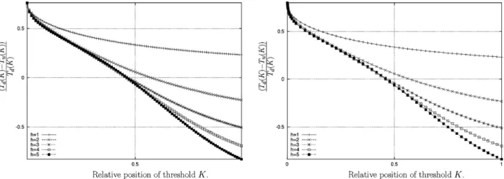
If we relax the assumption of an infinite Hill coefficient, the same qualitative reasoning still holds, but the optimumKwill not exactly coincide with the mid-point between the steady states ofGy.Fig. 1
illustrates the optimalKfor a number of numerical examples. The graph records a normalised difference between the time required to switch the gene off and the time required to switch it on, i.e. (Td(K)−Tu(K))/Td(K). The optimalKcoincides with the respective
times being equal, which is where the curves in the graph inter-sect the horizontal axis inFig. 1. The case of the repressor gene is analogous.
As stated previously (and inZabet and Chu, 2009), for each of the individual genesGyandGzthe computing time crucially depends
on the metabolic cost of the gene (assuming a fixed level of noise). In our present system the costs allocated to the individual genes can be altered as long as the boundary condition of a fixed total cost is respected, i.e.=ˇfH+ωgHremains constant. One could be tempted
to conjecture that the computing time will depend on how cost is allocated to the individual genes. We show inSI 5that this is not the case: The switching time is independent of the cost allocation. This rules out an allocation mediated trade-off between noise and time.
With respect to noise, the cost allocation does matter. In the limiting cases of all the cost being allocated to eitherGyorGzthe
noise goes to infinity which shows that there exists at least one minimum in between these extremes. It can also be shown that
Fig. 1.Switching on and off. (left) The horizontal axis is the relative position of the threshold parameter. The vertical axis represents the difference between the time required to switchGzon and off normalised by the time required to it switch on. The optimal parameter forKis where the line crossesx= 0. The various curves represent different Hill parametersh. The parameters used are as follows:ω= 2,h2= 2,xH= 5,xL= 0.1,= 4. The value of the decay rate was set to= 2 but note that each of the curves is invariant with respect to the decay rate. (right) Same as left but for the repressor.
any such minimum is independent of the decay rate, at least in the case of decay by dilution.
Fig. 2illustrates the noise-optimal cost distribution (and hence the optimalω) as a function of the relative strength of the upstream noise. It indicates a strong relationship between the amount of the upstream noise relative to the total noise and the cost allo-cation. Intuitively, this can be understood as follows: Allocating more resource toGyreduces the input noise toGzby increasing the
metabolic cost atGy, but at the expense of increasing the intrinsic
noise atGz. Depending on which noise source is the dominant one,
more or less cost should be allocated toGy. The same reasoning
holds in the case of the repressor, although the input noise tends to be low because it is generated by a low particle concentrationyL.
3.2. Negative Auto-regulation—The NAR System
Negative auto-regulation has been shown to attenuate noise and increase the switching time (Wang et al., 2010; Rosenfeld et al., 2002). Indeed, irrespective of its parameters, the variance of the
Fig. 2.Parametric plot of the optimal cost distribution (vertical) as a function of the ratio of the total noise to the input noise2
y(horizontal). The parameter varied
along the curve isK= [0. . .20]. The following parameters were used:ω= 2,h=h2= 2, xH= 5,xL= 0.1,= 4,K2= 0.04. The value of the decay rate was set to= 2 but note that each of the curves is invariant with respect to the decay rate and the cost.
NAR system is at worst equal to the noise of the corresponding standard system (seeSI). SectionSI 5shows that in the NAR system the variance is lowest for ¯K=0 and approaches the levels of the standard system forK=∞. This is true for both the repressor and the activator. However, it should be noted that this does not necessarily translate into a lower noise. The signalzH−zLin the NAR system is
at best as strong as in the standard system (seeSI 5). This means that there is the potential for the noise of the NAR system to be higher, even though the variance is lower. A full analytic treatment of the noise is hindered by the shape of the equation. In the case of the high state this is not a problem, becausezHis identical in the NAR system
and in the corresponding standard system. However, the steady state equation for the low statezLcannot be solved in general. We
are therefore largely limited to doing numerical analysis.
Fig. 3compares the noise of the NAR system and the standard system for some parameter values. The influence of ¯hseems to be more pronounced in the case of the NAR repressor than for the acti-vator. In both cases the Hill coefficient of the repression function does not seem to influence the noise qualitatively, in the sense that the range of parameters for which the standard system has bet-ter noise characbet-teristics is roughly unchanged. For a particular set of parameters,Fig. 3shows that the noise of the NAR activator is lower than the corresponding standard system. This contrasts with the case of the NAR repressor; the right hand side ofFig. 3 sug-gests that there is a significant proportion of the parameter space where the noise of the NAR repressor is higher than the correspond-ing standard system. Given that this is a particular example set of parameters, it is unclear to what extent this conclusion generalizes. Figs. 4 and 5 compare the switching times of the NAR and the standard system. A somewhat different picture presents itself. While with respect to noise the NAR activator seemed to have shown more benign computational properties throughout the parameter space, when it comes to the switching time there is a sizeable area where the NAR activator is slower than the standard system. This is specifically true for lower values of the Hill thresh-oldK, but the NAR activator is always faster onceKis sufficiently increased. There is also an area for very lowKwhere the NAR activa-tor is faster. However, this is unlikely to be of biological significance, because this corresponds toGzbeing only weakly controlled byGy.
The example also suggests that the Hill coefficient ¯hcorrelates neg-atively with speed once it is greater than 2, although the difference does not seem to be big. Lower Hill coefficients ¯hlead to NAR sys-tems that are overall more similar to the standard system. This is expected and for ¯h <1 this trend would continue. One can see from
Fig. 3.The noise of the NAR system (activator and repressor). (left) Comparing the noise of the NAR system with the standard system. The graph shows the ratio of the noise of the standard system and the NAR system for different Hill thresholds of the repressor function ¯K(x-axis) and Hill parameters ¯h. A value of 1 means that the systems have the same noise. A value <1 means that the standard system has higher noise. The parameters used are as follows:ω= 2,h= 3,h2= 2,xH= 5,xL= 0.1,= 4,= 1. The Hill constantsK2andKhave been kept at the midpoint between the high states ofxandy, respectively. (right) Same as left but for the NAR repressor.
Fig. 4.Comparing the switching time of the NAR (activator) system with the standard system. (left) The graph shows the ratio of the switching times of the NAR system and the standard system for different Hill coefficients of the NAR system ( ¯h). A value of 1 means that the systems have the same switching time. A value <1 means that the standard system is slower. The parameters used are as follows: ¯K=zH, ω=2, h=3, h2=2, xH=5, xL=0.1, =4, =1. (right) Same, but ¯h=2. The different plots
correspond to different relative positions of ¯K=z¯ H.
Fig. 6.Performance of the NAR system. (left) The-mediated noise-time trade-off of the standard system (solid line) compared to the NAR. The horizontal axis represents the switching timeTnar() and the vertical axis the noiseN. The parameters used are as follows:ω=2, h=3, h2=2,h¯=2, xH=5, xL=0.1, =4, K2=(1/2)xH, K=0.4yH.
(right) Same as left but for the repressor andK= 0.5yH.
the system of differential equations(3)that the regulation factor
Rreduces to 1 for ¯h=0 independent of ¯K; this means that in this limit the NAR system and the standard system are identical. The same is true for very large ¯K, when the contribution ofz(t) andzH
inR(z) andrespectively become negligible.
The example solutions shown inFig. 5indicate that the NAR repressor is faster than the standard system for most of the param-eters, i.e. only a small proportion of each graph reaches beyond 1. It is difficult to obtain analytical results for the switching time, although in the limiting case of ¯K=0 one can gain some insight. In this case the production rate in the differential equations is given byJ+=f
HzH/z(t). This can be integrated to obtain a general solution
corresponding to Eq.(2), namely
¯ z(T)=zH
(1+h¯) zH T 0 fet(1+h¯)dt+zH 1/(1+h¯) e−T (7)The trajectory of ¯z(t) can be seen to be the scaled version of an un-repressed system with a decay ratez=(1+h¯), whose solution
is denotedz(t). The trajectory from the high state to the low state can then be written as follows:
¯ z(T)=zH
z(T) zH 1+h¯1/(1+ ¯ h) . (8)Analogously, one can write the trajectory from the low state to the high state. The fact that the repressor is a scaled version of the un-repressed system, denoted byz(t), does not mean that ¯z(t) andz(t) have the same switching times. The reason is that the points ¯and where the respective systems reach a fraction of the distance between the high and the low state are not in direct correspon-dence. If we map the point ¯z(T¯)=¯ onto the corresponding point onz(t) then we obtain ¯ z(T¯)=
1− + z¯L zH 1/(1+h¯) .From Eq.(8)we can also calculate the low state of the system, that is ¯ zL=zH
z L zH 1/(1+h¯) . (9)The numerical examples so far show that the NAR system is sometimes noisier/slower than the standard system, this does not mean that the NAR system itself is “worse” than the standard system in terms of its computational properties.Fig. 6compares two trade-off curves. The trade-off curves of the NAR activator
are clearly below the standard system, which means that across the parameters varied the NAR systems has computationally more benign properties/trade-offs, and similarly in the case of the repres-sor. It should be noted that some of the points in the trade-off curves correspond exactly to points inFigs. 3 and 41: In the trade-off curves all points of the NAR system are below the standard system. At the same time, the activator corresponding to K= 0.4yHinFig. 4
is clearly slower than the corresponding standard system; simi-larly,Fig. 3shows that the noise of the NAR repressor is higher forK= 0.5yH. Nonetheless, for both of these parameters the
trade-off curve of the NAR system is below the standard system, which indicates an overall better computational performance than the corresponding standard system.
In order to get a better impression of the behavior of the system across the parameter space we performed a Monte-Carlo sampling of the parameter space. Fig. 7shows parameter sweeps for the behaviors of the NAR repressor and activator. Sampling different ωandKfurther corroborates the impression that there are signif-icant parts of parameter space where the NAR repressor is noisier than the standard system, and significant parts where the NAR activator is slower than the standard system. The interpretation of these parameter sweeps is aided by comparison with random points taken at optimalKon the rhs ofFig. 7. Two main obser-vations emerge from this. Firstly, the NAR repressor is both faster than the standard system and has lower noise when the Hill thresh-old parameter is optimised. Secondly, the activator has only lower noise, but is slower than the standard system at noise-optimalK.
Fig. 8shows a parameter sweep showing the time optimalK
for random parameters for the repressor. The result shows that for most points the NAR system is faster than the corresponding standard system.
4. Discussion
In order to survive, bio-systems need to perform computations on the state of their environment and their internal states. For bacteria one way to implement such computations are gene reg-ulatory networks. These can switch genes or sets of genes on and off depending on environmental or internal conditions or rather concentrations of molecular species that indicate such conditions.
1It is not possible to know from the graph precisely which points in the trade-off curve map to the corresponding points inFigs. 3 and 4, because the dots inFig. 6are not labeled with respect to the free parameter.
Fig. 7.Parameter sweep of the NAR system. (top) The graph shows noise-time trade-offs of the standard system compared to the NAR for both the positive regulator (lhs) and the negative regulator (rhs). This is a parametric plot ofNnar/Nstd. The variables that are varied are 0<K <¯ 2zHand 0.1≤ω≤4.1 each for ¯h=1,2,3,4,5. A
value below 1 on the horizontal and vertical axis respectively means that the noise/switching time of the NAR system is lower. The parameters used are as follows:
=1, ω=2, h=3, h2=2,h¯=2, xH=5, xL=0.1, =4, K2=(1/2)xH. (bottom) As top, but random parameter were chosen. For each set of parameters the optimal value
ofKwas calculated and used to generate the point. This graph is in log-scale for better readability.
Fig. 8.Parameter sweep of the NAR repressor system. As in the bottom right graph inFig. 7butKis optimised for switching time.
In this article we use a model of binary genes, that is each gene can be in one of two states only, “high” or “low.” This assumption signif-icantly simplifies the mathematics, but does not limit the generality of our conclusions. In genes that have more than two states, the same ideas as the one we present here apply. However, a detailed consideration of this case has to be left to future research.
We define a gene network as computing when it relays or pro-cesses changes of one and more input concentrations and regulates genes in response to this. In this article we exclusively consider binary genes, that is genes that have only two possible activa-tion states. In gene networks that are optimised for computing, there are two distinct trade-offs between the time to compute and the accuracy of the computation, a trade-off mediated by the decay rateand one mediated by the Hill thresholdsK. Mathe-matically, the former is the more fundamental one, in the sense that it is a consequence of how the noise and the switching time scale with the decay rate, namely (N∼) andT()∼1/, respec-tively. The biological interpretation of this-mediated trade-off is somewhat more difficult than the mathematics suggest. In bacterial cells, there is often no active break-down mechanism for proteins and concentrations diminish mainly through cell growth and divi-sion. Consequently, the decay rate will be related to the growth rate, which is time-varying and dependent on the nutrient supply.
Fig. 9. Optimality analysis and biological experiments. This figure shows theK-mediated noise time trade-off for the pR promoter as reported inRosenfeld et al. (2005). The trade-off is drawn in bold, and the sub-optimal points are in grey. We used the following set of parameters:V= 1.5×10⁻¹⁵l,
x==dilution= ln(2)/45 min−1, = 0.9,
˛= 0M min−1,xH= 0.006M andxL= 0.140M (Rosenfeld et al., 2005). The error bars were produced assuming an error of 20% forK±20 %. (left) Wild type as reported in Rosenfeld et al. (2005). (right) The mutant.
The growth rate and the availability of nutrients are only to a lim-ited extent free parameters of the cell. The-mediated noise-time trade-off is therefore best thought of as a physical constraint on the cell rather than the result of an evolutionary strategy.
In the case of active particle breakdown the interpretation is not much clearer. The issue is complicated by the fact that active breakdown requires at least one additional species of particles to break down or inactivate the primary regulator. This comes itself at an additional metabolic cost and thus complicates the analysis. Moreover, the presence of the breakdown particle does notper se
increase the switching speed because these breakdown particles need to be broken down themselves before a new signal can be built up. This may be circumvented by transporting particles to dedicated breakdown sites as it occurs in eukaryotic cells. Analyz-ing this case in terms of optimality considerations would go well beyond the scope of the present contribution.
Biologically, theKmediated trade-off is more rewarding to ana-lyze, at least in the context of prokaryotic gene regulation. The Hill thresholdKis related to the the binding and the un-binding rate constants of the transcription factor, and as such tunable over evolutionary time-scales. What makes the K-mediated trade-off interesting is that it provides insight into the adaptive pressures that shaped the parameters of the cell. When the parameters are known, then this can be used to understand what precisely the network is an adaptation to. When parameters arenotknown, then optimality considerations can be used to constrain the search space during parameter inference (e.g. during model fitting or via priors in Bayesian parameter estimation).
At present a problem are the high error rates which affect empir-ical estimates of kinetic parameters in gene regulatory networks. Fig. 9shows aK-mediated trade-off curve for thepRpromoter using parameters taken fromRosenfeld et al. (2005). They report errors for the value of the Hill threshold of about 20% and similarly high values for other parameters. Using the reported mean values, would locate the promoter just off the noise optimum; a mutant they reported in the same contribution would be just off the time opti-mum.Fig. 9also shows error bars around the points. We assumed that only the Hill threshold is affected by an error and that all the other parameters are certain. The figure shows that even in this overly optimistic scenario it is not possible to meaningfully locate individual genes on the trade-off curve. Note that a proper treat-ment of errors would also have to note an uncertainty around the
trade-off curve itself. Future more accurate information about the parameters will make this type of analysis more rewarding.
In order to analyze the noise-time trade-offs we used the van Kampen–Paulsson linear noise approximation. A comparison with exact calculations of the same Markov chain shows that the predic-tions of this approximation are very accurate for most parameters. However, there is still some caution warranted when interpret-ing the results with respect to real organisms. One source of error are the simplifying assumptions we made in order to arrive at the dynamical model of the gene networks (i.e. Eqs.(1) and (3)).
One of these assumptions concerns the input (i.e. the product of the geneGx) which we assumed to be flipping instantaneously
between the high statexHand the low statexL, a condition that
is clearly never fulfilled in nature. However, we have mainly con-centrated on qualitative aspects of the dynamics, that is how observable features of the gene network depend on the parameters of the system and we are not trying to present a predictive model of a specific system. Relaxing the assumption of instantaneous input will not affect the qualitative relations we have established; the assumption is therefore of little consequence to our conclusions.
Another aspect that is clearly not taken into account in our model is the time delay due to the translation step which, amongst other things, will depend on the length of the protein. The length of the protein will also enter into the cost function thus complicat-ing the analysis. For our current purposes these are second order effects that will be important in quantitative models of specific sys-tems, but are of minor relevance for the conceptual understanding we are trying to develop here.
Of more direct impact for our models is the breakdown of the lin-ear noise approximation for extreme parameters. The FDT approach predicts that there is a theoretical minimal value for the noise given by Eq.(6); this can be reached in the limit of a vanishingK(while keeping K2 optimal).Fig. SI 1(left)indicates that the theoretical estimates for the noise become inaccurate for very low values ofK
which means that this global optimum will probably not be repro-duced by real systems even though (at least for the parameters in the graph) the linear noise approximation is a good indicator for a wide range of parameters (seeFig. SI 2 and SI 1(left)). Add to this that the model itself is a simplification and we must conclude that the prediction of Eq.(6)may be far from biological reality in quan-titative terms. On the other hand, the linear noise approximation
has successfully been applied to real biological systems and it is therefore reasonable to assume that the overall qualitative picture it paints is relevant.
In the literature, there is a general consensus developing that self-repressing genes have more benign noise and time (Rosenfeld et al., 2002; Wang et al., 2010) properties than a standard gene with the same parameters. Indeed, in bacteria estimates for the proportion of NAR genes among all genes range from 40 to 60% (Rosenfeld et al., 2002; Alon, 2007). However, there is no obvious metabolic cost in negative auto-regulation, which begs the ques-tion why not all genes are auto-repressors. Part of the answer is that the idea of gene networks as computing input is not always true. Sometimes genes fulfill functions other than information pro-cessing. In those the main adaptive pressures may not come from noise and/or switching speed, but from other considerations. There may be systems that need to switch fast in one direction only. In this case the trade-off curves would have to be drawn very dif-ferently, thus altering the conclusions reached here. Finally, in our analysis we did not consider motifs other than the standard system and negative auto-regulation. For example, in some circumstances Feed-Forward Loop network motifs (Mangan and Alon, 2003) may be more suitable than negative auto-regulation.
The linear noise approximation predicts that the variance is always lower in the NAR system than in the standard system. This entails that the noise, if taken against a zero-concentration baseline is lower. However, if the baseline signal corresponds to a non-vanishing concentration, then the noise of the NAR system may be higher than in the standard system. In the case of the NAR repressor we even found this to be the typical behavior for the range of param-eters we considered. On the other hand, our Monte-Carlo parameter sweeps indicate that the NAR-activator is typically less noisy than the corresponding standard system, although there are significant parts of parameter space where the auto-regulated system is slower than the standard system.
Biologically the typical behavior of a system may not be as rele-vant as the optimal behavior to which adaptive pressures drove the system. This is particularly true in the present case where the typical behavior of the system is very different from the opti-mal behavior: Both at its noise-optiopti-malKand its time-optimalK
the repressor is faster and less noisy than the standard system (seeFigs. 7 and 8). In the case of the activator the case is not as clear cut. For all but a few example parameters we generated, at noise-optimalKthe NAR system has lower noise than the standard system, but the switching time is higher.
From our analysis it is clear that the computational efficiency of gene networks cannot be indicated by a single variable only, but must be assessed across the parameter space using trade-off curves. While we found that sometimes the negative regulator has indeed higher noise than the corresponding standard system, we could not find a single example where the NAR system did not lead to an overall better noise-time trade-off than the corresponding stan-dard system. This leads us to the conclusion that the NAR system has a better computational performance than the standard system. More generally, however, this suggests that trade-off curves can be very useful tool when exploring optimal parameter ranges for bio-systems.
Appendix A. Supplementary data
Supplementary data associated with this article can be found, in the online version, atdoi:10.1016/j.biosystems.2011.01.006. References
Alon, U., 2006. An Introduction to Systems Biology: Design Principles of Biological Circuits. Chapman & Hall.
Alon, U., 2007. Network motifs: theory and experimental approaches. Nature Review Genetics 8 (June (6)), 450–461,http://dx.doi.org/10.1038/nrg2102.
Bar-Even, A., Paulsson, J., Maheshri, N., Carmi, M., O’Shea, E., Pilpel, Y., Barkai, N., 2006. Noise in protein expression scales with natural protein abundance. Nature Genetics 38 (June (6)), 636–643,http://dx.doi.org/10.1038/ng1807.
Ben-Hur, A., Siegelmann, H., 2004. Computation in gene networks. Chaos 14 (March (1)), 145–151,http://dx.doi.org/10.1063/1.1633371.
Bray, D., 1995. Protein molecules as computational elements in living cells. Nature 376, 307–313.
Bruggeman, F., Bluethgen, N., Westerhoff, H., 2009. Noise management by molec-ular networks. PLoS Computational Biology 5 (September (9)), e1000506, http://dx.doi.org/10.1371/journal.pcbi.1000506.
Chu, D., Roobol, J., Blomfield, I., 2008. A theoretical interpretation of the transient sialic acid toxicity of ananRmutant ofEscherichia coli. Journal of Molecular Biology 375, 875–889.
Fernando, C., Liekens, A., Bingle, L., Beck, C., Lenser, T., Stekel, D., Rowe, J., 2009. Molecular circuits for associative learning in single-celled organisms. Journal of the Royal Society Interface 6 (May (34)), 463–469,http://dx.doi. org/10.1098/rsif.2008.0344.
Haynes, K., Broderick, M., Brown, A., Butner, T., Dickson, J., Harde, W., Heard, L., Jessen, E., Malloy, K., Ogden, B., Rosemond, S., Simpson, S., Zwack, E., Campbell, A., Eckdahl, T., Heyer, L., Poet, J., 2008. Engineering bacteria to solve the burnt pan-cake problem. Journal of Biological Engineering 2 (1), 8,http://www.jbioleng. org/content/2/1/8.
Kwiatkowska, M., Norman, G., Parker, D., 2001. PRISM: Probabilistic symbolic model checker. In: Kemper, P. (Ed.), Proc. Tools Session of Aachen 2001 International Multiconference on Measurement, Modelling and Evaluation of Computer-Communication Systems, pp. 7–12, available as Technical Report 760/2001, University of Dortmund, September.
Ma, W., Trusina, A., El-Samad, H., Lim, W.A., Tang, C., 2009. Defining network topolo-gies that can achieve biochemical adaptation. Cell 138 (4), 760–773. Mangan, S., Alon, U., 2003. Structure and function of the feed-forward loop
network motif. Proceedings of the National Academy of Sciences of the United States of America 100 (October (21)), 11980–11985,http://dx.doi.org/ 10.1073/pnas.2133841100.
Mattick, J., Gagen, M., 2001. The evolution of controlled multitasked gene networks: the role of introns and other noncoding rnas in the development of complex organisms. Molecular Biology and Evolution 18 (September (9)), 1611–1630. McAdams, H., Arkin, A., 1997. Stochastic mechanisms in gene expression.
Proceed-ings of the National Academy of Sciences of the United States of America 94 (February (3)), 814–819.
Milo, R., Shen-Orr, S., Itzkovitz, S., Kashtan, N., Chklovskii, S., Alon, U., 2002a. Net-work motifs in the transcriptional regulation netNet-work ofEscherichia coli. Nature Genetics 31, 64–68.
Milo, R., Shen-Orr, S., Itzkovitz, S., Kashtan, N., Chklovskii, S., Alon, U., 2002b. Network motifs: simple building blocks of complex networks. Science 298, 824–827.
Narang, A., 2006. Comparative analysis of some models of gene regulation in mixed-substrate microbial growth. Journal of Theoretical Biology 242 (September (2)), 489–501.
Narang, A., Pilyugin, S., 2007. Bacterial gene regulation in diauxic and non-diauxic growth. Journal of Theoretical Biology 244 (January (2)), 326–348, http://dx.doi.org/10.1016/j.jtbi.2006.08.007.
Oltvai, Z., Barabasi, A., 2002. Life’s complexity pyramid. Science 298, 763–764. Ozbudak, E., Thattai, M., Kurtser, I., Grossman, A., van Oudenaarden, A., 2002.
Regu-lation of noise in the expression of a single gene. Nature Genetics 31 (May (1)), 69–73,http://dx.doi.org/10.1038/ng869.
Paulsson, J., 2004. Summing up the noise in gene networks. Nature 427 (January (6973)), 415–418,http://dx.doi.org/10.1038/nature02257.
Raj, A., van Oudenaarden, A., 2008. Nature, nurture, or chance: stochastic gene expression and its consequences. Cell 135 (October (2)), 216–226, http://dx.doi.org/10.1016/j.cell.2008.09.050.
Rosenfeld, N., Elowitz, M., Alon, U., 2002. Negative autoregulation speeds the response times of transcription networks. Journal of Molecular Biology 323 (November (5)), 785–793.
Rosenfeld, N., Young, J., Alon, U., Swain, P., Elowitz, M., 2005. Gene reg-ulation at the single-cell level. Science 307 (March (5717)), 1962–1965, http://dx.doi.org/10.1126/science.1106914.
Singh, A., Hespanha, J., 2009. Optimal feedback strength for noise suppression in auto-regulatory gene networks. Biophysical Journal 96 (May (10)), 4013–4023. van Kampen, N., 2007. Stochastic Processes in Physics and Chemistry, third edition.
Elsevier, Amsterdam.
Wang, L., Xin, J., Nie, Q., 2010. A critical quantity for noise attenua-tion in feedback systems. PLoS Computaattenua-tional Biology 6 (4), e1000764, http://dx.doi.org/10.1371/journal.pcbi.1000764.
Zabet, N., Chu, D., 2009. Computational limits to binary genes. Journal of the Royal Society Interface, 10,http://www.cs.kent.ac.uk/pubs/2009/2969, December. Zabet, N., Hone, A., Chu, D., 2010. Design principles of transcriptional logic circuits.
In: Artificial Life XII Proceedings of the Twelfth International Conference on the Synthesis and Simulation of Living Systems ,. MIT Press, August, pp. 186–193, http://www.cs.kent.ac.uk/pubs/2010/3036.
Ziv, E., Nemenman, I., Wiggins, C., 2007. Optimal signal processing in small stochastic biochemical networks. PLoS One 2 (10), e1077,http://dx.doi.org/10. 1371/journal.pone.0001077.