issn0899-1499|eissn1526-5528|00|0000|0001 c0000 INFORMS
A branch-and-price algorithm for parallel machine
scheduling using ZDDs and generic branching
Daniel Kowalczyk, Roel Leus
ORSTAT, Faculty of Economics and Business, KU Leuven, Naamsestraat 69, 3000 Leuven, Belgium [email protected], [email protected]
We study the parallel machine scheduling problem to minimize the sum of the weighted completion times of the jobs to be scheduled (problem P m||P
wjCj in the standard three-field notation). We use the set
covering formulation that was introduced by van den Akker et al. (1999) for this problem, and we improve the computational performance of their branch-and-price (B&P) algorithm by a number of techniques, including a different generic branching scheme, zero-suppressed binary decision diagrams (ZDDs) to solve the pricing problem, dual-price smoothing as a stabilization method, and Farkas pricing to handle infeasibilities. We report computational results that show the effectiveness of the algorithmic enhancements, which depends on the characteristics of the instances. To the best of our knowledge, we are also the first to use ZDDs to solve the pricing problem in a B&P algorithm for a scheduling problem.
Key words: parallel machine scheduling, weighted completion times, branch and price, ZDD, stabilization
1.
Introduction
In this paper we report on our improvements to the branch-and-price (B&P) algorithm of van den Akker et al. (1999) for the parallel machine scheduling problem with weighted completion-time objective on identical machines, which is written as P m||P
wjCj in the
standard three-field notation. For brevity we refer to the problem as WCT. A B&P algo-rithm is a branch-and-bound (B&B) algoalgo-rithm in which at every node of the B&B tree a lower bound is computed via a linear-programming (LP) relaxation with a large number of variables. The LP relaxation, called the master problem, is solved using column genera-tion (CG). B&P algorithms are used in many areas of operagenera-tions research, such as vehicle routing (Agarwal et al., 1989; Fukasawa et al., 2006), vertex coloring (Mehrotra and Trick, 1996), bin packing and cutting stock problem (Vance et al., 1994), etc. In a given node of the search tree, the master problem only contains a restricted number of promising vari-ables and is called therestricted master problem (RMP). The RMP is solved with standard
LP techniques. It can, but need not, yield an optimal solution to the full master problem with all columns included. The search for a new column with negative reduced cost to be included in RMP is called the pricing problem, which is an optimization problem that depends on the definition of the variables, and which has a non-linear objective function in our case. In van den Akker et al. (1999) the authors solve the pricing problem using a gen-eral dynamic-programming (DP) recursion. In our work, we use a zero-suppressed binary decision diagram (ZDD) to do this, which is a data structure that represents a family of sets. Concretely, a ZDD is constructed as a directed acyclic graph (DAG) such that each machine schedule corresponds with a path from the root node of the DAG to one partic-ular leaf node, which will allow to find a schedule with minimum (negative) reduced cost. Solving pricing problems with the help of ZDDs was first done in Morrison et al. (2016b), who show how to adjust the ZDD when a standard integer branching scheme is applied for vertex coloring (when fractional variable λ equals α, then two children are created with additional constraints λ≤ bαc and λ≥ dαe). With standard integer branching, the structure of the pricing problem is typically destroyed, and so van den Akker et al. (1999) devise a specialized branching scheme that allows to re-use the same pricing algorithm in every node of the B&B tree. In this paper we explain how to adapt the ZDD when the generic branching scheme of Ryan and Foster (1981) is used, which will have a clear impact on the convergence of the B&P algorithm, meaning that the algorithm will explore fewer nodes in the search tree.
Another improvement that we include in the B&P algorithm is the use of stabilization techniques for CG. It is well known that CG methods for machine scheduling suffer from poor convergence because of extreme primal degeneracy and alternative dual solutions. These phenomena have a large impact especially when the number of jobs per machine is high. One of these techniques is dual-price smoothing, which was introduced in Wentges (1997). This technique corrects the optimal solution of the dual problem of the restricted LP relaxation based on past information before it is plugged into the pricing algorithm. This stabilization is very important for calculating the lower bound, but identifying upper bounds is obviously also of vital importance. In our computational experiments we will see that the branching scheme of van den Akker et al. (1999) performs rather poorly on some instance classes, even when stabilization is applied, and then the choice of the branching
scheme matters. As pointed out by Morrison et al. (2016b), using ZDDs for pricing gives the possibility to implement a generic B&P algorithm.
The remainder of this paper is structured as follows. In Section 2 we first provide a formal problem statement and a number of pointers to the existing literature. Subsequently, in Section 3 we list some characteristics of optimal solutions and describe an integer linear formulation. The formulation is solved by means of B&P, the main aspects of which are explained in Section 4. Section 5 then provides more information on ZDDs in general, and on the way in which we use ZDDs to solve the pricing problem. More details on Farkas pricing as a way to handle infeasibilities, on stabilization and on the branching strategy are given in Sections 6, 7 and 8, respectively. The main findings of our computational experiments are discussed in Section 9, and we conclude the paper in Section 10.
2.
Problem definition and literature overview
We consider a set J ={1, . . . , n} of n independent jobs with associated processing times pj∈N0 for j ∈J, which need to be processed on a set M ={1, . . . , m} of m identical
machines. Each machine can process at most one job at a time and preemption is not allowed. The objective of problem WCT is to find an assignment of the jobs to the machines and to decide the sequencing of the jobs on the machines such that the objective function
Pn
j=1wjCj is minimized, where wj ∈N0 is the weight of job j ∈J and Cj the completion
time. This problem is N P-hard for m≥2, see for instance Bruno et al. (1974) or Lenstra et al. (1977). We assume that n > m in order to avoid trivialities. Case m= 1 (only one machine) is known to be solvable in polynomial time, because one can show that there exists an optimal schedule with the following two properties:
Property 1. The jobs are sequenced following Smith’s shortest weighted processing-time
(SWPT) rule (Smith, 1956), which orders the jobsj in non-increasing order of the ratio wjpj.
Property 2. The jobs are processed contiguously from time zero onward.
Since the machines can be considered independently of each other after the assignment of the jobs to machines, an optimal solution exists for WCT that has the same properties; the difficulty of the problem therefore resides in the job-machine assignment. Several DP approaches have been proposed for WCT that exploit this idea. These algorithms run in O(n(P
j∈Jpj) m−1
) time (Rothkopf, 1966; Lawler and Moore, 1969), or inO(n(P
j∈Jwj) m−1
time (Lee and Uzsoy, 1992). Consequently, these algorithms become unmanageable when the number of machines, the processing times or the weights increase.
In the literature, B&P methods have been proposed that exploit Properties 1 and 2. Chen and Powell (1999) and van den Akker et al. (1999) devise an algorithm with CG-based lower bound resulting from a partition formulation of WCT, where a variable corresponds to a single machine schedule with a specific structure (see Section 3). The algorithms differ in their branching scheme, as well as in the pricing algorithm (although both are DP-based). It should be noted that the lower bounds are very tight.
B&P approaches for parallel machine scheduling do not always exploit Property 1, or another optimal ordering rule. Dyer and Wolsey (1990) introduce a time-indexed formu-lation for a problem with a general time-dependent objective function. The number of variables is O(nT), whereT depends on the processing times. This type of formulation has very good bounds but cannot be applied directly because of the pseudo-polynomial number of variables and constraints. This problem is partially mitigated in van den Akker et al. (2000) by applying Dantzig-Wolfe decomposition, and then CG is used for computing the lower bound. The pricing problem is a shortest path problem on a network of size O(nT). Branching can be applied on the original variables of the time-indexed formulation without much effort, i.e., the pricing algorithm stays the same, only the network in which a shortest path is calculated changes.
Another model is the arc-time-indexed formulation proposed by Pessoa et al. (2010), where a binary variable zijt is defined for every pair of jobs (i, j) and every period t such
that zijt = 1 if job i finishes and job j starts at t. The resulting formulation is huge,
but also has some advantages over the time-indexed model. Dantzig-Wolfe decomposition is then applied to obtain a reformulation with an exponential number of variables, each corresponding to a path in a suitable network. The running time of the pricing algorithm is O(n2T). Pessoa et al. (2010) recognize that stabilization techniques are important to
quickly compute the lower bound and overcome the convergence issue for this type of formulation.
Other techniques to resolve the slow convergence of B&P for time-indexed formula-tions have been proposed by Bigras et al. (2008), who use temporal decomposition, and by Sadykov and Vanderbeck (2013), who put forward the technique of column-and-row generation together with stabilization. Note that, depending on the instance, the duality
gap for these formulations may be difficult to close, and so the B&B tree can still be very large. Recently, B¨ulb¨ul and S¸en (2017) have also introduced another novel formulation for minimizing the total weighted completion time on unrelated machines, which is solved with a Benders decomposition technique and which has a limited gap.
3.
Structure of optimal solutions and linear formulation
We assume that the jobs are indexed in non-increasing order of the ratio wjpj, i.e.,
w1
p1 ≥ · · · ≥ wn
pn, so that Property 1 is easily invoked for each machine separately. Denote
by p[i] the [i]-th smallest processing time among the jobs in J, and let pmax=p[n] be the
largest value among all pj. We can now state some further properties of optimal solutions
to WCT, with Sj the starting time of job j:
Property 3 (Belouadah and Potts, 1994). There exists an optimal solution for
which the latest completion time on any machine is not greater than Hmax=
P
j∈Jpj
m +
m−1 m pmax.
Property 4 (Azizoglu and Kirca, 1999). There exists an optimal solution for
which the latest completion time on any machine is not less than Hmin = 1 m P j∈Jpj− Pm−1 h=1 p[n−h+1] .
Property 5 (Elmaghraby and Park, 1974). Sj1 ≤Sj2 in an optimal solution if one
of the following conditions holds:
• pj1< pj2 and wj1 ≥wj2, or • pj1≤pj2 and wj1 > wj2.
Property 6 (Azizoglu and Kirca, 1999). Sj1 ≤Sj2 in an optimal solution if j1−1 X h=1 ph≤ 1 m X j∈J pj− m−1 X h=1 p[n−h+1] ! − n X h=j2 ph.
These properties have consequences for the execution intervals of the jobs. The execution interval of jobj is described by a release daterj, before which the job cannot be started, and
a deadlinedj, by which the job has to be completed. By Property 3 we can set rj= 0 and
dj=Hmax for every j∈J. In van den Akker et al. (1999) the authors use only Property 5
to deduce tighter release dates and deadlines for every job. In this text we will also use Property 6; this can have a great influence on the tightness of the time windows.
Define the following subsets of jobs for each j∈J: Pj1={k∈J|(wk> wj∧pk≤pj)∨(wk≥wj∧pk< pj)} (1) and P2 j = ( k∈J k < j and k−1 X h=1 ph≤ 1 m n X h=1 ph+ m−1 X h=1 p[n−h+1] ! − n X h=j ph ) . (2) LetPj be the union ofPj1 andPj2. Because of Properties 5 and 6 we know that there exists
an optimal solution in which all jobs ofPj start no later than job j. Hence if|Pj|> m−1,
then we know that there are at least |Pj| −m+ 1 jobs that should be completed before
job j is started. Denote by ρj the sum of the durations of the |Pj| −m+ 1 jobs inPj with
smallest processing time, then we can setrj= ρj
m
. The derivation of tighter deadlines can proceed similarly: define
Q1 j={k∈J|(wk< wj∧pk≥pj)∨(wk≤wj∧pk> pj)} (3) and Q2 j = ( k∈J k > j and j−1 X h=1 ph≤ 1 m n X h=1 ph+ m−1 X h=1 p[n−h+1] ! − n X h=k ph ) . (4) Let Qj be the union of Q1j and Q2j. Similarly as before, there exists an optimal solution
for which Sj ≤Sj0 for every j0 ∈ Qj, so the amount of work that has to be done between
Sj and Hmax is equal to Pj0∈Q
jpj0+pj. Consequently, job j cannot start later than δj=
Hmax− l P j0∈Q jpj 0+pj
/mm, and if δj+pj< dj then we updatedj to value δj+pj.
Below we describe an integer linear formulation for WCT. Every binary variable λs
corresponds to an assignment of a subset s⊂J of jobs to one machine, with which we can associate a unique schedule viaCj(s) =Pi∈s:i≤jpi for each j∈s. We only consider job
sets s that respect the execution intervals corresponding to the ready times and deadlines that where established above. Concretely, let S be the set of all sets s⊂J that lead to a feasible schedule, meaning that rj+pj≤Cj(s)≤dj for all j∈s, and that the completion
time of the last job included ins is betweenHmin andHmax. We should note that van den
Akker et al. (1999) use a weaker form of Property 4 for computingHmin. In the formulation
below we represent such schedules by binary vectors of dimension n. Every schedule s has an associated cost cs= X j∈s wj X k∈s:k≤j pk ! . (5)
We now need to find m schedules of S such that every job j∈J is chosen and the total weighted completion time is minimized. This can be cast into the following set covering formulation: minimize X s∈S csλs (6a) subject to X s∈S:j∈s λs≥1 for each j∈J (6b) X s∈S λs≤m (6c) λs∈ {0,1} for each s∈ S (6d)
This formulation has n covering (assignment) constraints and one capacity constraint. Condition (6b) ensures that every jobj is assigned to one machine, constraints (6c) impose that we use only mmachines, and constraints (6d) state that the variables are all binary. Although it might be more intuitive to write equality in (6b) and (6c), resulting in a partition formulation, our experimental results indicate that the covering formulation performs better than the partition formulation in the LP relaxation phase. The reason is that the dual variables corresponding to the equality sign in the constraints (6b) and (6c) of the LP relaxation of the partition formulation are less constrained. The LP relaxation of the set covering formulation has faster convergence and is more stable than the relaxation of the partition formulation. Similar observations are reported in Lopes and de Carvalho (2007).
4.
A B&P algorithm for WCT
Formulation (6) has an exponential number of variables. Listing all the schedules of S
would be impractical and we will therefore devise a B&P algorithm. The main differences between the algorithm of van den Akker et al. (1999) and our implementation are the following:
1. We use a generic branching scheme that was introduced by Ryan and Foster (1981) for partitioning formulations. In van den Akker et al. (1999) the authors develop a problem-specific branching scheme that does not destroy the structure of the pricing problem.
2. Since our branching scheme does affect the structure of the pricing problem in the root node, we develop a different pricing algorithm that is based on ZDDs. The details of this pricing routine are described in Section 5. To the best of our knowledge, we are the first to use ZDDs to solve the pricing problem in a B&P algorithm for a scheduling problem.
3. When a new branching decision is made in the search tree, it is possible that the RMPs in the newly created child nodes are infeasible. We handle such infeasibility by applying Farkas pricing; we refer to Section 6 for more details.
4. We also use a stabilization technique in order to manage several drawbacks inherent in the use of CG; see Section 7. This will be very important for calculating the lower bound in the root node, in particular for instances with many jobs per machine. We first seek to solve the LP relaxation of (6), which corresponds with the objective function (6a), the constraints (6b) and (6c), and
λs≥0 for eachs∈ S (7)
The dual of this LP relaxation is given by: maximize X j∈J πj−mσ (8a) subject to X j∈s πj−σ≤cs for each s∈ S (8b) πj≥0 for each j∈J (8c) σ≥0 (8d)
where values πj for j∈J are the dual variables associated to constraints (6b) andσ is the
dual variable associated to constraint (6c). The constraints (8b) derive from the primal variablesλ. The LP relaxation is solved by CG, so we iteratively solve a RMP instead of the full relaxation and check whether there exists a column that can be added to improve the current optimal solution, which is done in the pricing problem. The columns are schedules from a restricted setSr⊂ S. At each iteration we check whether constraint (8b) is violated,
and if so then we add the corresponding primal variable. The termination conditions for this CG procedure depend on the stabilization technique, and will be explained in Section 7.
The pricing problem is the following: ifπj∗ forj∈J andσ∗ represent the current optimal solution of the dual of the RMP, then does there exist a schedules∈ S for whichP
j∈sπ
∗
σ∗> cs? The LP relaxation is typically solved faster if we first add constraints that are
strongly violated, and we will search for schedules with most negative reduced cost. This can be modeled as follows:
minimizecs− X
j∈s
πj∗ (9a)
subject to s∈ S, (9b)
becauseσ∗ is independent ofS. Note thatcs in the objective function (9a) is quadratic (see
Equation (5)). This pricing problem is solved by DP in van den Akker et al. (1999). Their forward recursion uses the insight from Property 1 that each machine schedule can follow the SWPT rule. The DP-based algorithm runs in O(nHmax) time. In the next section, we
will show how ZDDs can be used in a pricing algorithm.
5.
Zero-suppressed binary decision diagrams for the pricing problem
5.1. General introduction to ZDDs
Zero-suppressed binary decision diagrams (ZDDs) are data structures that allow to rep-resent and manipulate families of sets that can be linearly ordered in a useful manner. They were proposed by Minato (1993) as extensions of binary decision diagrams (BDDs). BDDs were introduced by Lee (1959) and Akers (1978) as DAGs that can be obtained by reducing binary decision trees that represent the decision process through a set of binary variables of a Boolean function. A ZDDZ is a DAG that has two terminal nodes, which are called the 1-node and 0-node. Every nonterminal node i is associated to an element v(i) (the label of node i) of a set and has two outgoing edges: the high edge, which points to the high child node hi(i), and thelow edge, pointing to the low child node lo(i). The label associated to any nonterminal node is strictly smaller than the labels of its children, i.e. for every nodei of Z we have that v(i)< v(hi(i)) andv(i)< v(lo(i)). There is also exactly one node that is not a child of any other node in the DAG; this node is the “highest” node in the topological ordering of the DAG and is called the root node. For both types of decision diagrams (DDs) the size can be reduced by merging nodes with the same label (so asso-ciated to the same element of the set) and the same low and high child, but ZDDs entail an extra reduction process: in a ZDD, every node whose high edge points to the terminal node 0is deleted and the incoming edges of the deleted node are directly connected to the node pointed to by the low edge.
Let us describe how a subsetA of a ground set N induces a path PA from the root node
to 1 and 0 in a ZDD Z. We start at the root node of Z and iteratively choose the next node in the path as follows: ifa is the current node on the path, then the next node on the path is hi(a) if v(a)∈A and lo(a) otherwise. We call the last node along the path PA the
output of A onZ, which is denoted byZ(A); clearly Z(A) is equal to 1 or 0. We say that Z acceptsA if Z(A) = 1, otherwise we say that Z rejects A. We say that Z characterizes a family F ⊂2N if Z accepts all the sets in the familyF and rejects all the sets not in F.
This ZDD is denoted by ZF.
Constructing a ZDD ZF associated to a family F of subsets of ground set N can be
done in different ways. One way is to construct a BDD for the indicator function of the familyF, and delete all the nodes with a high edge pointing to0. There also exist recursive algorithms; see for example Knuth (2009) for a recursive procedure that constructs a ZDD associated to a set of paths between two nodes of an undirected graph fulfilling specific properties. Iwashita and Minato (2013) propose an efficient generic framework for constructing a ZDD with recursive specification for the family of sets, and in this paper we use their framework to construct the solution space of the pricing problem.
Bergman et al. (2016) describe a general B&B algorithm for discrete optimization where computations in BDDs replace the traditional LP relaxation. They construct relaxed BDDs that provide bounds and guidance for branching, and restricted BDDs that lead to a primal heuristic. The construction of the BDDs of the different problems studied in Bergman et al. (2016) is based on a DP model for the given problem. The construction of an exact BDD for a given problem as defined in Bergman et al. (2016) is equivalent to the construction of BDDs as described in Iwashita and Minato (2013). The authors of these two papers have different goals, however. Bergman et al. (2016) aim to solve a discrete optimization problem, while Iwashita and Minato (2013) wish to develop a convenient framework for manipulating a family of sets. Moreover, the BDDs in Bergman et al. (2016) are built in such a way that the optimization problem is solved as a shortest or longest path problem. This restriction has an influence on the size of the DDs. In this paper we apply the reduction rules for ZDDs on the constructed DD and solve the pricing problem with a DP algorithm. The reason for this is that we manipulate the family of sets that form a solution to the pricing problem upon branching, and ZDDs are more suitable for such manipulation, see Minato (1993).
Cire and van Hoeve (2013) introduce a novel approach to solving sequencing problems based on Multivalued Decision Diagrams (MDDs). A MDDM is a directed acyclic graph whose paths from the root node to the target node represent an ordering ofN. Similarly to BDDs and ZDDs, MDDs can grow exponentially large and hence the authors use limited-size MDDs as a relaxation of the sequencing problem at hand. It is demonstrated how MDDs of limited size can be used with constraint programming to solve many sequencing problems, with various side constraints and objective functions. We do not use MDDs in this paper because here the jobs are ordered following the SWPT rule. Thus, if we know which jobs are assigned together, then the schedule is fully known. It is also not clear how to incorporate selection of jobs into MDDs.
5.2. Building phase
Remember that the jobs of J are indexed following Property 1. The time windows of the jobs (ready timerj and deadlinedj for everyj∈J) were also calculated under this ordering,
and the ZDD will follow the same ordering. A configuration (j, t) of a nonterminal node is a pair consisting of a job index j, i.e. the label of the node, and the total processing timet of all the processed jobsiwithi < j, in other wordstis the starting time of jobj. The1- and
0-node are represented respectively by (n+ 1,1) and (n+ 1,0). We assign the configuration (1,0) to the root node. Each node (j, t) in the DD apart from the terminal nodes has two child nodes. The high edge representing inclusion of job j leads to (j0, t+pj), where j0 is
the job with the smallest index greater than j for which rj0 ≤t+pj and t+pj+pj0≤dj0.
The low edge (exclusion of jobj) leads to configuration (j0, t), wherej0 is a job with similar properties. If no such jobj0exists, the high edge points to the1-node ift+pj∈[Hmin, Hmax]
and to the 0-node otherwise. For the low edge, the same holds but based on the value of t instead of t+pj. For implementation details we refer to the online supplement.
We apply the aforementioned reduction process for ZDDs and note that different config-urations (j, t) and (j, t0) might be merged in this way, pointing to different possible starting times t and t0 for the job j. These starting times are important for the determination of the cost of the schedules (and also constitute sufficient information). Therefore, with every node p of ZS we associate the set Tp as the set of all possible starting times of job v(p).
These sets can be easily calculated with a top-down/breadth-first method starting at the root node of ZS.
Table 1 Example instance with four jobs and
two machines jobj pj wj rj dj 1 5 89 0 8 2 2 31 0 8 3 6 74 0 11 4 2 12 3 11
We illustrate the foregoing by means of a small example with n= 4 and m= 2, for which Hmin= 7 and Hmax= 11; further data are shown in Table 1. Figure 1 visualizes the
different steps of the top-down/breadth-first algorithm of Iwashita and Minato (2013) for the recursive specification ofS. The number of nodes in the ZDD in Figure 1 (e) is clearly lower than the DD in Figure 1 (d), before the reduction.
5.3. Solving phase
In each iteration of the CG procedure we will be searching for a variable with negative reduced cost. Hence we must associate to each1-path ofZS, i.e. to each path from the root
node to the 1-node, a value that is equal to the reduced cost of the associated schedule. We implicitly find a path with lowest reduced cost by means of a DP algorithm, which is different from the one presented in Morrison et al. (2016b) because the cost associated to each column (schedule) is a nonlinear function of the job selection, see (5) and (9). The pricing problem in Morrison et al. (2016b) was a binary combinatorial optimization problem with a linear objective function, because the cost associated to every variable of the RMP was equal to 1, and then the pricing problem was equivalent to finding a shortest path. In our case, the nonlinearity is removed by explicitly considering each possible starting time for each job in the definition of a configuration.
Let (π, σ) be an optimal dual vector of the RMP at some iteration of the CG, and letZS
be a ZDD that represents the family of sets S. Let |ZS| be the size of ZS (the number of
nodes) andz1, . . . , z|ZS|its nodes, wherez1 is the root node, andz|ZS|−1 andz|ZS|correspond
to the 1- and 0-node, respectively. We also assume that each parent node zi has a lower
index i than its child nodes. In the DP algorithm we fill (only the relevant entries of) a table O of size |ZS| ×Hmax. Value O[k][t] represents the minimal reduced cost of a partial
schedule that starts with job v(k) (the job associated to node k) at time t, minimized over all partial schedules that can execute jobs in {v(k), v(k) + 1, . . . , n}, where a partial schedule contiguously executes a set of jobs from a time instant greater than or equal to
Figure 1 Visualisation of the steps in the top-down/breadth-first algorithm with a recursive specification forS v1 v2 v3 v10 1 (1,0) (2,0) (2,5)
(a) Initialize the root node v1 and calculate the
child nodes v2 and v3 of
the root node.
v1 v2 v3 v4 v5 v6 v10 1 (1,0) (2,0) (2,5) (3,0) (3,2) (3,5) (4,7)
(b) Generate the child nodes ofv2
andv3. The next high child of v3
has label 4 because job 3 can only start between times 0 and 5.
v1 v2 v3 v4 v5 v6 v7 v8 v9 v10 1 (1,0) (2,0) (2,5) (3,0) (3,2) (3,5) (4,6) (4,8) (4,5) (4,7)
(c) Generate the children ofv4,v5
andv6. The low edge of the nodes v4 and v5 points to the terminal
node 0 because r4= 3. The high
child of v6 is the terminal node1
because Hmax= 11. v1 v2 v3 v4 v5 v6 v7 v8 v9 v10 1 (1,0) (2,0) (2,5) (3,0) (3,2) (3,5) (4,6) (4,8) (4,5) (4,7)
(d) The only child of v7, v8, v9 and v10 is the
terminal node1. z1 z6 1 z4 z5 z2 z3 (1,{0}) (2,{0}) (2,{5}) (3,{0,2}) (3,{5}) (4,{5,6,7,8})
(e) The result of the reduction algo-rithms for ZDDs, where the second component in each node label is the set Tp (for nodep).
zero onwards. The reduced cost of a partial schedule is its contribution to the reduced cost of a schedules∈ S that contains the partial schedule. This value is associated with a path from configuration (v(k), t) to the 1-node before the reduction of the DD. Thus, we seek to determine O[z1][0].
Stepwise, we fill the table by traversing ZS from the terminal nodes to the root node.
We do not examine all values for t ranging from rv(k) todv(k)−pv(k), but we only consider
values in set Tk. Concretely, for all t∈Tzi we compute
O[zi][t] = min{O[hi(zi)][t+pv(zi)]−πv(zi)+wv(zi)(t+pv(zi)), O[lo(zi)][t]}.
5.4. The link between dynamic programming and ZDDs
One can interpret the DP state transition graph of a DP formulation as a decision diagram in which not all redundancy removed, see Hooker (2013). In other words, a DP model can typically be simplified by regarding its transition graph as a decision diagram. Each node of a transition graph is associated with state variables of the DP formulation and the arcs of the transition graph are labeled with costs that can be state-dependent. In the case of decision diagrams the nodes are not associated to state variables, but to decision variables. The arcs in decision diagrams can be associated to costs when the objective function is separable, but the objective function is often also state-dependent. In our case the states are totally described by all the possible starting times of the jobs and the objective function clearly depends on the starting time of the jobs. The DP algorithm that we apply on the ZDD is equivalent to the DP algorithm on the state transition graph. Additionally, the direct links to the 1-node and 0-node implicitly entail extra dominance rules.
A major efficiency gain can be achieved when we add new constraints to the pricing problem. In the ZDD, this can be done very efficiently following Iwashita and Minato (2013) with a generic intersection operator, which can be applied directly to the original state transition graph. The resulting graph will typically be larger, and its size will have a major impact on the memory usage and running times of the pricing algorithm. If one were to devise a classic DP algorithm to cope with the new constraints, however, then all those constraints would need to be trailed along and re-checked every time, whereas now we apply only a DP-recursion over the ZDD that encodes all the feasible schedules that implicitly respect all restrictions. Put differently, the use of decision diagrams allows to test different branching constraints without the need of developing a new labeling algorithm for each new choice.
6.
Farkas pricing
The Farkas lemma is an important result of LP that implies, with the column set S0⊂ S
in the RMP, that exactly one of the following two statements is true: 1. ∃λ∈R|S0|
such that Equations (6b) and (6c) hold, or 2. ∃π∈Rn
+ and σ∈R+ such that ∀s∈ S0: Pj∈sπj−σ≤0 and P
j∈Jπj−mσ >0.
Therefore, if our RMP is infeasible then there exists a vector (π, σ), which can be inter-preted as a ray in the dual, proving the infeasibility of the RMP. With CG we can now try to render the formulation feasible by adding a variable λs such that Pj∈sπj−σ >0,
i.e., we destroy the proof of infeasibility by the inclusion of this λs. Such a variable can
be found by solving an optimization problem maxs∈SPj∈sπj−σ, which is similar to the
pricing problem (9) but without the cost function cs. If the optimal objective value of this
pricing problem is positive, then we iteratively add the new variable to the restricted LP and solve it again, until we have shown that the LP relaxation is either feasible or infeasi-ble. Otherwise, if the optimal objective value of this new pricing problem is negative then we conclude that we cannot remove the infeasibility. This so-called Farkas pricing problem can again be solved using ZDDs. Since the schedule cost is not part of the objective, the problem equates to finding a longest path from the root node to the 1-node ofZS.
Our foregoing approach for resolving infeasibilities is different from the one in van den Akker et al. (1999). The latter authors add infeasible variables with a “big-M”-type penalty cost to the restricted LP relaxation, and thus at least one feasible solution always exists. Selecting the value of these big-M penalties is difficult, however. LowerM leads to tighter upper bounds on the respective dual variables and may reduce the so-called “heading-in” effect of initially produced irrelevant columns (due to the lack of compatibility of the initial column pool with the newly added columns). Additionally, van den Akker et al. (1999) also use a number of heuristics to test whether or not a feasible solution exists.
7.
Stabilization techniques
It is well known that the convergence of a CG algorithm for a scheduling problem can be slow due to primal degeneracy; this situation can be improved by using stabilization tech-niques. One of these techniques is dual-price smoothing, which was introduced in Wentges (1997). This technique corrects the optimal solution of the dual problem of the restricted LP relaxation based on past information before it is plugged into the pricing algorithm.
We first introduce a number of concepts before the stabilization technique itself can be explained.
We first describe a dual bound for the LP relaxation of (6), in which we relax the covering constraints (6b). This leads to the following Lagrangian subproblem for any Lagrangian penalty vector π∈Rn +: minimize X s∈S (cs− X j∈s πj)λs+ X j∈J πj (10a) subject to X s∈S λs≤m (10b) λs≥0 for each s∈ S (10c)
Using equations (10b) and (10c) we obtain that the Lagrangian dual function L:Rn→
R
of the Lagrangian relaxation is given by:
L(π) = min ( 0,min s∈S{cs− X j∈s πj}m ) +X j∈J πj (11)
for every Lagrangian penalty vectorπ∈Rn
+. From (11) we deduce that each time the pricing
problem (9) is solved for a dual vector π, we immediately also obtain the dual boundL(π) associated to that dual vector. Maximizing the Lagrangian dual function overπ∈Rn
+ gives
the best possible dual bound that can be derived from the Lagrangian relaxation; this is called the Lagrangian dual bound. We define the Lagrangian dual problem as:
max
π∈Rn+
L(π), (12)
which is a max-min problem. Formulating this max-min problem as a linear program will give us a relation between the Lagrangian dual bound and the lower bound obtained from the LP relaxation of (6). A simple computation shows that the Lagrangian dual bound is equal to the bound obtained by the LP relaxation of (6), see for example Pessoa et al. (2015).
Wentges (1997) proposes not to simply use the last-obtained vector ¯π∈Rn
+of dual prices
associated to the covering constraints (6b) of the restricted master in every iteration of the CG, but rather to smoothen these dual prices into the direction of the stability center, which is the dual solution ˆπ that has generated the best dual bound ˆL=L(ˆπ) so far (over
the different iterations of the CG). Wentges (1997) uses the following dual-price smoothing rule:
e
π:=απˆ+ (1−α)¯π= ˆπ+ (1−α)(¯π−πˆ). (13) This vector is plugged into the pricing problem, with α∈[0,1). Define by es an optimal solution of problem (9) with respect toπeand let ¯σbe the last-obtained dual price associated to constraint (6c) in the restricted master. If es has negative reduced cost with respect to ¯π (i.e., ces−
P
j∈esπ¯j+ ¯σ <0), then the corresponding column λse can be added to the
RMP. Moreover, the stability center ˆπ is updated each time the Lagrangian bound L(eπ) = min{0, m(ces−
P
j∈eseπj)}+ P
j∈Jeπj is improved: ifL(πe)>Lˆ then we update ˆπ:=eπ. This is
repeated until P
j∈Jπ¯j−mσ¯−L < ˆ with >0 and sufficiently small.
Remark that the pricing problem with smoothed dual vector πe might not yield a new variable with negative reduced cost, i.e., c
e
s−Pj∈es
¯
π+ ¯σ≥0 even if such a variable can be found with the optimal dual vector (¯π,σ¯). We call such a situation mispricing. With the following lemma one can show that the number of misprices is polynomially bounded:
Lemma 1 (Pessoa et al., 2010). If mispricing occurs forπ, thene P
j∈Jπ¯−mσ¯−L(eπ)≤
α(P
j∈Jπ¯−mσ¯−Lˆ).
Hence we have that each misprice guarantees that the gap between the primal bound
P
j∈J¯πj−mσ¯ and the dual bound ˆL is reduced by at least a factor 1
α. Using Lemma 1
one can show now that the resulting CG procedure is correct, meaning that the number of iterations is finite and that the procedure finishes with an optimal solution of the LP relaxation of (6) if is sufficiently small, or in other words that CG using Wentges (1997) smoothing is asymptotically convergent. For a complete proof we refer to Pessoa et al. (2015), where a link is made between dual-price smoothing and in-out separation (see also Ben-Ameur and Neto, 2007), and where it is shown that other dual-price smoothing schemes in the literature also lead to asymptotically convergent stabilized CG algorithms.
8.
Branching rules
At each node of the B&P tree we solve the LP relaxation of formulation (6) and obtain an optimal solutionλ∗. One of the following two cases will occur at every node: either the LP relaxation has an integral solution and the new solution can be stored, or the LP solution is fractional. In the second case, we apply a branching strategy to close the integrality gap and find an integer solution.
8.1. General
In van den Akker et al. (1999) it is shown that some fractional solutions can be transformed into an integral solution without much effort, using the following result:
Theorem 1. If for every job j∈J it holds that Cj(s) :=Cj is the same for every s∈ S
withλ∗s>0, then the schedule obtained by processingj in the execution interval[Cj−pj, Cj]
is feasible and has minimum cost.
The branching strategy of van den Akker et al. (1999) is also based on Theorem 1, and is applied if the LP solutionλ∗does not satisfy the conditions of the theorem. In that case, one can deduce from Theorem 1 that there exists at least one job j for which P
s∈SCj(s)λ∗s>
min{Cj(s)|λ∗s >0}; this job is called the fractional job (if multiple such jobs exist then
the one with the lowest index is selected). Using the previous property, the authors design a binary B&B tree for which in every node the fractional job j is first identified and, if any, then two child nodes are created. The first child has the condition that the deadline dj = min{Cj(s)|λ∗s >0}, in the second child the release date of this job becomes rj =
min{Cj(s)|λ∗s >0} +1−pj. A convenient consequence of this partition strategy is that
the pricing algorithm proposed in van den Akker et al. (1999) can stay the same also in the child nodes. It may occur, however, that the newly constructed instance does not have feasible solutions, i.e., that there exists no solution for which rj+pj≤Cj ≤dj for every
job j∈J.
For set covering formulations such as (6), however, a more generic branching scheme can also be applied, which is based on the following observation: if the solution λ∗ of (6) is fractional, then there exists a job pair (j, j0) for which 0<P
s∈S:j,j0∈sλ∗s<1 (see Ryan
and Foster, 1981). One can now separate the fractional solution λ∗ using the disjunction
P
s∈S:j,j0∈sλ∗s≤0 or P
s∈S:j,j0∈sλ∗s ≥1. We call the first branch the DIFF child, in which
the jobsj and j0 cannot be scheduled on the same machine. The second branch is referred to as the SAME child, where the jobs j andj0 have to be scheduled on the same machine. Obviously, these constraints have implications for the pricing problem in the child nodes.
8.2. Constructing ZDDs for the child nodes
We showed in Section 5 how the pricing problem in the root node of the search tree can be solved with ZDDs that describe all the feasible schedules. Below we explain how to manipulate a ZDD after imposing branching constraints. First define for each s∈ S
Figure 2 The ZDDsZFSAM E 1,4 andZF1DIF F,4 1 4 1 3 3 2 2 (a)ZFSAM E 1,4 1 4 1 3 3 2 2 (b)ZFDIF F 1,4
an n-dimensional binary vector as with asj = 1 if j∈s, otherwise asj = 0. A ZDD for a
child node in the B&B tree can be conceived as an intersection of two ZDDs, and so we can construct this ZDD by using the generic binary intersection operation ∩ on ZDDs (see Minato, 1993). Suppose for example that we have ZS in the root node of the search
tree, and we wish to constrain this family of sets by considering only schedules s with asj=asj0. We first define the family FSAM E
j,j0 ={s⊂J|asj=asj0}, represented by the ZDD
ZFSAM E
j,j0 . The ZDD ZS∩ZF SAM E
j,j0 is then the ZDD of the SAME child of the root node.
A similar construction can be set up for the ZDD of the DIFF child, where the family
FDIF F
j,j0 ={s⊂J |asj+asj0≤1} can be used. In Figure 2 we depict the ZDDs ZFSAM E 1,4 and
ZFDIF F
1,4 when |J|= 4. Figure 3 visualizes the ZDDs ZS∩ZF1SAM E,4 and ZS∩ZF1DIF F,4 for the
instance of Table 1 (with ZS in Figure 1 (e)).
Throughout the search procedure, we maintain two undirected graphs that contain all the branching decisions made at higher levels of the search tree. Concretely, (J, ESAM E)
is an undirected graph that joins two nodes j and j0 if they have to be scheduled on the same machine, and (J, EDIF F) is an undirected graph in which an edge {j, j0} indicates
that jobsj andj0 need to be scheduled on different machines. The ZDDs are then stepwise constructed when needed. In our actual implementation we deviate slightly from the fore-going description, in that we first compute the intersection of the recursive specifications
Figure 3 ZDDs in the child nodes after branching with jobs 1and 4 1 4 1 3 2 2
(a) SAME child
1 4 4 1 3 3 2 2 3 (b) DIFF child
and then construct the ZDD with a top-down/breadth-first algorithm given this specifica-tion; with this approach we follow Iwashita and Minato (2013). For further implementation details we refer to the online supplement.
8.3. Branching choice
It is very important to make a good choice for the branching jobsj andj0. This choice has a great influence on the computation time of the algorithm, partly because it decides how the B&B algorithm traverses the search tree, but also because it has an impact on the size of the ZDD in the pricing problem.
In our first experiments we used a selection criterion that was introduced by Held et al. (2012) for the vertex coloring problem, but which can be applied to every set covering formulation. For each job pair{j, j0} define
p(j, j0) = P s∈S:j,j0∈sλs 1 2( P s∈S:j∈sλs+ P s∈S:j0∈sλs) . (14)
For all pairs j, j0 we have that p(j, j0)∈[0,1] and the value is well defined. When p(j, j0) is close to 0 then jobs j and j0 tend to be assigned to different machines in the fractional solution, whereas if p(j, j0) is close to 1, then j and j0 are mostly assigned to the same machine. Therefore, it is preferable to choose a pair j, j0 for which the value p(j, j0) is (the) close(st) to 0.5, because otherwise the lower bound of child nodes will probably not radically change.
We noticed that the size of the ZDDs of the child nodes typically grows quite fast when this selection criterion is applied. This is not very surprising because the imposed constraints severely change the structure of the pricing problem in the child nodes. This growth in size can be controlled, however, by choosing a branching pair j, j0 such that the difference between j and j0 is small, and this is an extra aspect that we wish to take along in the branching choice. Assume that j < j0. Based on some preliminary experiments, we have come up with the following heuristic priority value:
s(j, j0) =|p(j, j0)−q(j, j0) + (j0−j)r(j, j0)|, (15) and we choose a job pair {j, j0} such that s(j, j0) is minimal. In this expression,
q(j, j0) = X s∈S:j,j0∈s 0.5− |λs− bλsc −0.5| |{s∈ S|j, j0∈s}| (16) and r(j, j0) = |p(j, j 0)−q(j, j0)|+ n×q(j, j0) . (17)
The underlying reasoning is that we wish to give priority to job pairs for which (1) the difference betweenj andj0 is small, which is achieved by adding the term (j0−j)r(j, j0) to p(j, j0); and (2) the distance betweenp(j, j0) andq(j, j0) is small, which means that the jobs j and j0 do not frequently appear on the same machine in the pool of generated columns that have a non-zero λ–value.
9.
Computational experiments
9.1. Experimental setup
We have implemented two B&P algorithms, referred to as VHV and RF below, which mainly differ in their branching strategy. The B&B tree is explored in a depth-first fashion in both B&P algorithms, and the child node with the best bound is then explored first. VHV uses the branching strategy of van den Akker et al. (1999), but contrary to the original reference our implementation applies Farkas pricing to solve infeasibilities (see Section 6). The pricing problem is solved either with the DP algorithm presented in van den Akker et al. (1999) or with a ZDD, leading to the variants VHV-DP and VHV-ZDD, respectively. In VHV-ZDD we build a new ZDD that represents the set of feasible schedules with the new time windows at every node of the B&B tree. RF applies the generic branching scheme of Ryan and Foster (1981); the pricing problem is solved with ZDDs as explained
in Section 5 and 8.2. Each algorithm starts with heuristically constructing 10 different solutions for the initialisation of the column pool. We also calculate the lower bounds that were constructed in Webster (1992).
The algorithms have been implemented in the C++ programming language and compiled with gcc version 5.4.0 with full optimization pack -O5. We have used and adjusted the implementation of Iwashita and Minato (2013) that can be found on Github1 to construct
the ZDDs. The source files of our implementation can also be found on Github2. The computational experiments have been performed on one core of a system with Intel Core i7–3770 processor at 3.4 GHz and 8 GB of RAM under a Linux OS. All LPs are solved with Gurobi 6.5.2 using default settings and only one core.
We test the algorithms on six classes of randomly generated instances, as follows: class 1: pj∼U[1,10] and wj∼U[10,100]; class 2: pj∼U[1,100] and wj∼U[1,100]; class 3: pj∼U[10,20] and wj∼U[10,20]; class 4: pj∼U[90,100] and wj∼U[90,100]; class 5: pj∼U[90,100] and wj∼U[pj−5, pj+ 5]; class 6: pj∼U[10,100] and wj∼U[pj−5, pj+ 5].
With these settings we follow van den Akker et al. (1999, 2002). We generate instances with n= 20, 50, 100 and 150 jobs and m= 3, 5, 8, 10 and 12 machines. For each combination of n, m and instance class we construct 20 instances. Classes 3−6 contain the hardest instances because the ratios wjpj will tend to be close to each other: for these instances the priorities of the jobs are less clear. This will result in larger ZDDs to describe the setS (see Section 9.4), which will influence the running time of algorithm RF. The different instances that were generated for these computational experiments can be found on Github2.
9.2. Comparison of pricing algorithms and effect of stabilization
We first compare the different pricing algorithms only in the root node of the B&B tree (these are identical for RF and VHV-ZDD). The stabilization factor α is equal to 0.8, meaning that eπ is not far away from the stability center ˆπ. Each run is interrupted after 200 seconds. Table 2 contains a summary of our findings. In this table,#sol is the number of instances out of 120 for which an optimal solution for the LP relaxation is found within
1https://github.com/kunisura/TdZdd 2
Table 2 Computation of the lower bound in the root node
No stabilization With stabilization
ZDD DP ZDD DP
n m #sol cpu col #sol cpu col #sol cpu col #sol cpu col 20 3 120 0.02 105.3 120 0.01 107.0 120 0.02 154.7 120 0.04 154.8 20 5 120 0.01 73.5 120 0.01 74.0 120 0.01 112.9 120 0.02 109.7 20 8 120 0.00 46.7 120 0.00 47.3 120 0.01 70.1 120 0.01 72.6 20 10 120 0.00 30.0 120 0.00 30.2 120 0.00 42.0 120 0.00 43.4 20 12 120 0.00 23.2 120 0.00 23.0 120 0.00 33.3 120 0.00 33.7 50 3 120 0.67 665.7 120 0.69 661.8 120 0.48 473.3 120 0.56 468.2 50 5 120 0.26 256.0 120 0.26 256.3 120 0.18 233.6 120 0.25 234.5 50 8 120 0.13 103.0 120 0.13 103.1 120 0.08 124.8 120 0.13 128.1 50 10 120 0.08 61.9 120 0.09 62.1 120 0.06 100.5 120 0.09 106.4 50 12 120 0.08 42.4 120 0.06 42.0 120 0.06 86.9 120 0.09 87.0 100 3 101 51.14 24,437.4 105 52.77 27,137.0 120 4.73 1,209.5 120 4.44 1,210.6 100 5 120 4.51 2,130.1 120 4.41 2,146.0 120 2.30 798.9 120 2.32 796.9 100 8 120 1.50 702.8 120 1.51 697.6 120 1.16 511.6 120 1.24 509.3 100 10 120 0.85 409.2 120 0.86 407.5 120 0.64 322.1 120 0.72 319.6 100 12 120 0.68 288.5 120 0.68 288.3 120 0.52 237.8 120 0.59 238.0 150 3 63 73.07 10,640.3 65 67.31 11,755.2 120 22.81 1,927.9 120 20.14 1,925.7 150 5 99 34.84 6,126.4 97 26.87 5,436.8 120 12.59 1,389.2 120 11.39 1,382.7 150 8 120 10.63 1,780.7 120 10.03 1,791.9 120 7.32 1,047.8 120 6.93 1,047.0 150 10 120 6.28 1,212.3 120 6.07 1,213.1 120 4.75 822.8 120 4.58 820.2 150 12 120 4.63 954.3 120 4.52 954.4 120 3.52 663.8 120 3.52 667.4
200 seconds, col is the average number of generated columns over these solved instances and cpu is the average CPU time (in seconds) over the solved instances.
From Table 2 we conclude that both for the case with and the case without stabilization, the runtimes for the DP solver and for the ZDD solver are more or less comparable in the root node. In the next section we will see that the ZDD solver will nevertheless usually be preferable, even when the runtimes for one call of the ZDD pricing algorithm might sometimes be higher, by the fact that the RF branching strategy typically requires fewer nodes for finding an optimal solution.
The stabilization itself has a beneficial effect especially when the number of jobs per machine is high, so for high ration/m. The number of generated columns is also much lower for instances with high n/m. This will also have important consequences for identifying integral solutions at lower levels of the B&B tree.
9.3. Computational results
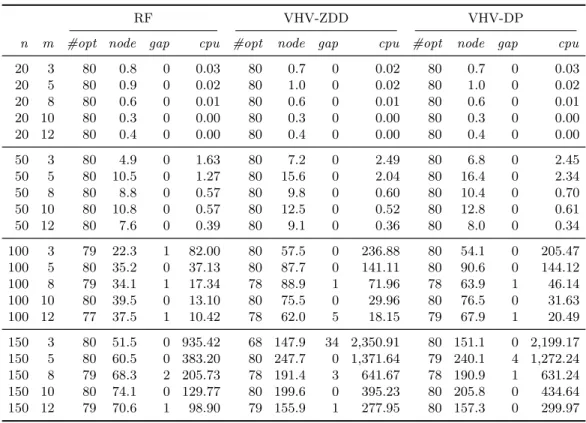
In this section, each run of each algorithm (for one instance) is interrupted after 3600 seconds. The entry gap in the tables is the maximum absolute gap over the unsolved
Table 3 Comparison of the B&P algorithms for instance classes1and2
RF VHV-ZDD VHV-DP
n m #opt node gap cpu #opt node gap cpu #opt node gap cpu 20 3 40 0.9 0 0.03 40 0.8 0 0.02 40 0.9 0 0.02 20 5 40 0.9 0 0.02 40 0.8 0 0.01 40 0.9 0 0.02 20 8 40 0.8 0 0.01 40 0.7 0 0.01 40 0.7 0 0.01 20 10 40 0.5 0 0.01 40 0.5 0 0.01 40 0.5 0 0.00 20 12 40 0.4 0 0.01 40 0.4 0 0.01 40 0.4 0 0.01 50 3 40 3.2 0 1.28 40 2.1 0 0.91 40 1.9 0 0.86 50 5 40 5.2 0 0.74 39 3.3 1 0.55 40 3.7 0 0.60 50 8 40 6.0 0 0.41 39 3.2 1 0.24 39 3.6 1 0.27 50 10 40 5.9 0 0.31 40 2.5 0 0.14 40 2.5 0 0.16 50 12 40 3.2 0 0.12 40 1.8 0 0.08 40 1.7 0 0.10 100 3 40 11.9 0 42.84 40 10.6 0 48.69 40 11.1 0 49.26 100 5 39 25.4 3 44.28 39 31.0 1 70.73 38 21.8 1 46.08 100 8 39 45.7 1 34.66 40 62.8 0 70.28 40 51.3 0 54.06 100 10 39 51.9 1 26.00 40 18.0 0 10.88 40 17.9 0 10.82 100 12 40 68.8 0 29.04 40 86.4 0 38.48 40 89.1 0 38.59 150 3 38 19.4 1 461.09 35 47.6 3 1,058.80 37 40.8 3 935.71 150 5 36 53.9 6 578.85 36 81.3 6 877.32 35 85.6 6 897.39 150 8 35 79.9 13 349.20 36 101.0 6 664.93 36 99.1 9 647.64 150 10 36 117.4 11 354.87 36 78.1 2 322.81 37 97.3 2 411.24 150 12 38 81.9 3 153.79 40 64.8 0 200.96 40 66.8 0 205.59
instances, node is the average number of nodes explored in the B&B tree over the solved instances, and cpu is the average CPU time over the solved instances (in seconds).
Computational results for classes 1 and 2. Table 3 pertains to 40 instances instead of
120. The table shows that the algorithms perform well on the instances of classes 1 and 2. For these two classes, the values of wjpj for everyj∈J are often very different from each other and the final position of every job on its assigned machine is very clear. Consequently, the job-to-machine assignment is crucially important for these instances. For this reason, the number of fractional solutions grows and hence the set covering formulation is less tight, and this is more pronounced for higher n. Algorithms VHV-ZDD and VHV-DP display low running times for instances up to 100 jobs, but the branching has more difficulties to find an optimal solution for higher n. The search requires more nodes and algorithm RF finds optimal solutions more quickly. Overall, all three algorithms solve the problem very well and the average CPU time is low. Algorithm RF performs best especially on instances with 150 jobs with small number of machines. Algorithms VHV-DP and VHV-ZDD are better, however, for instances with 150 jobs when m is higher: they solve more instances and explore fewer nodes in the B&B tree.
Table 4 Comparison of the B&P algorithms for instance classes3−6
RF VHV-ZDD VHV-DP
n m #opt node gap cpu #opt node gap cpu #opt node gap cpu 20 3 80 0.8 0 0.03 80 0.7 0 0.02 80 0.7 0 0.03 20 5 80 0.9 0 0.02 80 1.0 0 0.02 80 1.0 0 0.02 20 8 80 0.6 0 0.01 80 0.6 0 0.01 80 0.6 0 0.01 20 10 80 0.3 0 0.00 80 0.3 0 0.00 80 0.3 0 0.00 20 12 80 0.4 0 0.00 80 0.4 0 0.00 80 0.4 0 0.00 50 3 80 4.9 0 1.63 80 7.2 0 2.49 80 6.8 0 2.45 50 5 80 10.5 0 1.27 80 15.6 0 2.04 80 16.4 0 2.34 50 8 80 8.8 0 0.57 80 9.8 0 0.60 80 10.4 0 0.70 50 10 80 10.8 0 0.57 80 12.5 0 0.52 80 12.8 0 0.61 50 12 80 7.6 0 0.39 80 9.1 0 0.36 80 8.0 0 0.34 100 3 79 22.3 1 82.00 80 57.5 0 236.88 80 54.1 0 205.47 100 5 80 35.2 0 37.13 80 87.7 0 141.11 80 90.6 0 144.12 100 8 79 34.1 1 17.34 78 88.9 1 71.96 78 63.9 1 46.14 100 10 80 39.5 0 13.10 80 75.5 0 29.96 80 76.5 0 31.63 100 12 77 37.5 1 10.42 78 62.0 5 18.15 79 67.9 1 20.49 150 3 80 51.5 0 935.42 68 147.9 34 2,350.91 80 151.1 0 2,199.17 150 5 80 60.5 0 383.20 80 247.7 0 1,371.64 79 240.1 4 1,272.24 150 8 79 68.3 2 205.73 78 191.4 3 641.67 78 190.9 1 631.24 150 10 80 74.1 0 129.77 80 199.6 0 395.23 80 205.8 0 434.64 150 12 79 70.6 1 98.90 79 155.9 1 277.95 80 157.3 0 299.97
Computational results for classes 3−6. Table 4 pertains to the 80 instances of classes
3, 4, 5 and 6. In these classes the processing time pj and weight wj for every j ∈J are
close to each other, and so the ratio between the weight and processing time is close to 1. Consequently, all the jobs have similar priority, and there will be many relevant feasible schedules. The algorithms VHV-DP and VHV-ZDD perform quite weakly on these instances; this was already observed in van den Akker et al. (1999). It is nevertheless surprising that the algorithms require a long time for finding a feasible solution, because the formulation is very tight. This can be explained by the fact that the set covering formulation often returns a fractional solution. The branching strategy of RF clearly needs fewer nodes to find an optimal solution and hence the average runtime over the solved instances is lower. We conjecture that in general, the positions of the jobs in the final solution are more predetermined by assigning two jobs to the same machine or to different machines, rather than by tightening the time window of one job. The position of a job, for these instances, can be easily rearranged without hurting the feasibility and typically entails only a small change of cost. Therefore, branching on the time position only has a limited influence on the set of feasible solutions.
Conclusion. We conclude from Tables 3 and 4 that algorithm RF performs better than algorithms VHV-ZDD and VHV-DP with respect to the number of nodes explored in the B&B tree. The average time per node seems to be equal when one compares the algorithms VHV and RF on the same class of instances, but the clear benefit of the RF branching scheme is that fewer nodes are needed. This has an impact on the total runtime, and leads to better results especially when the number of jobs per machine is high. Consequently, not only stabilization contributes to the efficiency of the algorithm, but also the branching scheme is of vital importance. Only for classes 1 and 2 the algorithm RF performs weakly for instances where the ratio mn is low. One reason for this is that the lower bound of the child nodes is often not much better than the bound of the parent with the Ryan-Foster branching strategy. The branching strategy of van den Akker et al. (1999) performs better when the number of jobs per machine is low. This can be explained by the fact that a tighter time window for a job has a larger influence on the space of feasible solutions if there are not many jobs per machine. Another reason why algorithm RF sometimes fails to find optimal solutions is probably a poor exploration of the B&B tree: we use a hybrid depth-first approach and one of the problems associated with depth-first exploration is trashing, which occurs when different regions of the search fail for the same or a similar reason (see for instance Morrison et al., 2016a). The addition of a single constraint can lead to infeasibility, for example, but this infeasibility might only be detected deeper in the B&B tree.
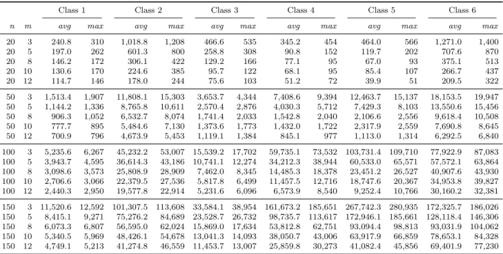
9.4. Evolution of the size of the ZDDs
In Table 5 we report the average (avg) and maximum (max) size of the ZDD (number of nodes) at the root node of the B&B tree for every n, m and instance class. We conclude that the pricing problem is the hardest to solve for the instances with ratio wjpj close to 1 for every jobj. The range of possible processing times and the number of jobs per machine also have a major influence on the size of the ZDDs. For constantn, the size of the ZDDs decreases with increasing m. Overall, the size of the ZDDs is considerable, hence it is important to prevent an additional fast growth upon applying the branching constraints. We also remark that the CPU time for building the ZDD at the root node is very low; on average this is less than 0.06 seconds. This is much lower than the construction times for the maximum independent set problem that are reported in Morrison et al. (2016b).
Table 5 Average and maximum size of the ZDD at the root node
Class 1 Class 2 Class 3 Class 4 Class 5 Class 6
n m avg max avg max avg max avg max avg max avg max 20 3 240.8 310 1,018.8 1,208 466.6 535 345.2 454 464.0 566 1,271.0 1,400 20 5 197.0 262 601.3 800 258.8 308 90.8 152 119.7 202 707.6 870 20 8 146.2 172 306.1 422 129.2 166 77.1 95 67.0 93 375.1 513 20 10 130.6 170 224.6 385 95.7 122 68.1 95 85.4 107 266.7 437 20 12 114.7 146 178.0 244 75.6 103 51.2 72 39.9 51 209.5 322 50 3 1,513.4 1,907 11,808.1 15,303 3,653.7 4,344 7,408.6 9,394 12,463.7 15,137 18,153.5 19,947 50 5 1,144.2 1,336 8,765.8 10,611 2,570.4 2,876 4,030.3 5,712 7,429.3 8,103 13,550.6 15,456 50 8 906.3 1,052 6,532.7 8,074 1,741.4 2,033 1,542.8 2,040 2,106.6 2,556 9,618.4 10,508 50 10 777.7 895 5,484.6 7,130 1,373.6 1,773 1,432.0 1,722 2,317.9 2,559 7,690.8 8,645 50 12 700.9 796 4,673.9 5,453 1,119.1 1,384 845.1 977 1,113.0 1,314 6,292.5 6,840 100 3 5,235.6 6,267 45,232.2 53,007 15,539.2 17,702 59,735.1 73,532 103,731.4 109,710 77,922.9 87,083 100 5 3,943.7 4,595 36,614.3 43,186 10,741.1 12,274 34,212.3 38,944 60,533.0 65,571 57,572.1 63,864 100 8 3,098.6 3,573 25,808.9 28,909 7,462.0 8,345 14,485.3 18,378 23,451.2 26,527 40,907.6 43,930 100 10 2,706.6 3,066 22,379.5 27,536 5,817.8 6,499 11,457.5 12,716 18,747.6 20,367 34,953.8 39,827 100 12 2,440.3 2,950 19,577.8 22,914 5,231.6 6,096 6,573.9 8,540 9,252.4 10,766 30,160.2 32,381 150 3 11,520.6 12,592 101,307.5 113,608 33,584.1 38,954 161,673.2 185,651 267,742.3 280,935 172,325.7 186,026 150 5 8,415.1 9,271 75,276.2 84,689 23,528.7 26,732 98,735.7 113,617 172,946.1 185,661 128,118.4 146,306 150 8 6,073.3 6,807 56,595.0 62,024 15,869.0 17,634 53,812.8 62,751 93,094.4 98,813 93,031.9 104,062 150 10 5,340.5 5,969 48,426.1 54,678 13,041.3 14,093 38,050.7 43,006 63,917.9 66,859 78,653.1 84,328 150 12 4,749.1 5,213 41,274.8 46,559 11,453.7 13,007 25,859.8 30,273 41,082.4 45,856 69,401.9 77,230
Table 6 Evolution of the size of the ZDDs for instances with50jobs
m= 3 m= 5 m= 8 m= 10 m= 12 depth H C H C H C H C H C 5 1.34 −0.04 1.14 −0.02 0.53 0.02 0.20 0.04 0.15 0.07 10 4.20 −0.08 1.83 −0.05 0.93 0.03 0.22 0.07 0.12 0.15 15 7.67 — 1.99 −0.14 1.62 0.08 0.39 0.22 0.51 0.33 20 — — — — 3.17 −0.04 0.76 — — 0.45
Table 6 displays the average growth rate of the size of the ZDDs at various depths of the search tree compared to the size at the root node of the tree, for instances with 50 jobs. For each value of m there are two columns, with H containing the average size using the decision heuristic of Held et al. (2012), and C the average size with the rule introduced in Section 8. A table entry of 1.34, for instance, means that for this setting the average size of the ZDD is around 134% of the size at the root. We report only the values for depths of the B&B tree that are a multiple of 5. For every number of machines we calculate over all six instance classes. We observe that our branching choice allows to control the size of the ZDDs; in some cases the size is even reduced compared to the root node.
10.
Summary and conclusion
In this paper we have augmented the B&P algorithm of van den Akker et al. (1999) by adding several new features such as dual stabilization and Farkas pricing, which are
impor-tant for calculating the LP lower bound at every node of the search tree. Additionally, we have also examined the use of ZDDs for solving the pricing problem. This creates the opportunity to use a generic branching scheme (Ryan and Foster, 1981) for this problem. We have observed that this branching scheme performs very well on instances with which the branching scheme of van den Akker et al. (1999) experienced more difficulties. More generally, this generic branching scheme can be used to solve scheduling problems on paral-lel machines for which the single-machine problem is optimally solved using a priority rule. For future research it would be interesting to evaluate whether it is possible to use ZDDs in the pricing problem for machine scheduling problems that do not have this property.
References
Agarwal, Y., K. Mathur, H.M. Salkin. 1989. A set-partitioning-based exact algorithm for the vehicle routing problem. Networks 19731–749.
Akers, S.B. 1978. Binary decision diagrams. IEEE Transactions on Computers 100509–516.
Azizoglu, M., O. Kirca. 1999. On the minimization of total weighted flow time with identical and uniform parallel machines. European Journal of Operational Research 11391–100.
Belouadah, H., C.N. Potts. 1994. Scheduling identical parallel machines to minimize total weighted comple-tion time. Discrete Applied Mathematics 48201–218.
Ben-Ameur, W., J. Neto. 2007. Acceleration of cutting-plane and column generation algorithms: Applications to network design. Networks 493–17.
Bergman, D., A.A. Cire, W-J. van Hoeve, J.N. Hooker. 2016. Discrete optimization with decision diagrams.
INFORMS Journal on Computing 28 47–66.
Bigras, L-P., M. Gamache, G. Savard. 2008. Time-indexed formulations and the total weighted tardiness problem. INFORMS Journal on Computing 20133–142.
Bruno, J., E.G. Jr Coffman, R. Sethi. 1974. Scheduling independent tasks to reduce mean finishing time.
Communications of the ACM 17382–387.
B¨ulb¨ul, K., H. S¸en. 2017. An exact extended formulation for the unrelated parallel machine total weighted completion time problem. Journal of Scheduling 20 373–389.
Chen, Z-L., W.B. Powell. 1999. Solving parallel machine scheduling problems by column generation.
INFORMS Journal on Computing 11 78–94.
Cire, A.A., W.-J. van Hoeve. 2013. Multivalued decision diagrams for sequencing problems. Operations Research 611411–1428.
Dyer, M.E., L.A. Wolsey. 1990. Formulating the single machine sequencing problem with release dates as a mixed integer program. Discrete Applied Mathematics 26255–270.
Elmaghraby, S.E., S.H. Park. 1974. Scheduling jobs on a number of identical machines. AIIE transactions
61–13.
Fukasawa, R., H. Longo, J. Lysgaard, M.P. de Arag˜ao, M. Reis, E. Uchoa, R.F. Werneck. 2006. Robust branch-and-cut-and-price for the capacitated vehicle routing problem.Mathematical Programming106
491–511.
Held, S., W. Cook, E.C. Sewell. 2012. Maximum-weight stable sets and safe lower bounds for graph coloring.
Mathematical Programming Computation 4363–381.
Hooker, J.N. 2013. Decision diagrams and dynamic programming. International Conference on AI and OR Techniques in Constraint Programming for Combinatorial Optimization Problems. Springer, 94–110. Iwashita, H., S.-I. Minato. 2013. Efficient top-down ZDD construction techniques using recursive
specifica-tions. Tech. Rep. TCS-TR-A-13-69, Hokkaido University, Graduate School of Information Science and Technology.
Knuth, D.E. 2009. The Art of Computer Programming, Volume 4, Fascicle 1: Bitwise Tricks & Techniques; Binary Decision Diagrams. 12th ed. Addison-Wesley Professional.
Lawler, E.L., J.M. Moore. 1969. A functional equation and its application to resource allocation and sequenc-ing problems. Management Science16 77–84.
Lee, C-Y. 1959. Representation of switching circuits by binary-decision programs. Bell System Technical Journal 38985–999.
Lee, C-Y., R. Uzsoy. 1992. A new dynamic programming algorithm for the parallel machines total weighted completion time problem. Operations Research Letters 1173–75.
Lenstra, J.K., A.H.G. Rinnooy Kan, P. Brucker. 1977. Complexity of machine scheduling problems. Annals of Discrete Mathematics 1343–362.
Lopes, M.J.P., J.M.V. de Carvalho. 2007. A branch-and-price algorithm for scheduling parallel machines with sequence dependent setup times. European Journal of Operational Research 1761508–1527. Mehrotra, A., M.A. Trick. 1996. A column generation approach for graph coloring. INFORMS Journal on
Computing 8344–354.
Minato, S.-I. 1993. Zero-suppressed BDDs for set manipulation in combinatorial problems. Proceedings of the 30th International Design Automation Conference. DAC ’93, ACM, New York, NY, USA, 272–277. Morrison, D.R., S.H. Jacobson, J.J. Sauppe, E.C. Sewell. 2016a. Branch-and-bound algorithms: A survey of
recent advances in searching, branching, and pruning. Discrete Optimization 19 79–102.
Morrison, D.R., E.C. Sewell, S.H. Jacobson. 2016b. Solving the pricing problem in a branch-and-price algorithm for graph coloring using zero-suppressed binary decision diagrams. INFORMS Journal on Computing 2867–82.
Pessoa, A., R. Sadykov, E. Uchoa, F. Vanderbeck. 2015. Automation and combination of linear-programming based stabilization techniques in column generation. Tech. Rep. hal-01077984. URL https://hal. inria.fr/hal-01077984.
Pessoa, A., E. Uchoa, M.P. de Arag˜ao, R. Rodrigues. 2010. Exact algorithm over an arc-time-indexed formulation for parallel machine scheduling problems. Mathematical Programming Computation 2
259–290.
Rothkopf, M.H. 1966. Scheduling independent tasks on parallel processors.Management Science12437–447. Ryan, D.M., B.A. Foster. 1981. An integer programming approach to scheduling. A. Wren, ed., Com-puter Scheduling of Public Transport: Urban Passenger Vehicle and Crew Scheduling. North-Holland, Amsterdam, 269–280.
Sadykov, R., F. Vanderbeck. 2013. Column generation for extended formulations. EURO Journal on Com-putational Optimization 181–115.
Smith, W.E. 1956. Various optimizers for single-stage production. Naval Research Logistics Quarterly 3
59–66.
van den Akker, J.M., H. Hoogeveen, S. van de Velde. 2002. Combining column generation and lagrangean relaxation to solve a single-machine common due date problem. INFORMS Journal on Computing 14
37–51.
van den Akker, J.M., J.A. Hoogeveen, S.L. van de Velde. 1999. Parallel machine scheduling by column generation. Operations Research 47862–872.
van den Akker, J.M., C.A.J. Hurkens, M.W.P. Savelsbergh. 2000. Time-indexed formulations for machine scheduling problems: Column generation. INFORMS Journal on Computing 12111–124.
Vance, P.H., C. Barnhart, E.L. Johnson, G.L. Nemhauser. 1994. Solving binary cutting stock problems by column generation and branch-and-bound. Computational Optimization and Applications3111–130. Webster, S. 1992. New bounds for the identical parallel processor weighted flow time problem. Management
Science 38124–136.
Wentges, P. 1997. Weighted Dantzig–Wolfe decomposition for linear mixed-integer programming. Interna-tional Transactions in OperaInterna-tional Research 4151–162.