EXPLORING TRAVEL TIME RELIABILITY USING BLUETOOTH DATA COLLECTION: CASE STUDY IN SAN LUIS OBISPO, CALIFORNIA
A Thesis presented to
the Faculty of California Polytechnic State University, San Luis Obispo
In Partial Fulfillment
of the Requirements for the Degree
Master of Science in Civil and Environmental Engineering
by
Krista Marie Purser June 2016
ii © 2016
Krista Marie Purser
iii
COMMITTEE MEMBERSHIP
TITLE: Exploring Travel Time Reliability using Bluetooth Data Collection: Case Study in San Luis Obispo, California
AUTHOR: Krista Marie Purser
DATE SUBMITTED: June 2016
COMMITTEE CHAIR: Robert Bertini, Ph.D.
Associate Professor of Civil and Environmental Engineering
COMMITTEE MEMBER: Anurag Pande, Ph.D.
Associate Professor of Civil and Environmental Engineering
COMMITTEE MEMBER: Kimberley Mastako, Ph.D.
Lecturer of Civil and Environmental Engineering
iv ABSTRACT
Exploring Travel Time Reliability using Bluetooth Data Collection: Case Study in San Luis Obispo, California
Krista Marie Purser
Bluetooth technology applications have improved travel time data collection efforts and allowed for collection of large data sets at a low cost per data unit. Mean travel times between pairs of points are available, but the primary value of this technique is the availability of the entire distribution of travel times throughout multiple days and time periods, allowing for a greater understanding of travel time variations and reliability. The use of these data for transportation planning, engineering and operations continues to expand. Previous applications of similar data sources have included travel demand and simulation model validation, work zone traffic patterns, transit ridership and reliability, pedestrian movement patterns, and before–after studies of transportation improvements. This thesis investigates the collection and analysis of Bluetooth–enabled travel time data along a multimodal arterial corridor in San Luis Obispo, California. Five BlueMAC devices collected multimodal travel time data in January and February 2016 along Los Osos Valley Road. These datasets were used to identify and process known sources of error such as occasions where vehicles using the roadway turn off and make an
intermediate stop and multiple reads from the same vehicle; quantify travel time performance and reliability along arterial streets; and compare transit, bicycle, and
pedestrian facility performance. Additionally, a travel time model was estimated based on segment characteristics and Bluetooth data to estimate average speeds and travel time distributions.
Keywords: Travel time, travel time reliability, mobility, Bluetooth, travel time modeling, multimodal reliability.
v
ACKNOWLEDGMENTS
Thank you to the BlueMAC manufacturer Digiwest and their parent company Kittelson & Associates, Inc. for their educational discount and technical support. Thank you to the Cal Poly College of Engineering for the funding of the BlueMAC devices. Thank you to the City of San Luis Obispo staff and Cal Poly students who took their time to install the devices, especially Alex Chambers, Bobby Sidhu, Kaylinn Pell, and Bryan Wheeler.
I owe endless thanks to my family and friends who have offered words of
wisdom, encouragement, and patience every step of the way. I would not have succeeded without you. In addition, thank you to the peers who have made each hour spent on campus one of laughter and support. I’m honored to call you a classmate, and more fortunate to call you a friend.
Finally, I am incredibly grateful for the guidance of Drs. Bertini, Pande, and Mastako. Thank you for introducing me to my passion in Fundamentals of Transportation Engineering. Thank you for encouraging me to join the Institute of Transportation
Engineers chapter, for serving as my advisor during internships, and for providing invaluable advice on leadership and vision. Thank you for constantly open office doors, for swift email responses in the late hours of the night, and for giving so much time and energy to your students.
vi
TABLE OF CONTENTS
Page
LIST OF TABLES ... ix
LIST OF FIGURES ... x
LIST OF ACRONYMS ... xii
1. INTRODUCTION ... 1
2. LITERATURE REVIEW ... 2
2.1 Historical Methods of Travel Time Data Collection ... 2
2.1.1 Probe Vehicle ... 2
2.1.2 Remote Sensor & Radar ... 2
2.1.3 License Plate Match ... 3
2.2 Bluetooth Functionality & BlueMAC Devices ... 4
2.2.1 Overview of Bluetooth and MAC Addresses ... 4
2.2.2 Antenna and Range ... 5
2.2.3 Data Capture and Detection Rate ... 6
2.2.4 Known Sources of Error ... 6
2.2.5 Comparison to Other Methods ... 7
2.2.6 Privacy Concerns ... 8
2.3 Transportation Engineering Application of Bluetooth Data Collection ... 8
2.3.1 Multimodal Considerations ... 8
2.3.2 Intelligent Transportation Systems Evaluations ... 9
2.3.3 Model Validation ... 9
2.3.4 Mass Movement Circumstances ... 10
2.3.5 Data Processing Best Practices ... 10
2.3.6 Travel Time Reliability and Performance Metrics ... 11
2.4 Modeling Travel Time ... 13
2.4.1 Mean Travel Time ... 13
2.4.2 Travel Time Variability ... 13
2.5 Summary of Literature Review ... 14
vii
3.1 Study Area ... 15
3.1.1 Study Segments ... 22
3.1.2 Surrounding Land Uses & Future Development ... 26
3.2 Data Collection ... 27
3.2.1 BlueMAC Sensitivity ... 27
3.2.2 BlueMAC Data Collection ... 28
3.2.3 GPS Probes ... 33 3.2.4 Transit Data ... 33 3.3 Configuration Tests ... 34 3.3.1 Automobile ... 34 3.3.2 Bicycle ... 38 4. METHODOLOGY ... 41 4.1 Data Visualization ... 41 4.1.1 Raw Data ... 41 4.1.2 Outlier–Filtered ... 48 4.1.3 Median Method ... 53 5. RESULTS ... 59
5.1 Travel Time Reliability ... 59
5.1.1 Calculation of Reliability Metrics ... 59
5.1.2 Reliability Results ... 60
5.2 Delay Analysis ... 75
5.3 Multimodal Comparison ... 82
5.4 Modeling Average Speed ... 85
5.4.1 Identification of Model Data Inputs ... 86
5.4.2 Model Development ... 86
5.4.3 Findings of Model ... 88
5.5 Modeling Reliability ... 90
5.5.1 Identification of Model Inputs ... 90
5.5.2 Model Development ... 91
5.5.3 Findings of Model ... 93
viii
6.1 Travel Time and Delay ... 96
6.2 Multimodal Comparison ... 96
6.3 Average Speed and Reliability Model ... 97
6.4 Limitations of Research ... 97
6.4.1 Bluetooth Data ... 97
6.4.2 Traffic Counts ... 98
6.4.3 Collision and Incident Comparison ... 99
6.4.4 Modeling Speed and Variability ... 99
6.5 Further Analysis and Research ... 99
ix
LIST OF TABLES
Table Page
Table 1: Detection Rates by Segment, Direction, and Peak Period ... 30
Table 2: Probe Automobile Runs ... 34
Table 3: Probe Bicycle Runs ... 38
Table 4: Raw Data Statistics ... 42
Table 5: Raw Data Error Summary ... 47
Table 6: Outlier–Filtered 1–Variable Statistics ... 48
Table 7: Outlier–Filtered Error Summary ... 52
Table 8: Median Method 1–Variable Statistics ... 53
Table 9: Median Method Error Summary ... 58
Table 10: Higuera to Foothill Data Set Statistics ... 77
Table 11: Transit Reliability on Los Osos Valley Road ... 83
Table 12: Travel Time Reliability Model Inputs ... 86
Table 13: Statistical Significance of Data Model Inputs ... 87
Table 14: Average Speed Model Findings ... 88
Table 15: Gamma Density Function Best–Fit Parameters ... 91
Table 16: K–S Results for Variability Model ... 93
x
LIST OF FIGURES
Figure Page
Figure 1: Bluetooth Sensitivity ... 4
Figure 2: Bluetooth Travel Time Depiction ... 5
Figure 3: Los Osos Valley Road Overview ... 16
Figure 4: Bicycle and Pedestrian Facilities on Los Osos Valley Road ... 17
Figure 5: SLO Transit on Los Osos Valley Road ... 18
Figure 6: Existing and Future Land Uses ... 19
Figure 7: BlueMAC Device Locations ... 20
Figure 8: BlueMAC Device at Madonna Road ... 21
Figure 9: BlueMAC Raw Data Example ... 28
Figure 10: Devices Detected by Number of Intersections ... 29
Figure 11: BlueMAC Detection Rates ... 31
Figure 12: Madonna Road BlueMAC Detection Range ... 32
Figure 13: Geo Tracker Raw Data Example ... 33
Figure 14: Automobile Run #7 Time–Space Diagram ... 35
Figure 15: Automobile Run #9 Time–Space Diagram ... 36
Figure 16: Automobile Run #11 Time–Space Diagram ... 36
Figure 17: Automobile Run #10 Time–Space Diagram ... 37
Figure 18: Automobile Run #12 Time–Space Diagram ... 38
Figure 19: Bicycle Trial Run #1 Time–Space Diagram ... 39
Figure 20: Bicycle Trial Run #2 Time–Space Diagram ... 40
Figure 21: Raw Data Travel Time Example ... 41
Figure 22: Raw Data Travel Time Count Distributions – Northbound ... 42
Figure 23: Raw Data Travel Time Percentage Distributions – Northbound ... 43
Figure 24: Raw Data Travel Time Count Distributions – Southbound ... 43
Figure 25: Raw Data Travel Time Percentage Distributions – Southbound ... 44
Figure 26: Raw Data Time–Space Diagram for Northbound Madonna to Calle Joaquin 45 Figure 27: Raw Data Time–Space Diagram for Southbound Madonna to Calle Joaquin 45 Figure 28: Raw Data Speed Distributions for Northbound Calle Joaquin to Madonna ... 46
Figure 29: Outlier–Filtered Travel Time Count Distributions – Northbound ... 49
Figure 30: Outlier–Filtered Travel Time Percentage Distributions – Northbound ... 49
Figure 31: Outlier–Filtered Travel Time Count Distributions – Southbound ... 50
Figure 32: Outlier–Filtered Travel Time Percentage Distributions – Southbound ... 50
Figure 33: Outlier–Filtered Time–Space Diagram for Northbound Madonna to Calle Joaquin ... 51
Figure 34: Outlier–Filtered Time–Space Diagram for Southbound Madonna to Calle Joaquin ... 52
xi
Figure 36: Median Method Travel Time Percentage Distributions – Northbound ... 54
Figure 37: Median Method Travel Time Count Distributions – Southbound ... 55
Figure 38: Median Method Travel Time Percentage Distributions – Southbound ... 55
Figure 39: Median Method Time–Space Diagram for Northbound Madonna to Calle Joaquin ... 56
Figure 40: Median Method Time–Space Diagram for Southbound Madonna to Calle Joaquin ... 57
Figure 41: Northbound Higuera to Calle Joaquin Travel Time Reliability ... 61
Figure 42: Northbound Higuera to Calle Joaquin Reliability by Time–of–Day ... 62
Figure 43: Northbound Calle Joaquin to Madonna Travel Time Reliability ... 63
Figure 44: Northbound Calle Joaquin to Madonna Reliability by Time–of–Day ... 64
Figure 45: Northbound Madonna to Laguna Travel Time Reliability ... 65
Figure 46: Northbound Madonna to Laguna Reliability by Time–of–Day ... 65
Figure 47: Northbound Laguna to Foothill Travel Time Reliability ... 66
Figure 48: Northbound Laguna to Foothill Reliability by Time–of–Day ... 67
Figure 49: Southbound Calle Joaquin to Higuera Travel Time Reliability ... 68
Figure 50: Southbound Calle Joaquin to Higuera Reliability by Time–of–Day ... 69
Figure 51: Southbound Madonna to Calle Joaquin Travel Time Reliability ... 70
Figure 52: Southbound Madonna to Calle Joaquin Reliability by Time–of–Day ... 70
Figure 53: Southbound Laguna to Madonna Travel Time Reliability ... 71
Figure 54: Southbound Laguna to Madonna Reliability by Time–of–Day ... 72
Figure 55: Southbound Foothill to Laguna Travel Time Reliability ... 73
Figure 56: Southbound Foothill to Laguna Reliability by Time–of–Day ... 73
Figure 57: Coefficient of Variation Comparison ... 74
Figure 58: Level of Service vs. Coefficient of Variation ... 75
Figure 59: Segment Contributions to Northbound Delay by Time–of–Day ... 76
Figure 60: Corridor Northbound Travel Time in the AM Peak ... 78
Figure 61: Corridor Northbound Travel Time in the MID Peak ... 78
Figure 62: Corridor Northbound Travel Time in the PM Peak ... 79
Figure 63: Segment Contributions to Southbound Delay by Time–of–Day ... 80
Figure 64: Corridor Southbound Travel Time in the AM Peak ... 81
Figure 65: Corridor Southbound Travel Time in the MID Peak ... 81
Figure 66: Corridor Southbound Travel Time in the PM Peak ... 82
Figure 67: Northbound Transit and Automobile Standard Deviation ... 83
Figure 68: Southbound Transit and Automobile Standard Deviation ... 84
Figure 69: Northbound Transit and Automobile Coefficient of Variation ... 84
Figure 70: Southbound Transit and Automobile Coefficient of Variation ... 85
Figure 71: Observed vs. Multiple Linear Regression Model Predicted Speeds ... 89
Figure 72: Madonna – Laguna Cumulative Density Plot ... 92
xii
LIST OF ACRONYMS
ADT Average Daily Traffic
dB Decibel
dBi Decibel over Isotropic
dBm Decibel (references to milliwatts)
FAST Act Fixing America’s Surface Transportation Act
FHWA Federal Highway Administration
GPS Global Positioning System
IQR Inter–Quartile Range
ITS Intelligent Transportation Systems
K–S Kolmogorov–Smirnov
MAC Media Access Control
MAP–21 Moving Ahead for Progress in the 21st Century Act
MPH Miles Per Hour
NCHRP National Cooperative Highway Research Program PII Personally Identifiable Information
Q1 First Quartile
Q3 Third Quartile
SHRP2 Second Strategic Highway Research Program STAA Surface Transportation Assistance Act
TMC Transportation Management Center
1
1. INTRODUCTION
As agencies face higher congestion on their built–out roadway networks, methods of increasing capacity shift from additional lanes to increased efficiency of the current physical system. For transportation planners, engineers, and policy–makers, travel time reliability has emerged as both a vital performance measure in maximizing network benefits and an accurate means of identifying locations needing improvement.
Nationwide in 2012, the Moving Ahead for Progress in the 21st Century Act (MAP–21) outlined travel time as a main criterion for allocating funding for transportation projects. More recently in 2015, the Fixing America’s Surface Transportation Act (FAST Act) provides funding and guidance for research and technology programs, such as travel time estimation with emerging technologies. Additionally, the Federal Highway Association allocated funding to the second Strategic Highway Research Program (SHRP2), which sought to establish innovative solutions to improve safety, renewal, capacity, and reliability (FHWA, 2015). The public’s need for travel time estimation and efficient movement extends beyond vehicular user traveler information and daily commutes to multimodal travel decisions and freight movement. The same can be seen internationally as travel time collection methods expand and are further refined.
This thesis aims to evaluate the travel time performance of Los Osos Valley Road as a case study of Bluetooth–collected data, to compare multimodal reliability, to identify effective models for peak period travel times and distributions, and to establish a reliable framework for processing of automated travel time data collection on arterials.
The literature review, research design, methodology, results, and conclusions of this thesis are described in their respective chapters.
2
2. LITERATURE REVIEW
2.1 Historical Methods of Travel Time Data Collection
2.1.1 Probe Vehicle
Often referred to as “floating car” or test vehicle data collection, this method involves sending vehicles into the network for the sole purpose of collecting travel times. The Federal Highway Administration’s (FHWA) Travel Time Data Collection Handbook defines behavior and best practices for Test Vehicle data collection. The personnel within the probe vehicle determine speed of the vehicle based on “average car,” “floating car,” or “maximum car” behaviors. Personnel driving average car attempt to drive the average speed of traffic, floating car attempts to safely pass as many vehicles as it has been passed, and maximum car drives the posted speed limit unless impeded by congestion or safety. Floating car is most common, though in practice the personnel will likely drive a mixture of average car and floating car. Advantages include consistency between data as driving styles are predetermined, complete coverage of the study area, and relatively low initial costs. However, this method leaves room for quality control issues and human error, limits number of network runs and data points, and can be costly to employ personnel (Turner, Eisele, Benz, & Holdener, 1998).
2.1.2 Remote Sensor & Radar
Intelligent transportation systems (ITS) probe vehicle techniques use passive technologies in personal, commercial, and transit vehicles to collect travel times
throughout a network. Data typically reports back to a transportation management center (TMC) in real–time, allowing for ITS applications such as traveler information, real time traffic management, toll collection, bus tracking updates on transit information signs, and
3
route guidance. Advantages include easy and relatively low cost data collection, a continuous data stream, automated collection, data already in electronic format, and no disruption to the typical flow of traffic. Disadvantages can include high initial costs, infrastructure constraints (antenna and coverage issues), requirements of skilled software personnel, privacy concerns, and unnecessary complications when in need of only small scale data collection (Turner et al., 1998).
2.1.3 License Plate Match
License plate matching consists of capturing license plate characters at several points along a network and computing difference in arrival times to yield average speed and travel time along a corridor. Manual license plate match includes personnel recording license plate characters using voice recorders and later transcribing and matching on a computer, typing characters directly onto a computer and later matching, and setting video cameras and later reviewing and transcribing license plates. License plate matching can also be done using video and character recognition software to automatically
transcribe license plates for computer matching. This is often used for freeway/motorway section speed control and enforcement purposes in Europe, and in many U.S. tolling applications for toll payment and/or enforcement. Travel time advantages include potential large samples, continuous travel time data during the study period and short– term analysis, the potential for origin–destination information, and relatively portable data collection equipment. Disadvantages include location limitation in terms of observer safety or video camera positioning, limited study area coverage in one day, highly
4
manual, skilled personnel requirements for data and observation (Turner et al., 1998), and privacy concerns.
2.2 Bluetooth Functionality & BlueMAC Devices
2.2.1 Overview of Bluetooth and MAC Addresses
Bluetooth utilizes radio waves over short–range networks known as piconets to send and receive data. Bluetooth software and products are relatively low cost, utilize less power, and are easy to use. This ease of use led to their use in transmitting data among carry–in and embedded vehicle systems including in–dash navigation and entertainment systems, laptops, phones, tablets, speakers, smartwatches, and headphones (Bluetooth, 2015). An example scenario of detection is shown in Figure 1 (Libelium, 2012).
Figure 1: Bluetooth Sensitivity
BlueMAC is a brand of Bluetooth data collection technology, which utilize Bluetooth to match unique media access control (MAC) addresses between devices,
5
allowing for the calculation of travel time and speed between match points. A diagram depicting the travel time calculation is shown in Figure 2 (Libelium, 2012).
Figure 2: Bluetooth Travel Time Depiction
2.2.2 Antenna and Range
Antenna polarization and gains determine the accuracy and capture rate for Bluetooth data collection on roadways and trails. Antenna polarization includes
directional and omni–directional. Omni–directional antennae send and receive data from any direction while directional only sends and receives data from certain angles in one direction (Abedi, Bhaskar, Chung, & Miska, 2015). Antenna strength is measured in decibels isotropic, or dBi, which correlates to the antenna’s ability to direct or
concentrate radio frequency energy in a particular direction. Omni–directional antennas with gains from 9 to 12 dBi are best for road traffic data collection (Porter, Kim, Magana, Poocharoen, & Arriaga, 2013). While larger antennas provide more gains and more data, they also produce more anomalies and require longer data processing times. Smaller gain
6
antennas have fewer anomalies but produce a smaller sample size. Smaller ranges can be more beneficial to smaller projects with higher pedestrian and cyclist movements (Abedi et al., 2015).
2.2.3 Data Capture and Detection Rate
Data capture and detection rates vary by facility, speed, average daily traffic (ADT), and user type. The location of the Bluetooth device greatly impacts detection rates. A study on detection found a Bluetooth–enabled phone located on an automobile’s dashboard has a three to five times higher detection rate than a Bluetooth–enabled phone in a pocket or purse. In addition, slow–moving vehicles were detected slightly more frequently than fast–moving vehicles due to antenna lag (Stevanovic, Olarte,
Galletebeitia, Galletebeitia, & Kaisar, 2014). A 2.5–mile arterial study with 40,000 ADT on Tualatin–Sherwood Road in Oregon found 3–4% of ADT to be detected (Quayle & Koonce, 2010). With higher amounts of access points, such as driveways and side streets, and longer spacing between devices, it’s likely many of the daily trips do not pass both Bluetooth devices. Additional studies suggest 3–5% (Asudegi, 2009) to 5–10% of ADT can be detected using Bluetooth and MAC matching (Box, 2011).
2.2.4 Known Sources of Error
Sources of error depend on the implementation and facility type associated with the study. Arterials present several challenges to Bluetooth data collection, particularly when compared with freeways. The data collectors should be placed at intersections, where major route decisions become apparent. Appropriate routing between data collectors should be noted, as there are often several possible routes on local networks
7
(Wasson, Sturdevant, & Bullock, 2008). Data processing should account for unusual travel times caused by travel and route choices, such as the following situations:
• A vehicle exits the corridor to access a business, residence, or other destination, then re–enters the corridor later.
• A vehicle chooses a non–direct or unexpected route, where the most direct route is assumed to be taken.
• A vehicle is detected at one device, undetected at the next device, and then potentially detected at a later time or in the opposite direction.
These situations result in apparently increased travel times. In addition,
pedestrian, cyclist, and transit movements along these routes are not distinguished from automobile trips. Vehicles with multiple devices, including carpools and transit, should be processed as well (Quayle & Koonce, 2010). Even with errors, MAC readers can report travel times not significantly different with 95% confidence from Global Positioning System (GPS) devices 83% of the time (Stevanovic et al., 2014).
2.2.5 Comparison to Other Methods
“Ground truth” data can be collected using the more costly test vehicle or
“floating car” data collection methods. While Bluetooth obtains multiple reads from one vehicle, in comparison with GPS which obtains only one read, the Bluetooth reads have been found to be consistent with the ground truth (Koprowski, 2012). In addition, Bluetooth sensors were found to be consistent with ground truth and on par with TRANSMIT data, which utilizes toll collection tags and fixed sensors. Bluetooth was found to outperform INRIX data sets at several study locations (Liu, Chien, & Kim, 2012).
8
2.2.6 Privacy Concerns
Privacy serves as a high concern to the public throughout any traffic data collection procedure. While GPS and cellular phone tracking for the purposes of travel time surveys can contain personally identifiable information (PII), MAC addresses hold no personal information while providing unique codes to match data and provide accurate travel times.
2.3 Transportation Engineering Application of Bluetooth Data Collection
2.3.1 Multimodal Considerations
Bluetooth data collection can assist with improving transit, bicycle, and pedestrian facilities and services. Using Bluetooth to identify commute patterns and origin–
destination data can assess potential ridership of a new transit service. Travel times can improve transit reliability by better estimating travel time, thus attracting more users (Kieu, Bhaskar, & Chung, 2012). In addition, public transportation use can be further studied and estimated to increase ridership and decrease congestion (Weinzerl and Hagemann, 2007). To obtain data on pedestrian and bicycle trips, Bluetooth devices can be placed along multi–use paths or assess the slower moving data on a traditional roadway. Studies should note effects of temperature and weather, purposes of activity (leisure, travel, exercise), and interaction with vehicles and other modes. Pedestrian activity studies should also note buffer zones between building edges and other people as well as road crossing widths and lengths (Abedi et al., 2015). National Cooperative Highway Research Program (NCHRP) Report 797 also notes pedestrians and cyclists tend to make shorter trips, which can be harder to detect (Ryus et al., 2014).
9
2.3.2 Intelligent Transportation Systems Evaluations
Bluetooth travel times can improve pedestrian, bicycle, transit, and automobile activities through ITS. Improved bus travel time data could better facilitate corridor improvements, preparing signals for bus preemption or prioritization. Signal timing could account for heavier incoming vehicles based on their expected travel time, increasing throughput of the system (Kieu et al., 2012). Before and after studies of signal timing changes gauges effectiveness and potential need for further improvement (Quayle & Koonce, 2010). Pedestrian and cyclist activities have provided better information for before and after studies on corridors, allowing for anticipated demand on comparable projects (Ryus et al., 2014).
2.3.3 Model Validation
Bluetooth travel times can validate volume, distance, and origin–destination data to better predict future conditions. Quantifying volumes and modal interaction can better assess risk exposure for different modes (Ryus et al., 2014). In addition, the distance range for pedestrians and cyclists to reach either their destinations or a transit stop can also be verified (Kuzmyak, Walters, Bradley, & Kockleman, 2014). Bluetooth travel times can validate simulations as well (Zhang, Hamedi, & Haghani, 2015). Origin– destination data has been used to gauge network–wide activity and provide appropriate facilities (Wasson et al., 2014). In one particular study, a Bluetooth collection device ran as a floating probe within a commute vehicle for a month on the same route recognized 30% of devices within its range at the end of the month. Commute pattern data gives further information on platooning and transit ridership estimates (Filgueiras et al., 2914).
10
2.3.4 Mass Movement Circumstances
Bluetooth travel times and travel patterns have also been utilized in studying evacuation procedures, work zone effects, and tourism patterns. Evacuation procedures can be improved by recognizing pedestrian bottlenecks and movements, and providing signage or guidance to diffuse or direct crowds. Work zones produce changes to travel patterns, potentially increasing collision risk and endangering construction workers’ safety. Understanding movements in these hazardous conditions can improve safety and efficiency (Abedi et al., 2015). Tourism patterns have also been studied in conjunction with Bluetooth and GPS travel times and patterns. These small–scale studies highlighted popular locations to increase pedestrian facilities and transit service in those areas (Versichele et al., 2014).
2.3.5 Data Processing Best Practices
Due to the presence of multiple transportation modes, driveways and side streets where vehicles can turn off, and multiple devices in one vehicle, data cleaning and processing is necessary to assess data sets before analysis can be conducted. Prior studies have utilized oblique cumulative count curves to assess flow collected by detectors (Bertini, 2006), examined data sets point–by–point to find unrealistic travel times compared to trips made in the same time range (Schneider, Turner, & Wikander, 2010), and removed speeds below the first quartile or above the third quartile in a data set (Li, Chai, & Tang, 2013).
While the point–by–point method can be effective on smaller studies, the level of subjectivity and data processing for this multi–month study would be a dubious and
11
time–intensive method. In addition, the somewhat arbitrary removal of speeds below the first quartile may be ineffective on arterial roadways (Box, 2011).
Maximum error can be determined from the following equation:
E = Zα/2 × 𝑠#
Where n is the minimum sample size, Zα/2 is the standard normal curve area equal to 𝛼/2 for a confidence level of 1–𝛼. s is the standard deviation of the sample, and E is the maximum error of the estimation (Tantiyanugulchai & Bertini, 2003). An error of ±2 mph to ±4 mph may be acceptable (Institute of Transportation Engineers, 2000).
2.3.6 Travel Time Reliability and Performance Metrics
After calculation of the mean travel time and standard deviation of travel time with a reliable data set, further reliability measures can be calculated. Several
straightforward metrics have been proposed, studied and used in various applications. In particular, the Freeway Management and Operations Handbook defines equations for the planning time index, buffer time, buffer index, and coefficient of variation (Neudorff, Randall, Reiss, & Gordon, 2006) which are commonly used reliability measures in the transportation arena. Equations for these values are as follows:
The coefficient of variation is a standardized measure of dispersion of a probability distribution or a frequency distribution:
𝐶𝑜𝑒𝑓𝑓𝑖𝑐𝑖𝑒𝑛𝑡 𝑜𝑓 𝑉𝑎𝑟𝑖𝑎𝑡𝑖𝑜𝑛 = 𝑆𝑡𝑎𝑛𝑑𝑎𝑟𝑑 𝐷𝑒𝑣𝑖𝑎𝑡𝑖𝑜𝑛 𝑜𝑓 𝑇𝑟𝑎𝑣𝑒𝑙 𝑇𝑖𝑚𝑒 (𝑚𝑖𝑛) 𝐴𝑣𝑒𝑟𝑎𝑔𝑒 𝑇𝑟𝑎𝑣𝑒𝑙 𝑇𝑖𝑚𝑒 (𝑚𝑖𝑛)
The buffer index represents the extra time (or time cushion) that travelers must add to their average travel time when planning trips to ensure on–time arrival. For
example, a buffer index of 40 percent means that for a trip that usually takes 20 minutes a traveler should budget an additional 8 minutes to ensure on–time arrival most of the time:
12 𝐵𝑢𝑓𝑓𝑒𝑟 𝐼𝑛𝑑𝑒𝑥
= 95𝑡ℎ 𝑃𝑒𝑟𝑐𝑒𝑛𝑡𝑖𝑙𝑒 𝑇𝑟𝑎𝑣𝑒𝑙 𝑇𝑖𝑚𝑒 𝑚𝑖𝑛 − 𝐴𝑣𝑒𝑟𝑎𝑔𝑒 𝑇𝑟𝑎𝑣𝑒𝑙 𝑇𝑖𝑚𝑒 (𝑚𝑖𝑛) 𝐴𝑣𝑒𝑟𝑎𝑔𝑒 𝑇𝑟𝑎𝑣𝑒𝑙 𝑇𝑖𝑚𝑒 (𝑚𝑖𝑛)
The 8 extra minutes is called the buffer time. Therefore the traveler should allow 28 minutes for the trip in order to ensure on–time arrival 95 percent of the time:
𝐵𝑢𝑓𝑓𝑒𝑟 𝑇𝑖𝑚𝑒 (𝑚𝑖𝑛)
= 95𝑡ℎ 𝑃𝑒𝑟𝑐𝑒𝑛𝑡𝑖𝑙𝑒 𝑇𝑟𝑎𝑣𝑒𝑙 𝑇𝑖𝑚𝑒 𝑚𝑖𝑛 − 𝐴𝑣𝑒𝑟𝑎𝑔𝑒 𝑇𝑟𝑎𝑣𝑒𝑙 𝑇𝑖𝑚𝑒 (𝑚𝑖𝑛)
The planning time index represents how much total time a traveler should allow to ensure on–time arrival. For example, a planning time index of 1.60 means that for a trip that takes 15 minutes in light traffic, a traveler should allow a total of 24 minutes to ensure on–time arrival 95 percent of the time.
𝑃𝑙𝑎𝑛𝑛𝑖𝑛𝑔 𝑇𝑖𝑚𝑒 𝐼𝑛𝑑𝑒𝑥 = 95𝑡ℎ 𝑃𝑒𝑟𝑐𝑒𝑛𝑡𝑖𝑙𝑒 𝑇𝑟𝑎𝑣𝑒𝑙 𝑇𝑖𝑚𝑒 (𝑚𝑖𝑛) 𝐹𝑟𝑒𝑒 𝐹𝑙𝑜𝑤 𝑇𝑟𝑎𝑣𝑒𝑙 𝑇𝑖𝑚𝑒 (𝑚𝑖𝑛)
Prior research has analyzed congestion and percent congested travel as a performance metric (Cambridge Systematics, 2004).Congestion occurs when a
transportation facility experiences higher levels of delay or inconvenience than is deemed acceptable (Meyer, 1998). Delay is defined as the difference between actual travel time and free flow travel time. The amount of delay considered acceptable varies between facility classifications (freeway vs. arterial) and municipalities. In this thesis, the term “congestion” qualitatively describes segments experiencing high traffic densities as well as substantial delays during the designated time period.
13
2.4 Modeling Travel Time
2.4.1 Mean Travel Time
Travel times along a corridor that includes traffic signals can be impacted by intersection and queue delays, with degree of impact related to corridor characteristics. For example, the Highway Capacity Manual (HCM) calculates intersection delay using a ratio of effective green time to cycle length, degree of saturation, and lane group capacity (Transportation Research Board, 2010). Previous studies have identified vehicle–miles traveled (VMT) per lane–mile, driveway density, driveway density per through volume, signal density, signal coordination, and weighted average green time to cycle time for through direction as factors to a travel time estimation model. Light congestion is found to correlate strongly with VMT per lane–mile and weighted average green time, while moderate congestion shows a strong relationship with VMT per lane–mile, driveway density weighted by link through volume, weighted average green time, and signal coordination (Eisele, Zhang, Park, Zhang, & Stensrud, 2011). Stepwise regression is often used to determine statistically significant variables in a model (NCSS, n.d.).
2.4.2 Travel Time Variability
To estimate travel time distributions, portions of the distribution can be attributed to normal, Weibull, and log–normal patterns. Normal distributions reflect travel times under most traffic conditions, Weibull distributions reflect congested traffic, and log– normal distributions reflect free–flow. Previous studies have found variances in what portions can be attributed to each pattern (Li, Chai, & Tang, 2013).
Variability can be estimated with reliability models. Gamma density functions, which skew to the right, are often an adequate fit for travel time distributions on arterials.
14
Gamma density function parameters κ and λ are estimated with regression based on known data. The theoretical κ is then found for each segment using the following equation:
κ = λ ∗ µ
Average travel times, µ, can be estimated with several probe vehicles if not known. Precise travel times are not necessary, as the model was found to not be highly sensitive to travel time estimate error (Polus, 1979). The theoretical and actual κ should be compared via cumulative distribution and a Kolmogorov–Smirnov (K–S) test (NIST Sematech, 2012). If statistically valid via K–S test (O’Connor, 2012), reliability is then estimated with the following equation:
𝑅 = λ µ
This equation is validated to the true reliability, given by the inverse of standard deviation:
𝑅 = 1 𝜎
Prior studies have found R2 for this method to be near 0.37 (Polus, 1979).
2.5 Summary of Literature Review
The low cost per–datum for Bluetooth makes it a viable option for vast and comprehensive data sets. With consideration to known sources of error and Bluetooth functionality, data sets can be processed to provide reliable travel time information, to compare multiple transportation modes, and to build travel time models. This literature review guides the subsequent research design and methodology, and provides insights and explanations to the results and conclusions.
15
3. RESEARCH DESIGN
3.1 Study Area
To better understand the study area and data collection, the following figures and sections summarize existing conditions and future plans for the roadways and
surrounding land uses.
Figure 3 shows the study roadway, where the thickness of Los Osos Valley Road indicates the number of lanes; the thinnest section has one lane in each direction, the medium section has two lanes in each direction, and the thickest section has three lanes in each direction. Intersecting roadways are labeled, signalized intersections are identified, and extents of construction that was underway during data collection are shown. Figure 4 shows bicycle and pedestrian facilities. Figure 5 shows transit routing (City of San Luis Obispo, 2013). Figure 6 shows existing land uses and future development areas.
BlueMAC devices were placed along Los Osos Valley Road at the intersections of Foothill Boulevard, Laguna, Lane, Madonna Road, Calle Joaquin, and South Higuera Street. Figure 7 shows BlueMAC device locations and distances between BlueMAC devices. Devices were placed at these locations due to the heavy amounts of vehicles entering and exiting the corridor at these intersections. Devices were installed on traffic signal poles by City of San Luis Obispo staff. Figure 8 shows the BlueMAC device at Madonna Road.
16
17
18
19
20
21
22
3.1.1 Study Segments
Los Osos Valley Road ranges from two to six lanes in the study area, as indicated by the line thickness in Figure 3. The City of San Luis Obispo classifies Los Osos Valley Road as an arterial from Foothill Boulevard to Madonna Road and Calle Joaquin to South Higuera Street and as a parkway arterial from Madonna Road to Calle Joaquin. Los Osos Valley Road also serves as a designated Surface Transportation Assistance Act (STAA) truck route (City of San Luis Obispo, 2015).
Sidewalks are provided along most of the corridor, with no sidewalks provided from Diablo Drive to Foothill Boulevard, the west side of the roadway from the Froom Ranch Way shopping center to Los Palos Drive, or the east side of the roadway near the 12500 Los Osos Valley Road driveway. Sidewalks were closed near the Los Osos Valley Road and US 101 interchange during construction that was underway from October 2014 through March, 2016. The construction project involved widening Los Osos Valley Road in this section from two to four lanes, with the addition of a new bridge across US 101 and the associated modifications necessary for the freeway ramp terminals. Striped pedestrian crosswalks and pedestrian push buttons are provided along the roadway. The entirety of Los Osos Valley Road provides Class II bicycle facilities, which are standard painted bike lanes adjacent to the traveled lane. A portion of the Bob Jones Trail, a Class I bicycle and pedestrian trail connecting the City of San Luis Obispo to Avila Beach to the south, connects to Los Osos Valley Road near the US 101 Northbound ramps. Bicycle parking and changing locations at public facilities are provided at several points along the roadway. Bicycle lanes were closed near the US 101 interchange during construction, with temporary “Share the Road” signs provided instead (City of San Luis Obispo, 2013).
23
San Luis Obispo Transit Routes 4 and 5 enter and exit the corridor on Foothill Boulevard and Madonna Road, turning around on the Auto Park Way spur, shown in Figure 5. Stops are provided at Los Osos Valley Road at Auto Park Way, Irish Hills, Madonna Road, Laguna Village, Oceanaire, Laguna Lane, Descanso Street, Diablo Drive, and Valley Vista. Both routes run on half–hour headways from 6:30 AM for both routes until 6:30 PM for Route 5 and 10:30 PM for Route 4 on weekdays and 8 AM to 6 PM on weekends and holidays (City of San Luis Obispo, 2013).
The aforementioned Los Osos Valley Road and US 101 interchange construction occurred between the BlueMAC detectors at Higuera Street and Calle Joaquin. One lane was required to be kept open in each direction. Upon completion in March 2016, the interchange provided two lanes in each direction.
Foothill Boulevard is two lanes in the study area. The City of San Luis Obispo classifies Foothill Boulevard as a Regional Route near Los Osos Valley Road. Foothill Boulevard intersects Los Osos Valley Road as a four–legged, signalized intersection with a channelized right–turn lane. Opposite the Foothill Boulevard approach is Sycamore Canyon Road, an unpaved roadway with minimal traffic entering or exiting (City of San Luis Obispo, 2015).
Sidewalks are not provided on this portion of Foothill Boulevard, though striped crosswalks with pedestrian push buttons are available on the south and east side of the intersection. The entirety of Foothill Boulevard provides Class II bicycle facilities. The Los Osos Valley Road bicycle lanes are striped green near the intersection, and the bicycle lane north of the intersection is identified as the Red Davis Bikeway (City of San
24
Luis Obispo, 2013). SLO Transit Routes 4 and 5 enter and exit the Los Osos Valley Road corridor using Foothill Boulevard.
Laguna Lane is a two lane street in the study area. The City of San Luis Obispo classifies Laguna Lane as a local street. Laguna Lane meets Los Osos Valley Road as a signalized t–intersection with two southbound left turn lanes and one southbound right turn lane (City of San Luis Obispo, 2015).
Sidewalks are provided near the intersection, as well as striped crosswalks on the east and north side of the intersection and pedestrian push buttons. A multiuse path is provided along Los Osos Valley Road from Laguna Lane to Oceanaire Drive. No bicycle facilities or transit stops are provided along Laguna Lane (City of San Luis Obispo, 2013).
Madonna Road is classified as a four lane arterial in the study area. Madonna Road meets with Los Osos Valley Road as a four–legged signalized intersection, providing a shared eastbound through and right lane, an eastbound left turn lane, two westbound right turn lanes, one shared westbound through and right lane, and a
westbound left turn lane. Madonna Road also serves as a designated STAA truck route (City of San Luis Obispo, 2015).
Sidewalks are provided near the intersection, as well as pedestrian push buttons and striped crosswalks on all sides. The entirety of Madonna Road provides Class II bicycle facilities. Bicycle parking and changing locations at public facilities are provided at several points along the roadway (City of San Luis Obispo, 2013). SLO Transit Routes 4 and 5 enter and exit the Los Osos Valley Road corridor using Madonna Road.
25
Calle Joaquin is classified as a two lane local road in the study area. Calle Joaquin meets with Los Osos Valley Road as a four–legged signalized intersection, providing one eastbound left turn lane, one eastbound through lane, one channelized eastbound right turn lane, one westbound left turn lane, and one shared westbound through and right lane. Though not designated as an STAA truck route, Calle Joaquin served as a temporary off–ramp during the US 101 interchange construction and carried trucks to the route on Los Osos Valley Road (City of San Luis Obispo, 2015).
Sidewalks are provided near the intersection, as well as pedestrian push buttons and striped crosswalks on all sides. Calle Joaquin provides Class III bicycle facilities (Bike Route, shared use with motor vehicle traffic), though the higher speeds and higher traffic volumes during interchange construction may have shifted bicycle patterns on the roadway (City of San Luis Obispo, 2013). No transit stops are provided along Calle Joaquin.
South Higuera Street is two lanes south and four lanes north of the intersection with Los Osos Valley Road and is classified as an arterial. South Higuera Street meets with Los Osos Valley Road as a signalized t–intersection, with one northbound left turn lane, one northbound through lane, one southbound through lane, and one southbound right turn lane. Higuera Street also serves as a designated STAA truck route (City of San Luis Obispo, 2015).
Sidewalks are provided near the intersection, as well as pedestrian push buttons and striped crosswalks on the west and south side. The entirety of South Higuera Street provides Class II bicycle facilities. Bicycle parking and changing locations at public facilities are provided at several points along the roadway (City of San Luis Obispo,
26
2013). Regional Transit Authority Route 10 runs north and south on South Higuera Street.
3.1.2 Surrounding Land Uses & Future Development
The City of San Luis Obispo Zoning Map shows high amounts of residential and commercial land uses along the Los Osos Valley Road corridor. Housing density ranges from low to high and commercial uses from neighborhood to big–box retail. Several office developments, public parks, and open space are also located along the roadway.
Los Osos Valley Road is poised for future growth. Recent developments include the Prefumo Creek Commons and Irish Hills Plaza, which have increased traffic flows in the area. Completion of the US Highway 101/ Los Osos Valley Road interchange
widening project in March 2016 provides two lanes in each direction and improves ramp intersection operations.
Potential future development and network changes include San Luis Ranch, the Prado Road Interchange, Froom Ranch, and Avila Ranch. San Luis Ranch, Froom Ranch, and Avila Ranch are proposed developments with varying levels of commercial and residential land uses. San Luis Ranch, adjacent to Madonna Road, would potentially occur alongside a future US 101 interchange with Prado Road, and provide alternative routes in the Los Osos Valley Road region of the City. Froom Ranch, proposed to the north of Calle Joaquin and west of Los Osos Valley Road, may increase traffic flows in the area or alter access along Los Osos Valley Road. Avila Ranch, adjacent to South Higuera Street, may increase traffic flows near the southern end of the study area.
27
3.2 Data Collection
3.2.1 BlueMAC Sensitivity
According to the BlueMAC manufacturer, DigiWest, the effective range of the BlueMAC device is estimated by the following calculation:
Responding device Tx power (dBm) + antenna gain (dBi) – free space loss (dB) – fade margin (dB) + BlueMAC antenna gain (dBi) – cable loss (dB) + device Rx sensitivity
(dBm) > 0
Antenna gain and cable loss for the detected devices in this study can be assumed negligible, as virtually all devices have embedded chip antennas and no cables. Thus, the equation becomes:
Responding device Tx power (dBm) – free space loss (dB) – fade margin (dB) + BlueMAC antenna gain (dBi) – cable loss (dB) + device Rx sensitivity (dBm) > 0
The BlueMAC devices have 20 dBm power, equivalent to a Tx Power of 19 dBm. A fade margin is applied to account for physical obstructions or network noise, with 11 dB being industry–standard for reliability (Cameron, 2013). The BlueMAC devices use a standard antenna, which provides a +2.14 dBi gain, and typical cable loss is 1.5 dB (Cameron, 2013). Device sensitivity averages 83 dBm across the study period. Lastly, the free space loss is calculated in terms of distance from the BlueMAC device. The
BlueMAC manufacturer calculates free space loss using the following formula:
Free Space Loss = 20 x Log10 (Frequency in MHz) + 20 x Log10 (Distance in Miles) + 36.6
Bluetooth runs on a 2.4 GHz, or 2400 MHz, frequency. The furthest point in any study intersection from a BlueMAC device is 160 feet. Using 175 feet, or 0.033 miles, to be conservative, the free space loss would be 74.6 dB.
28 The resulting equation is as follows:
19 – 74.6 – 11 + 2.14 – 1.5 + 83 > 0 28.0 > 0
The BlueMAC devices have more than enough signal strength to reliably detect Bluetooth devices at the intersections, creating a clear picture of the corridor.
3.2.2 BlueMAC Data Collection
The BlueMAC devices were stationed along Los Osos Valley Road at
intersections with Foothill Boulevard, Laguna Lane, Madonna Road, Calle Joaquin, and South Higuera Street. Figure 7 shows the detector locations, distances between BlueMAC devices, and mid–study segment signal locations. BlueMAC devices were set to collect continuous data in January and February of 2016, for 60 days’ worth of collection. An example of the data between BlueMAC devices at Madonna Road and Calle Joaquin is shown in Figure 9.
Figure 9: BlueMAC Raw Data Example
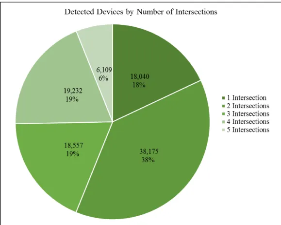
Over 100,000 unique trips were detected. The number of intersections at which Bluetooth devices were detected is shown in Figure 10.
Start Time End Time MAC Travel Time(s) Speed(mph)
1/1/2016 0:09 1/1/2016 0:10 407B81 62 30.3 1/1/2016 0:19 1/1/2016 0:20 B7CF8C 77 24.4 1/1/2016 0:28 1/1/2016 0:30 59906C 109 17.2 1/1/2016 0:44 1/1/2016 0:45 F3E489 87 21.6 1/1/2016 0:48 1/1/2016 0:49 68EAA8 99 19 1/1/2016 0:56 1/1/2016 0:58 BE8A5B 67 28 1/1/2016 1:17 1/1/2016 1:18 6C6175 80 23.5
29
Figure 10: Devices Detected by Number of Intersections
A total of 13 days of data collection, 22% of the study period, had missing segments of data. BlueMAC device at South Higuera Street did not collect data from January 18 at 1:00 AM to January 21 at 9:00 AM due to low battery voltage. BlueMAC device at Calle Joaquin did not collect data from January 19 at 8:00 PM to January 21 at 11:00 AM due to low battery voltage. BlueMAC device at Laguna Lane was unavailable from February 22 at 11:00 AM through the end of February (end of study) for unknown reasons. Despite these small gaps, a robust sample size was available for analysis.
Detection rates for each study segment, direction, and peak period are shown in Table 1 and Figure 11. Data points reflect AM, MID, and PM peak hour volumes versus the average detected devices during that weekday peak hour, averaged over the January 2016 to February 2016 study period and eliminating holidays. Note that these data are for
30
Bluetooth devices detected at two BlueMAC locations versus the City of San Luis Obispo’s 2014 segment counts, and thus ignore vehicles entering or exiting mid– segment. The overall detection rate is 5.7%.
Segment Direction Hourly Detected Devices/Hourly Traffic Count
AM MID PM
Calle Joaquin–Higuera Northbound 26/482 45/822 47/1042
Southbound 47/930 39/786 37/767
Madonna–Calle Joaquin Northbound 32/659 41/1041 52/1353
Southbound 45/839 44/956 39/1022 Laguna–Madonna Northbound 47/721 50/776 74/1218 Southbound 73/1099 54/794 58/876 Foothill–Laguna Northbound 44/615 50/655 67/949 Southbound 59/786 53/646 57/735 Detection 5.7%
31
Figure 11: BlueMAC Detection Rates
Several sources of error for computing travel time would include occasions when vehicles turn off of the roadway into a driveway or side street or the presence of multiple devices in the same vehicle. This includes vehicles that stopped mid–segment at
businesses, residences, or other destinations before continuing along Los Osos Valley Road. Multiple Bluetooth devices may be detected from the same personal or transit vehicle along the route. For example, a driver may have a Bluetooth–enabled smart phone, tablet, laptop, headset and in–dash entertainment or navigation unit. As the corridor serves multimodal trips, several detected trips may be bicyclists or pedestrians. However, the detectors are unable to distinguish between trip modes and thus could not draw conclusive results regarding pedestrian or bicycle travel with Bluetooth data. Along
32
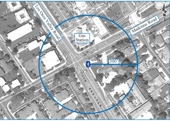
the corridor, several parking lots and gas stations within the detector range and could have skewed travel time data. For example, Figure 12 shows the BlueMAC location and standard 300–foot probable detection radius at the intersection of Madonna Road and Los Osos Valley Road. A vehicle at the gas station on the northern edge of the intersection may be continuously detected as being stopped at the intersection, and thus skew travel time data.
Figure 12: Madonna Road BlueMAC Detection Range
Aside from the ongoing construction at the US 101/ Los Osos Valley Road interchange, no other construction projects were underway along the corridor. Neither incident nor crash data were available for the data collection time frame.
Of the 60 days during January and February 2016 data collection, 15 days had precipitation, with 10 days having more than 0.1 inches of rain. No severe weather conditions were reported during the study period (Weather History for KSBP, 2016).
33
3.2.3 GPS Probes
Twelve probe runs were completed on the corridor during the weekday PM peak period in an automobile and two probe runs were completed during the off–peak period on a bicycle and tracked with the GPS tracking application “Geo Tracker.” Geo Tracker recorded probe runs for comparison to BlueMAC–collected data. An example of the Geo Tracker data is shown in Figure 13.
Figure 13: Geo Tracker Raw Data Example
Automobile probe runs captured the entire corridor, from South Higuera Street to and from Foothill Boulevard. At 95% confidence, the automobile probe runs yielded a maximum error of 3.07 mph, within acceptable range. Bicycle probe runs captured most of the corridor, from Madonna Road to and from Foothill Boulevard. The bicycle probe runs yielded a maximum error of 1.03 mph at 95% confidence, though no acceptable range is established for bicycle data. GPS data were recorded at 1–2 second intervals.
3.2.4 Transit Data
San Luis Obispo Transit uses GPS to track their fleet and stores historical data to evaluate system performance. Historical GPS data of routes 4 and 5, which run along the Los Osos Valley Road corridor, were provided by the Transit app developers, Bishop’s Peak Technology, for the range of February 20, 2016 to March 8, 2016. Collection
type Day Time Latitude Longitude Altitude (m) Speed (km/hr) Distance (km)
T 2/25/2016 12:28:52 AM 35.24 (120.67) 4.00 T 2/25/2016 12:28:54 AM 35.24 (120.67) 4.00 31.40 0.02 T 2/25/2016 12:28:55 AM 35.24 (120.67) 3.00 34.70 0.03 T 2/25/2016 12:28:57 AM 35.24 (120.67) 3.00 35.10 0.05 T 2/25/2016 12:28:59 AM 35.24 (120.67) 3.00 33.80 0.07 T 2/25/2016 12:29:01 AM 35.24 (120.67) 4.00 30.00 0.08 T 2/25/2016 12:29:03 AM 35.24 (120.67) 5.00 22.70 0.10
34
software provides longitude and latitude, vehicle ID, route ID, time stamps, and minutes late from schedule. Transit data were recorded at 15 second intervals.
3.3 Configuration Tests
3.3.1 Automobile
Probe runs in an automobile were conducted along the corridor during the weekday PM peak hour on February 18 and February 24, 2016, with three northbound trips and three southbound trips across the entire corridor each day, for a total of twelve trips. In addition to the Geo Tracker application using GPS to collect travel times along the corridor, a Bluetooth device with a known MAC address in the probe automobile was enabled to compare GPS times to BlueMAC detection times. Table 2 summarizes the probe automobile runs.
Trial
Run Direction Date Time Start
Foothill–Higuera Travel Time (mm:ss) Mean Speed (mph) of Stops Number 1 Southbound 2/18/16 4:20 PM 7:24 25.9 4 2 Northbound 2/18/16 4:30 PM 11:20 16.8 7 3 Southbound 2/18/16 4:44 PM 8:30 22.6 4 4 Northbound 2/18/16 4:54 PM 8:20 23.0 4 5 Southbound 2/18/16 5:04 PM 7:43 24.9 3 6 Northbound 2/18/16 5:14 PM 11:49 16.2 8 7 Southbound 2/24/16 3:35 PM 7:04 27.2 2 8 Northbound 2/24/16 3:44 PM 8:06 23.7 4 9 Southbound 2/24/16 4:01 PM 8:04 23.8 4 10 Northbound 2/24/16 4:11 PM 7:39 25.1 5 11 Southbound 2/24/16 4:21 PM 6:35 29.2 2 12 Northbound 2/24/16 4:30 PM 5:11 37.0 1
Table 2: Probe Automobile Runs
The raw GPS reports were first processed to cut off data beyond the Foothill Boulevard and South Higuera Street intersections, giving the travel times for the study area extents and nothing more. This data can be visualized as trajectories in a time–space
35
diagram, with time on the x–axis, with distance on the y–axis. The GPS data for Trial Run #7 is shown in Figure 14.
Figure 14: Automobile Run #7 Time–Space Diagram
The slope of the line denotes the instantaneous speed (change in distance/change in time) of the automobile. Horizontal lines on the graph show where an automobile was stopped, such as at an intersection or in a queue. To validate BlueMAC accuracy, the automobile probes should be compared to the BlueMAC device data where possible.
For southbound, the personal Bluetooth device was not detected at the Foothill Boulevard nor the Laguna Lane detectors, meaning travel times were not calculated by BlueMAC for either Foothill Boulevard to Laguna Lane or Laguna Lane to Madonna Road. Trials 9 and 11 were only detected at Madonna Road, Calle Joaquin, and South Higuera. Figures 13 and 14 show these trial runs, with the BlueMAC–reported travel time overlaid. As the BlueMAC devices only detect the points of time an automobile passes each location, the automobile’s movements in between devices are not known. Hence,
Foothill Laguna Madonna Calle Joaquin Higuera Descanso Royal Froom Ranch US 101 SB US 101 NB -0.5 1.0 1.5 2.0 2.5 3.0 3.5 00:00 01:00 02:00 03:00 04:00 05:00 06:00 07:00 08:00 09:00 D is ta nc e (m il es ) Time (mm:ss)
36
one can only estimate devices’ average speed across a segment, with no detail as to mid– segment delay. This may be observed in Figures 15 and 16, with no mid–segment details for the BlueMAC data.
Figure 15: Automobile Run #9 Time–Space Diagram
Figure 16: Automobile Run #11 Time–Space Diagram
Foothill Laguna Madonna Calle Joaquin Higuera Descanso Royal Froom Ranch US 101 SB US 101 NB -0.5 1.0 1.5 2.0 2.5 3.0 3.5 00:00 01:00 02:00 03:00 04:00 05:00 06:00 07:00 08:00 09:00 D is ta nc e (m il es ) Time (mm:ss)
Time–Space Diagram, Trial #9, Southbound PM
Probe BlueMAC Foothill Laguna Madonna Calle Joaquin Descanso Royal Froom Ranch US 101 SB US 101 NB -0.5 1.0 1.5 2.0 2.5 3.0 00:00 01:00 02:00 03:00 04:00 05:00 06:00 07:00 08:00 09:00 D is ta nc e (m il es ) Time (mm:ss)
Time–Space Diagram, Trial #11, Southbound PM
Probe BlueMAC
37
For northbound, a similar detection issue occurred. The personal Bluetooth device was only detected at the South Higuera Street and Calle Joaquin detectors during Trial 10 and only detected at the South Higuera Street, Calle Joaquin, and Madonna Road
detectors during Trial 12. Figures 17 and 18 show these trial runs, with BlueMAC– reported detection times and a connecting line overlaid.
Figure 17: Automobile Run #10 Time–Space Diagram
Higuera US 101 SB Froom Ranch Royal Foothill US 101 NB Calle Joaquin Madonna Laguna Descanso -0.5 1.0 1.5 2.0 2.5 3.0 3.5 00:00 01:00 02:00 03:00 04:00 05:00 06:00 07:00 08:00 09:00 D is ta nc e (m il es ) Time (mm:ss)
Time–Space Diagram, Trial #10, Northbound PM
Probe BlueMAC
38
Figure 18: Automobile Run #12 Time–Space Diagram
3.3.2 Bicycle
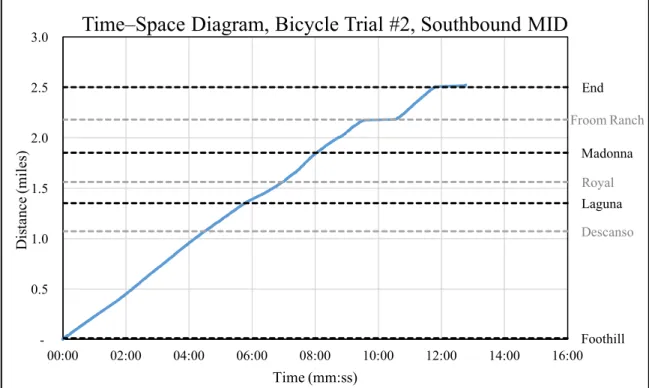
One northbound and one southbound bicycle trip were completed midday on Saturday, February 20 for the majority of the corridor. Due to bike lane closures on the US 101/Los Osos Valley Road interchange during construction, the bicycle trips were conducted from just north of Calle Joaquin to Foothill Boulevard. While a personal Bluetooth device with a known MAC address was enabled, the personal Bluetooth device’s signal was weak and not captured by the BlueMAC devices. Hence, the trial bicycle travel time estimates could not be used to validate BlueMAC–collected bicycle travel times. Table 3 summarizes the probe bicycle runs, and Figures 19 and 20 show the time–space diagrams.
Trial
Run Direction Date Start Time
Foothill–Calle Joaquin Travel Time (mm:ss) Mean Speed (mph) Number of Stops 1 Northbound 2/20/16 11:52 AM 13:43 11.0 1 2 Southbound 2/20/16 12:13 PM 12:46 11.8 1
Table 3: Probe Bicycle Runs
Higuera US 101 SB Froom Ranch Royal Foothill US 101 NB Calle Joaquin Madonna Laguna Descanso -0.5 1.0 1.5 2.0 2.5 3.0 3.5 00:00 01:00 02:00 03:00 04:00 05:00 06:00 07:00 08:00 09:00 D is ta nc e (m il es ) Time (mm:ss)
Time–Space Diagram, Trial #12, Northbound PM
Probe BlueMAC
39
The bicycle runs were completed by a regular cyclist in good health, with minimal additional weight (one lightweight backpack) and a well–operating bicycle. The cyclist did not raise off the bicycle seat and was asked to maintain a non–exerting speed. Other cyclists on the roadway may travel at faster or slower speeds or take breaks.
Figure 19: Bicycle Trial Run #1 Time–Space Diagram
Start Froom Ranch Madonna Royal Laguna Descanso Foothill -0.5 1.0 1.5 2.0 2.5 3.0 00:00 02:00 04:00 06:00 08:00 10:00 12:00 14:00 16:00 D is ta nc e (m il es ) Time (mm:ss)
40
Figure 20: Bicycle Trial Run #2 Time–Space Diagram
Aside from delays toward the southern end of Los Osos Valley Road, bicycle travel speed appears to be constant.
Foothill Descanso Laguna Royal Madonna Froom Ranch End -0.5 1.0 1.5 2.0 2.5 3.0 00:00 02:00 04:00 06:00 08:00 10:00 12:00 14:00 16:00 D is ta nc e (m il es ) Time (mm:ss)
41
4. METHODOLOGY
4.1 Data Visualization
Prior to the determination of delay and travel time estimation, the data must be assessed for validity and processed if the need arises.
4.1.1 Raw Data
Travel time data was collected from January 1, 2016 through February 19, 2016, for a total of 60 days. Figure 21 shows an example of raw travel time data for northbound Calle Joaquin (CP2) to Madonna (CP5).
Figure 21: Raw Data Travel Time Example
42
Segment Direction Length (mi) Travel Time (min) Speed (mph) Speed Limit n
x̄ s x̄ s Higuera–Calle Joaquin NB 0.52 3.3 3.9 15.5 7.8 35 14,540 SB 0.52 2.4 3.0 18.7 7.2 35 14,692 Calle Joaquin– Madonna NB 0.85 8.4 12.3 22.1 15.0 45 24,162 SB 0.85 8.5 12.1 21.1 15.0 45 17,152 Madonna– Laguna NB 0.50 2.2 3.7 24.3 11.5 45 23,412 SB 0.50 2.4 3.8 21.7 10.4 45 19,242 Laguna– Foothill NB 1.35 2.6 4.7 42.9 10.3 45–55 22,584 SB 1.35 3.1 6.3 41.8 11.2 45–55 17,673
Table 4: Raw Data Statistics
Figures 22, 23, 24, and 25 show the travel time distributions by count and percentage frequencies for all study segments for the northbound and southbound directions, respectively. Segment lengths can be found in Table 4. Travel times were binned into 10–second intervals.
Figure 22: Raw Data Travel Time Count Distributions – Northbound
0 500 1,000 1,500 2,000 2,500 3,000 3,500 4,000 4,500 5,000 5,500 6,000 - 2 4 6 8 10 F re que nc y Time (minutes)
Raw Data Travel Time Distributions – Northbound
Calle Joaquin-Higuera Madonna-Calle Joaquin Laguna-Madonna Foothill-Laguna
43
Figure 23: Raw Data Travel Time Percentage Distributions – Northbound
Figure 24: Raw Data Travel Time Count Distributions – Southbound
0% 5% 10% 15% 20% 25% 30% 35% 40% - 2 4 6 8 10 F re que nc y Time (minutes)
Raw Data Travel Time Distributions – Northbound
Calle Joaquin-Higuera Madonna-Calle Joaquin Laguna-Madonna Foothill-Laguna 0 500 1,000 1,500 2,000 2,500 3,000 3,500 4,000 4,500 - 2 4 6 8 10 F re que nc y Time (minutes)
Raw Data Travel Time Distributions – Southbound
Calle Joaquin-Higuera Madonna-Calle Joaquin Laguna-Madonna Foothill-Laguna
44
Figure 25: Raw Data Travel Time Percentage Distributions – Southbound
At first glance, the travel times follow an ‘expected’ distribution. However, consider these segments range from 0.5 miles to 1.35 miles, and a non–trivial amount of trips take more than four minutes. To further evaluate the data, narrowed examinations using time–space diagrams were conducted.
Examining the segment from Madonna Road to Calle Joaquin, which has a 45 mph speed limit and is 0.85 miles long, yields the time–space diagram depicted in Figures 26 and 27 for 4 PM to 5 PM on January 28, 2016 in the northbound and
southbound directions, respectively. Unrealistic data have been identified in red. A free flow trip is shown starting at 4 PM, identified in green. The speed limit along this
segment is 45 mph, with a speed survey showing the 85th percentile speed to be 46 mph. Figure 28 shows raw Bluetooth data’s mean, median, and 85th percentile speeds on a cumulative density plot, as well as the pre–construction 85th percentile speed.
0% 5% 10% 15% 20% 25% 30% 35% 40% - 2 4 6 8 10 F re que nc y Time (minutes)
Raw Data Travel Time Distributions – Southbound
Calle Joaquin-Higuera Madonna-Calle Joaquin Laguna-Madonna Foothill-Laguna
45
Figure 26: Raw Data Time–Space Diagram for Northbound Madonna to Calle Joaquin
Figure 27: Raw Data Time–Space Diagram for Southbound Madonna to Calle Joaquin
0 500 1000 1500 2000 2500 3000 3500 4000 4500 4:00:00 PM 4:30:00 PM 5:00:00 PM D is ta nc e (f ee t) Time
Raw Data Northbound Calle Joaquin to Madonna Time–Space 1/28/16 0 500 1000 1500 2000 2500 3000 3500 4000 4500 4:00:00 PM 4:30:00 PM 5:00:00 PM D is ta nc e (f ee t) Time
Raw Data Southbound Madonna to Calle Joaquin Time–Space 1/28/16
46
Figure 28: Raw Data Speed Distributions for Northbound Calle Joaquin to Madonna
The segment has a maximum northbound travel time of 3050 seconds, or about 51 minutes. Considering several other trips starting at the same time take 2–3 minutes to traverse the segment, this 51–minute trip is more likely to be an occasion where a vehicle turned off the roadway for some purpose and then returned to the roadway than a vehicle traveling at an average speed of 1 mph. Mid–segment land uses include grocery stores, hardware stores, auto dealerships, apartments, fast–food restaurants, big box retail, and many other destinations, increasing the likelihood that vehicles were turning into driveways or side streets.
Longer trips on the roadway are likely to be situations where vehicles turn off of the roadway, pedestrian, or bicycle trips. The data must be further processed to gain an accurate representation of travel times along Los Osos Valley Road. In order to evaluate processing methods, the error should be calculated using the following equation:
47
E = Zα/2 × 𝑠#
The sample size, n, and the standard deviation, σ, will be broken down by AM peak (7 AM – 9 AM), MID peak (11 AM – 1 PM), and PM peak (4 PM – 6 PM) for each segment. Confidence will be set to 95%, resulting in an 𝛼 of 0.05 and Zα/2 of 1.96
(Tantiyanugulchai & Bertini, 2003). The maximum error, E, should be ±4 mph or below (Institute of Transportation Engineers, 2000). To better compare between data processing methods, a “weighted error” is calculated by summing the product of each peak period’s error and sample size, then dividing by the total sample size.
For raw data, the error estimates were as follows:
Segment Direction Error (mph)
AM MID PM
Calle Joaquin–Higuera Northbound 0.46 0.31 0.26
Southbound 0.26 0.31 0.35
Madonna–Calle Joaquin Northbound 0.79 0.69 0.61
Southbound 0.62 0.67 0.76 Laguna–Madonna Northbound 0.50 0.58 0.42 Southbound 0.37 0.44 0.42 Foothill–Laguna Northbound 0.50 0.49 0.40 Southbound 0.43 0.52 0.49 Weighted Error 0.48 mph
Table 5: Raw Data Error Summary
These results are reasonable given the large sample size, resulting in a weighted error of 0.48 mph. However, Figures 24 and 25 highlight that some data points are unreasonable and should be removed from the analysis dataset. Several data filtering methodologies were identified in the literature review; filtering methodologies in this thesis are the Outlier–Filtered and Median Method, further described in the following sections.