Short term wind speed prediction using Multi Layer Perceptron
M. Beccali1 , S. Culotta*2, V. Lo Brano 3
Dipartimento dell’Energia, Università degli Studi di Palermo. Italy e mail: [email protected];
e mail: [email protected] e mail: [email protected]
ABSTRACT
Among renewable energy sources wind energy is having an increasing influence on the supply of energy power. However wind energy is not a stationary power, depending on the fluctuations of the wind, so that is necessary to cope with these fluctuations that may cause problems the electricity grid stability. The ability to predict short-term wind speed and consequent production patterns becomes critical for the all the operators of wind energy. This paper studies several configurations of Artificial Neural Networks (ANN), a well-known tool able to estimate wind speed starting from measured data. The presented ANNs, t have been tested through data gathered in the area of Trapani (Sicily). Different models have been studied in order to determine the best architecture, minimizing statistical error. Simulation results show that the estimated values of wind speed are in good accord with the values measured by the anemometers.
Keywords: Artificial neural networks, Multi layer perceptron, Feed forward network Forecasting, Renewable energy, Wind energy, Wind speed
INTRODUCTION
Among the renewable resources the one that had a faster technological innovation and a more rapid diffusion is wind energy. The power generated by wind turbines depends on the intensity and persistence of the wind in the area under consideration. Therefore a good knowledge of the characteristics of the wind is a prerequisite for a good planning and construction of any wind power project. In the literature several statistical methods are reported to estimate the wind speed [1,2,3]. These methods aim to find the relationships between the climatic data recorded in the site and then the quality of the collected data is extremely important.
The simple knowledge of wind speed data is not sufficient to calculate the energy production available in a site. To get more complete information is necessary to know probability distribution of wind speed over the time.
In fact the knowledge of the probability density functions (PDF) of the wind speed is very important for the assessment of the performance of wind turbines. Actually, the quality of the productivity analysis in wind farm planning depends on the capability of the PDF, for example the Weibull distribution, to describe the measured wind speed frequencies distribution [4,5].
Anyway, because the wind is an intermittent resource the instantaneous power generated by a wind farm varies rapidly. The fluctuation of wind power generation in many cases causes problem of grid stability [6, 7]. For this reason becomes crucial to apply forecasting methods of the wind speed and the consequent production of a wind energy installation in the short term, i.e. some hours.
The learning approach, based on artificial neural networks, is a valid tool to predict wind speeds. ANNs have the capability to process complex input-output data sets (even if not physically related) in order to forecast an event starting from learning of a past phenomenon.
Artificial neural networks are network systems which are built by simulating the learning behavior of human being [8]. In fact they have the ability to learn from past experience and then apply their knowledge to new event. There are many different typologies of ANN [9] but in this study the Multi Layer Perceptron (MLP), also called feed forward network, has been used for predicting the wind speed [10].
In this work different configurations of MLP have been proposed in order to find the best exploitation of the wind data in gathered in the area of Trapani (Sicily). Three different models with single or double hidden layers (and with a different number of neurons) have been tested in order to find the best network architecture [11].
ARTIFICIAL NEURAL NETWORKS
In the last years the artificial neural networks have been applied in different sectors like engineering, medicine, physics. In fact they can be used in problems of prediction, classification or control. ANNs are indeed a tool for modelling and forecasting, which is widely used as a valid alternative to solve complex problems arising when variables are not clearly related by physical laws.
The ability of the ANN to approximate large classes of non-linear functions with a good accuracy makes them very appropriate for the representation of dynamic non-linear systems [12]. Artificial neural networks are characterized by an interconnection of few simple elements whose functionality is based on the human biological neurons.
There are several typologies of neural networks described in literature (Feedforward neural network, Kohonen self-organizing network, Radial basis functions, Recurrent neural network etc..) but in this study the Multi Layer Perceptron (MLP), also called feed forward network, has been used for predicting the wind speed.
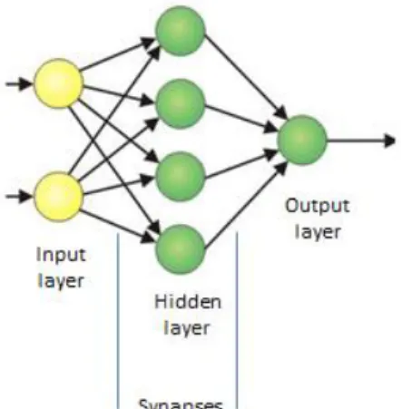
The communication within the network is based on a layered structure. Each layer makes independent computations. The first and the last layers are respectively the input and output layers. The layers placed between those are the hidden layers [13]. The neurons (or processing elements) of the hidden layer receive information from the previous layer and are related with neuron of the next layer. They can only interact with neurons of the neighbouring layers while there are no connections between the neurons of the same level. Each processing element makes its computation based upon a weighted sum of its inputs.
Figure 1 show a generic topology of artificial neural network.
The basic elements in the neuron model are the synapses and the activation function (back propagation algorithm). The synapses are represented as connections between units.
Input initializes the activation weightings of the neurons in the input layers.
The activation level on the first layer is the then passed to the next layer. The set of the weights to be applied to these inputs is re-calculated in every calculation step by a back propagation algorithm in order to minimize the squares of the differences between the actual and the desired outputs.
Figure 1. The neural network architecture
Different configurations of MLP based on variable number of layers and neurons have been studied for the specific application to Trapani (Sicily).
Three different models with single or double hidden layers (and with a different number of neurons) have been verified in order to identify the best neural architecture able to provide a short–term wind speed forecasting. In a first step of this study data collected by two anemometers with the frequency ten minutes have been utilised. In a second phase data captured every ten minutes have been averaged in order to obtain hourly figures.
DESIGN PROCESS OF ANN SYSYSTEM
The process of set-up and validation of a neural system [14] generally includes the following steps:
• Data acquisition and pre-processing; • Statistical analysis and normalization; • Design of ANN structure;
• Training and validation phases; • Testing phase.
Usually the design process is iterative. In fact it is possible that a particular structure falls on default in one of the steps listed above. In this situation it is necessary to change the model and the ANN should be retrained [15].
The wind speed data vectors, v1 and v2, adopted in this study, have been acquired by two anemometers installed at hub height of 50 m with a frequency of ten minutes [7]. The data set contains the wind speed recorded from 28 April 2005 to March 2008.
As a preliminary phase, it was necessary to process the raw data in order to assess their quality. To fulfil this task it is necessary to identify, according to the period of observation, the expected number of data, the number of missing data, the number of data with not null wind speed, the measurements of calm and discard incorrect values.
In order to have further confirmations of the consistence and reliability of the data it is possible to perform additional statistical analyses such as the calculation of Weibull or Rayleigh distributions.
Once the pre-processing phase has been fulfilled, data are normalized and processed through a correlation analysis in order to identify the best period of data set to be used in the training and in the testing phases [14]. The aim of this analysis is to assess the strength of a linear or nonlinear relationship between the two vectors v1 and v2. The correlation coefficient can assume values
between -1 and 1. It is equal to -1 when there is a negative correlation between the two data sets, is equal to 0 when data are not correlated and to 1 when there is a positive correlation.
During the training phase the best data set is represented by the one with the best correlation coefficient while during the testing phase the data with the worst correlation must be used. From the result of correlation analysis (Table 1) authors decided to use the data measured in May 2006 for the training phase and the data detected in May 2005 for the testing phase.
Table 1. Result of correlations Month Correlation coefficient
2005 2006 2007 January 1 1 February 0.99 1 March 1 1 April 0.87 1 0.99 May 0.80 1 1 June 0.86 1 1 July 0.85 1 1 August 0.81 1 1 September 0.85 1 1 October 0.88 1 1 November 0.82 1 1 December 0.84 1 1
In order to control the generalization ability of the network in adapting the experience acquired in the training phase, the technique of cross validation (CV) has been applied. With the cross validation the data of training phase are divided in a subset of estimation and a subset of validation. The first subset (70 % of data) is used to obtain estimates of parameters and the second (30% of data) is used to validate the performance of the estimate.
In order to identify the best model among the ones analysed, authors have adopted the criteria of minimization of the Mean Square Error (MSE) with a tolerance limit set to 20% [16].
If yt is the actual observation for a time period t and Ft is the forecast for the same period, the error is the MSE can be defined by:
2 1 1 ; n t t t t t MSE e e y F n (1)
Where n is the number of periods of steps.
The MSE was calculated not only during the training phase but also in the validation and testing phases.
PROPOSED MODELS OF MULTY LAYER PERCEPTRONS FOR PREDICTION OF WIND SPEED
Three different configurations of MLP with different complexity have been tested to perform forecast of wind speed data from one to five time steps forward.
The network called “Low” has only one hidden layer, the “Medium” and “High” networks have two hidden layers but a different number of neurons. The input data that were provided to the
networks are the wind speeds v1 and v2 recorded by two anemometers placed in the same area. The forecast processing was carried out for different number of time steps (ten minutes): from zero to five.
Above the described configurations the authors have tested the following networks: - Networks v1-v1 where v1 is used as input and output;
- Networks v2-v2 where v2 is used as input and output;
- Networks v1v2-v1 where v1 and v2 are the input data and the output is the speed v1; - Networks v1v2-v2 where v1 and v2 are the input data and the output is the speed v2.
Therefore the acronym of the different models is composed by three elements: input data vector, forecast length and type of architecture. For example in the network (v1_1_L), in table 2, v1 is the input, 1 is the forecast horizon (ten minutes) and L is the network architecture with low complexity.
The obtained results are presented in following tables. Tables 2 and 3 show the calculated MSE for the networks with only one input while tables 4 and 5 show the MSE for the networks with two inputs.
It is worth noting that the ANNs with two inputs and one hidden layer (Low) are certainly the best models.
Table 2. Mean square errors for the neural networks with v1 for input and output
Network MSE Train MSE CV MSE Test
v1_0_L 0.00000057 0.00000076 0.0000000001 v1_1_L 0.00334762 0.00364580 0.0000000067 v1_2_L 0.00612936 0.00733753 0.0000000280 v1_3_L 0.00886840 0.01067830 0.0000000644 v1_4_L 0.01090821 0.01365200 0.0000000781 v1_5_L 0.01344239 0.01625730 0.0000001005 v1_0_M 0.00067529 0.00106042 0.0000001165 v1_1_M 0.00679159 0.00922480 0.0000005620 v1_2_M 0.00670291 0.00871230 0.0000001430 v1_3_M 0.01405680 0.01887690 0.0000009275 v1_4_M 0.01154532 0.01509001 0.0000002109 v1_5_M 0.01433278 0.01888038 0.0000004094 v1_0_H 0.00796097 0.01493450 0.0000016659 v1_1_H 0.00815784 0.01453130 0.0000010978 v1_2_H 0.00960655 0.01253950 0.0000008668 v1_3_H 0.01189107 0.01417621 0.0000007623 v1_4_H 0.01303969 0.01830570 0.0000005747 v1_5_H 0.01364650 0.01839424 0.0000003863
Table 3. Mean square errors for the neural networks with v2 for input and output
Network MSE Train MSE CV MSE Test
v2_0_L 0.00000050 0.00000074 0.00001712 v2_1_L 0.00340190 0.00362519 0.00013141 v2_2_L 0.00621156 0.00734003 0.00087517 v2_3_L 0.00898109 0.01069069 0.00082469 v2_4_L 0.01131379 0.01359214 0.00140055 v2_5_L 0.01305820 0.01604964 0.00197225 v2_0_M 0.00055900 0.00082680 0.33980218
v2_1_M 0.00863774 0.01140980 0.01276821 v2_2_M 0.00662890 0.00841130 0.00180536 v2_3_M 0.00930510 0.01175050 0.00264751 v2_4_M 0.01421550 0.01824130 0.00948332 v2_5_M 0.01338553 0.01659220 0.00320692 v2_0_H 0.01809274 0.01411125 0.00685920 v2_1_H 0.00651950 0.01033940 0.01272843 v2_2_H 0.00956068 0.01018382 0.00780280 v2_3_H 0.01228585 0.01855370 0.01446880 v2_4_H 0.01329478 0.01839603 0.00463121 v2_5_H 0.01741058 0.02189950 0.01481504
Table 4. Mean square errors for the neural networks with two input and v1 for output
Network MSE Train MSE CV MSE Test
v1v2_0_L 0.000000224 0.000000273 0.000000000028 v1v2_1_L 0.003223600 0.003619700 0.000000013944 v1v2_2_L 0.006275820 0.007637000 0.000000047509 v1v2_3_L 0.008872400 0.010854700 0.000000099515 v1v2_4_L 0.011205780 0.013751800 0.000000108993 v1v2_5_L 0.013488754 0.016417000 0.000000132973 v1v2_0_M 0.000566651 0.000918420 0.000000092089 v1v2_1_M 0.003652880 0.004586410 0.000000093628 v1v2_2_M 0.006553250 0.008482700 0.000000114684 v1v2_3_M 0.008933580 0.011280140 0.000000113543 v1v2_4_M 0.011352500 0.014577740 0.000000164365 v1v2_5_M 0.013218870 0.016708900 0.000000181975 v1v2_0_H 0.003021920 0.006362070 0.000000639601 v1v2_1_H 0.006717400 0.012650300 0.000000957869 v1v2_2_H 0.011288290 0.018646500 0.000001318420 v1v2_3_H 0.022805550 0.030301200 0.000000460971 v1v2_4_H 0.013574470 0.022353800 0.000001217575 v1v2_5_H 0.015183530 0.021027510 0.000001066649
Table 5. Mean square errors for the neural networks with two input and v2 for output
Network MSE Train MSE CV MSE Test
v1v2_0_L 0.00008500 0.00023692 0.0000000203 v1v2_1_L 0.00322066 0.00367138 0.0000236788 v1v2_2_L 0.00617680 0.00753680 0.0000000965 v1v2_3_L 0.00881186 0. 0107297 0.0000231019 v1v2_4_L 0.01110347 0.01348470 0.0000001620 v1v2_5_L 0.01288910 0.01609230 0.0000001725 v1v2_0_M 0.00063298 0.00091802 0.0000001037
v1v2_1_M 0.00381116 0.00488440 0.0000001205 v1v2_2_M 0.00977035 0.01310015 0.0000005951 v1v2_3_M 0.00910830 0.01173160 0.0000001512 v1v2_4_M 0.01134850 0.01458897 0.0000001782 v1v2_5_M 0.01327440 0.01690310 0.0000001974 v1v2_0_H 0.00785680 0.00788916 0.0000238310 v1v2_1_H 0.00553737 0.00772170 0.0000005244 v1v2_2_H 0.00810041 0.01104280 0.0000005570 v1v2_3_H 0.01281810 0.01865220 0.0000008167 v1v2_4_H 0.01555260 0.02733420 0.0000018408 v1v2_5_H 0.01591726 0.02334670 0.0000012571
A further comparison of the network architectures with the lowest values of MSE has been done by assessing the average and standard deviation of desired and actual outputs and thus percent deviation between the generated and that expected values. The results of the Table 6 show that the smaller values of percent deviation are obtained for networks with two inputs and v1 as outputs.
Table 6. Analysis of MSE
Networks Desired output Actual output Percent Deviation
v1_0_L – v1 Average 5.68 5.68 0.03 St. Deviation 3.76 3.76 0.03 v1_0_M- v1 Average 5.68 5.77 1.54 St. Deviation 3.76 3.79 0.72 v1_1_H- v1 Average 5.68 5.71 0.44 St. Deviation 3.76 3.77 0.21 v2_0_L-v2 Average 5.68 5.73 0.12 St. Deviation 3.76 3.72 0.36 v2_2_M-v2 Average 5.68 5.77 0.82 St. Deviation 3.76 3.60 3.12 v2_4_H-v2 Average 5.68 5.72 0.10 St. Deviation 3.76 3.30 11.13 v1v2_0_L-v1 Average 5.72 5.73 0.15 St. Deviation 3.71 3.74 0.71 v1v2_0_M-v1 Average 5.72 5.80 1.42 St. Deviation 3.71 3.75 1.16 v1v2_0_H-v1 Average 5.72 4.71 17.70 St. Deviation 3.71 3.91 5.26 v1v2_0_L-v2 Average 5.68 5.68 0.002 St. Deviation 3.76 3.76 0.018 v1v2_0_M-v2 Average 5.68 5.77 1.572 St. Deviation 3.76 3.78 0.601 v1v2_0_H-v2 Average 5.68 5.50 3.215 St. Deviation 3.76 3.49 7.215
Authors have carried out an additional analysis in which the data collected every 10 minutes were averaged on hourly basis. The same structures of ANN have been used for the wind speed hourly prediction. In this case the network output is a vector of five hourly values. The results obtained show that the best networks are those having low complexity and v1 as output. Compared to the networks application for the forecast of values for sampled every 10 minutes, there is an increase of the error. Table 7 and 8 show respectively the values of MSE for the networks with hourly forecast with one or two inputs and v1 for output. Table 9 shows the average, the standard deviation and the percent deviation between the value generated and the one expected.
Table 7. Mean square errors for forecasting max five values of hourly averaged data with v1 for input and output
Network MSE Train MSE CV MSE Test
v1_0_L 0.000001 0.000001 0.000000000024 v1_1_L 0.009653 0.012356 0.000000008450 v1_2_L 0.019907 0.026790 0.000000024770 v1_3_L 0.028060 0.037530 0.000000109036 v1_4_L 0.035672 0.043502 0.000000098429 v1_5_L 0.0134423 0.0162573 0.000000184865 v1_0_M 0.000301 0.000409 0.000000007951 v1_1_M 0.009632 0.014203 0.000000025767 v1_2_M 0.019786 0.029321 0.000000072453 v1_3_M 0.025815 0.042474 0.000000155792 v1_4_M 0.034670 0.044968 0.000000191115 v1_5_M 0.039508 0.053926 0.000000260284 v1_0_H 0.000335 0.000400 0.000000010828 v1_1_H 0.010180 0.013291 0.000000027174 v1_2_H 0.020149 0.028046 0.000000076288 v1_3_H 0.029159 0.039595 0.000000208403 v1_4_H 0.037417 0.045626 0.000000274167 v1_5_H 0.042210 0.049784 0.000000207080
Table 8. Mean square errors for forecasting max five values of hourly averaged data with two input and v1 for output
Network MSE Train MSE CV MSE Test
v1v2_0_L 0.000173 0.000030 0.0000000003 v1v2_1_L 0.009646 0.012127 0.0000000100 v1v2_2_L 0.010572 0.027039 0.0000000269 v1v2_3_L 0.027485 0.039845 0.0000001309 v1v2_4_L 0.034067 0.048339 0.0000000892 v1v2_5_L 0.039193 0.056843 0.0000001295 v1v2_0_M 0.002246 0.000342 0.0000000058 v1v2_1_M 0.009305 0.013672 0.0000000247 v1v2_2_M 0.018654 0.030343 0.0000000943 v1v2_3_M 0.024841 0.046203 0.0000001668 v1v2_4_M 0.031165 0.065871 0.0000002135 v1v2_5_M 0.034898 0.062296 0.0000002843
v1v2_0_H 0.000476 0.000770 0.0000000148 v1v2_1_H 0.010233 0.013212 0.0000000335 v1v2_2_H 0.019692 0.027589 0.0000000802 v1v2_3_H 0.027757 0.038128 0.0000001718 v1v2_4_H 0.033721 0.052073 0.0000003490 v1v2_5_H 0.051663 0.053404 0.0000007377
Table 9. Analysis of MSE for the best neural networks architectures for hourly forecast
Networks Desired output Actual output Percent Deviation
v1_0_L Average 5.69 5.69 0.02 St. Deviation 3.66 3.67 0.04 v1_0_M Average 5.69 5.73 0.72 St. Deviation 3.66 3.71 1.14 v1_1_H Average 5.69 5.74 0.96 St. Deviation 3.66 3.66 0.11 v1v2_0_L Average 5.69 5.69 0.06 St. Deviation 3.66 3.67 0.08 v1v2_0_M Average 5.69 5.73 0.70 St. Deviation 3.66 3.69 0.82 v1v2_0_H Average 5.69 5.77 1.44 St. Deviation 3.66 3.67 0.06
Table 9 shows that the network with architecture Low have the lower values of percent deviation compared to more complex architectures. Comparing the results with the same networks with a time step of ten minutes we have a decrease in the performance while remaining within the limit of 20%.
CONCLUSION
Speed profiles of the wind are known for having a great variability in time due to a stochastic nature of the driving phenomena. Mapping and modelling of wind speed are the essential prerequisite for any wind energy project. Therefore, the conversion and efficient utilization of wind energy resource needs an accurate knowledge of the wind characteristics on the site under investigation.
Artificial neural networks can be a valuable tool for short term prediction. Indeed they are characterized by an adaptive nature in which “learning through example” replaces classical physical or statistical models. This characteristic makes the ANN techniques very attractive to solve non-linear phenomena.
In this study different configurations of neural networks have been generated and tested to predict the wind speed. In order to compare the performances of several architectures and then to assess the best model the statistical standard error has been considered.
The result obtained are in good agreement with the measured values for many ANN configurations.
The simplest models have better performance than the more complex ones either in training either in testing phases, well describing the presence of the wind in the area where the data was collected.
By increasing the complexity of the network and the number of the input the MSE assumes highest values, however, remaining under the tolerances limit set to 20%.
REFERENCES
1. Vogiatzis N., Kotti K., Spanomitsios S., Stoukides M., Analysis of wind potential and characteristics in North Aegean, Greece. Renewable Energy, 29, pp 1193–1208, 2004. 2. Ucara A., Balo F., Investigation of wind characteristics and assessment of
wind-generation potentiality in Uludag˘- Bursa, Turkey. Applied Energy, 86, pp 333–339, 2009.
3. Cancino-Solorzano Y., Xiberta-Bernat J., Statistical analysis of wind power in the region of Veracruz (Mexico). Renewable Energy, 34, pp1628–1634, 2009.
4. Lo Brano V., Orioli A., Ciulla G., Culotta S., Quality of wind speed fitting distributions for the urban area of Palermo, Italy. Renewable Energy, 36 pp. 1026 – 1039, ISSN: 0960-1481, 2011.
5. Ali Naci Celik. On the distributional parameters used in assessment of the suitability of wind speed probability density functions. Energy Conversion and Management, 45, pp 1735–1747, 2004.
6. Gong Li, Jing Shi, Junyi Zhou., Bayesian adaptive combination of short- term wind speed forecast from neural networks models. Renewable Energy, 36, pp 352–359, 2011.
7. Beccali M., Culotta S., Galetto J. M.,. Macaione A,. Influence of raw data analysis for the use of neural networks for wind farms productivity prediction. International Conference
on Clean Electrical Power - ICCEP 2011. Ischia (italy), 14-16 June 2011, pp.791-796.
VDE VERLAG Conference Proceedings
8. Sağbaş A., Karamanlıoğlu T., The Application of Artificial Neural Networks in the estimation of Wind Speed: A case study. 6th International Advanced Technologies
Symposium (IATS’11), 16-18 May 2011, Elazığ, Turkey
9 Rojas R. Neural Networks: A Systematic Introduction. Springer – Vergar, Berlin 1996 10. Sreedevi M., P. Jeno Paul. New Intelligent Technique for Estimating the Parameters of
Wind Energy Conversion System. International Journal of Soft Computing 6 (1) pp 6-10, 2011.
11. Fadare D.A., The application of artificial neural networks to mapping of wind speed profile for energy application in Nigeria. Applied Energy, 87, pp.934–942, 2010.
12. Cellura M., Culotta S., Lo Brano V., Marvuglia A., (2011), Nonlinear black-box models for short-term forecasting of air temperature in the town of Palermo. In: Geocomputation,
Sustainable and Environmental Planning, Series: Studies in Computational Intelligence, Murgante, Beniamino; Borruso, Giuseppe; Lapucci, Alessandra (Eds). 1st Edition., 2011, 279 p., Hardcover ISBN: 978-3-642-19732-1. Springer-Verlag, Berlin/Heidelberg;
13. Campbell P.R.J. and Adamson K., A Novel Approach to wind forecasting in the United Kingdom and Ireland I.J. of SIMULATION V. 6 No 12-13 ISSN 804x online, 1473-8031 print.
14. Sreelakshmi K., Ramakanthkumar P., Neural Networks for Short Term Wind Speed Prediction. World Academy of Science, Engineering and Technology, 42 2008.
15. Yurdusev M. A., Ata R., Cetin N.C., Assessment of optimum tip speed ratio in wind turbines using artificial neural networks. Energy, 31, pp1817-1825, 2006
16. El-Shafie A., Noureldin A.E., Taha M.R., Basri H., Neural Network Model for Nile River Inflow Forecasting Based on Correlation Analysis of Historical Inflow Data. Journal of