2-25-2018
Work‐Efficient Parallel Union‐Find
Natcha Simsiri
University of Massachusetts Amherst
Kanat Tangwongsan
Mahidol University International College
Srikanta Tirthapura
Iowa State University, [email protected]
Kun-Lung Wu
IBM T.J. Watson Research Center
Follow this and additional works at:
https://lib.dr.iastate.edu/ece_pubs
Part of the
Databases and Information Systems Commons
,
Electrical and Computer Engineering
Commons
,
Graphics and Human Computer Interfaces Commons
, and the
Programming Languages
and Compilers Commons
The complete bibliographic information for this item can be found at
https://lib.dr.iastate.edu/
ece_pubs/197
. For information on how to cite this item, please visit
http://lib.dr.iastate.edu/
howtocite.html
.
This Article is brought to you for free and open access by the Electrical and Computer Engineering at Iowa State University Digital Repository. It has been accepted for inclusion in Electrical and Computer Engineering Publications by an authorized administrator of Iowa State University Digital Repository. For more information, please [email protected].
Abstract
The incremental graph connectivity (IGC) problem is to maintain a data structure that can quickly answer whether two given vertices in a graph are connected, while allowing more edges to be added to the graph. IGC is a fundamental problem and can be solved efficiently in the sequential setting using a solution to the classical union‐find problem. However, sequential solutions are not sufficient to handle modern‐day large,
rapidly‐changing graphs where edge updates arrive at a very high rate. We present the first shared‐memory parallel data structure for union‐find (equivalently, IGC) that is both provably work‐efficient (ie, performs no more work than the best sequential counterpart) and has polylogarithmic parallel depth. We also present a simpler algorithm with slightly worse theoretical properties, but which is easier to implement and has good practical performance. Our experiments on large graph streams with various degree distributions show that it has good practical performance, capable of processing hundreds of millions of edges per second using a 20‐core machine.
Keywords
incremental graph connectivity, parallel streaming, shared‐memory, streaming graph analytics, union‐find
Disciplines
Computer Sciences | Databases and Information Systems | Electrical and Computer Engineering | Graphics and Human Computer Interfaces | Programming Languages and Compilers
Comments
This is the peer-reviewed version of the following article: Simsiri, Natcha, Kanat Tangwongsan, Srikanta Tirthapura, and Kun‐Lung Wu. "Work‐efficient parallel union‐find."Concurrency and Computation: Practice and Experience30, no. 4 (2018): e4333, which has been published in final form at doi:10.1002/cpe.4333. This article may be used for non-commercial purposes in accordance with Wiley Terms and Conditions for Self-Archiving. Posted with permission.
Concurrency Computat.: Pract. Exper.2016;00:1–21
Published online in Wiley InterScience (www.interscience.wiley.com). DOI: 10.1002/cpe
Work-Efficient Parallel Union-Find
Natcha Simsiri
1, Kanat Tangwongsan
2*, Srikanta Tirthapura
3, and Kun-Lung Wu
41College of Information and Computer Sciences, University of Massachusetts-Amherst 2Computer Science Program, Mahidol University International College 3Department of Electrical and Computer Engineering, Iowa State University
4IBM T.J. Watson Research Center
SUMMARY
The incremental graph connectivity (IGC) problem is to maintain a data structure that can quickly answer whether two given vertices in a graph are connected, while allowing more edges to be added to the graph. IGC is a fundamental problem and can be solved efficiently in the sequential setting using a solution to the classical union-find problem. However, sequential solutions are not sufficient to handle modern-day large, rapidly-changing graphs where edge updates arrive at a very high rate.
We present the first shared-memory parallel data structure for union-find (equivalently, IGC) that is both provably work-efficient (i.e. performs no more work than the best sequential counterpart) and has polylogarithmic parallel depth. We also present a simpler algorithm with slightly worse theoretical properties, but which is easier to implement and has good practical performance. Our experiments on large graph streams with various degree distributions show that it has good practical performance, capable of processing hundreds of millions of edges per second using a20-core machine.
Copyright © 2016 John Wiley & Sons, Ltd.
Received . . .
1. INTRODUCTION
The classical Union-Find problem (see, e.g., [5]) seeks to maintain a collection of disjoint sets,
supporting the following two operations:
(1) unionpu,vq: given elementsuand v, combine the sets containinguand vinto one set and return (a handle to) the combined set; and
(2) findpvq: given an elementv, return (a handle to) the set containingv. Ifuandvbelong to the same set, it is guaranteed thatfindpuq “findpvq.
This problem has many applications, including incremental graph connectivity on undirected graphs. Whereas the basic graph connectivity question asks whether there is a path between two
˚Correspondence to: 999 Phutthamonthon 4 Road, Salaya, Nakhonpathom, Thailand 73170. Email:
given vertices, the incremental graph connectivity(IGC) problem seeks an answer to the graph connectivity question as edges are added over time. IGC has a well-known solution that uses Union-Find. In this case, each set in the union-find data structure is one connected component. Therefore,
answering whether u and v are connected amounts to checking whether findpuq “findpvq.
Furthermore, adding an edgepw,xqto the graph amounts to invoking unionpw,xqon the
union-find data structure.
With a sharp increase in the amount of linked data, IGC now often has to be solved at a much larger scale than before. Every minute, a staggering amount of linked data is being generated from social media interactions, the Internet of Things (IoT) devices, among others—and timely insights from them are much sought after. These data are usually cast as a stream of edges with the goal of maintaining certain local and global properties on the accumulated data. On the one hand, modern streaming systems (e.g., IBM Streams [10] and Spark Streaming [23]) provide a software platform for using parallelism to achieve high-throughput processing. On the other hand, scalable, parallel, and dynamic algorithms are still scarce but needed to effectively utilize such platforms. This paper makes a step forward in designing parallel algorithms for IGC, where the input is a graph stream consisting of a sequence of edges, and the queries are connectivity queries. Our main ingredient is a novel parallel algorithm for Union-Find.
A data stream that has a high rate of flow is still inherently sequential in the sense that each data item, often called a tuple, arrives one after another. To facilitate parallel processing, many streaming systems (e.g., Apache Spark Streaming [23]) adopt a “discretized stream” input model: a stream
is divided into a sequence ofminibatches, so that each minibatch is simply an array of data tuples
and can be processed as such. Using this model, we design parallel algorithms to efficiently process
a minibatch of edges and a minibatch of queries. More precisely, for a fixed vertex setV, a graph
streamAis a sequence of minibatchesA1,A2, . . ., where each minibatchAiis a set of edges onV. The graph at the end of observingAt, denoted byGt, isGt “ pV,Yti“1Aiqcontaining all the edges
up tot. The minibatchesAis may have different sizes. Equivalently, each edgepu,vqcan be viewed
as a singleunionpu,vqoperation that merges the sets containinguandv, and a minibatchAiis a set ofunion’s that have to be applied in parallel.
With this setup, the data structure that we will design has to support two operations. We use union-find and connectivity terminologies interchangeably:
(1) The Bulk-Union operation takes as input a minibatch of edges Ai and adds them to the
graph—this involves multipleunionoperations, one per edge.
(2) The Bulk-Same-Set operation takes a minibatch of vertex-pairs tpui,viquki“1 and returns
for each query, whether the two vertices are connected on the edges observed so far in the
stream—this conceptually involves multiplefindoperations, two per vertex-pair.
On this data structure, the Bulk-Union and Bulk-Same-Set operations are each invoked with
a (potentially large) minibatch of input, each processed using a parallel computation. But a bulk
operation, say aBulk-Union, must complete before the next operation, say aBulk-Same-Set, can
begin. By not allowing unions and finds in the same batch, the model provides clean semantics for what constitutes the graph being queried.
Contributions
The main contribution of this paper is the first shared-memory parallel algorithm for union-find, and hence, for IGC, that is provably work-efficient and has polylogarithmic parallel depth. The detailed contributions are as follows:
— Simple Parallel Algorithm. We first present a simple parallel algorithm for Union-Find (Section 4). This is easy to implement and has good theoretical properties. On a graph with
nvertices, aBulk-Unionoperation withbedges, and aBulk-Same-Setinvolvingbqueries
each requireOpblognqwork andOppolylogpnqqparallel depth. The data structure consumes
Opnqmemory.
— Work-Efficient Parallel Algorithm.We then present an improved parallel algorithm for
Union-Find (Section 5), with total work Oppm`qqαpm`q,nqq, where m is the total number of
unionoperations across all minibatches andqis the total number offindoperations across
all minibatches, and α is an inverse Ackermann’s function (see Section 2). Equivalently,
this is a parallel algorithm for IGC with total workOppm`qqαpm`q,nqq, wheremis the
total number of edges across all minibatches,qis the total number of connectivity queries
across all minibatches. This bound on work matches the work of the theoretically
time-optimal sequential counterpart i.e., it iswork-efficient. Further, processing a minibatch takes
Oppolylogpm,nqqparallel depth. Hence, the sequential bottleneck in the runtime of the parallel algorithm is very small, and the algorithm is capable of using almost a linear number of processors efficiently. We are not aware of a prior parallel algorithm for Union-Find with such provable properties on work and depth.
— Implementation and Evaluation.We implemented and benchmarked a variation of our simple parallel algorithm on a shared-memory machine. Our experimental results show that the algorithm achieves good speedups in practice and is able to efficiently use available parallelism. On a 20-core machine, it can process hundreds of millions of edges per second,
and realize a speedup of8–11x over its single threaded performance. Further analysis shows
good scalability properties as the number of threads is varied. We describe this in Section 6. We assume the concurrent-read, concurrent-write (CRCW) model of shared memory. Our algorithm designed for the CRCW model can work in other shared memory models such as exclusive-read, exclusive-write (EREW) PRAM, however with a depth, as well as work, that is a logarithmic factor worse. Hence, it will not be work-efficient in the EREW model. One of the bottlenecks in making it work-efficient in the EREW model is that our algorithm uses parallel integer sort, for which there is a work-efficient algorithm in the CRCW model, but not in the EREW model.
We note that this paper extended an earlier paper that appeared in Euro-Par 2016 [21].
2. RELATED WORK
Letndenote the number of vertices,mthe number of operations, andα an inverse Ackermann’s
function (very slow-growing, practically a constant independent ofn). In the sequential setting, the
basic data structure for incremental connectivity is the well-studied union-find data structure [5].
has been shown to be optimal (see Seidel and Sharir [18] for an alternate analysis). Such solutions, however, often are unable to exploit parallelism.
Recent work on streaming graph algorithms mostly focuses on minimizing the memory requirement, with little attention paid to the use of parallelism. This type of work has largely focused
on the “semi-streaming model” [8], which allowsOpn¨polylogpnqqspace usage. In this case, the
union-find data structure [22] solves incremental connectivity inOpnqspace and a total time nearly
linear inm. McGregor’s recent survey paper [15] discusses variants of this problem.
Under the condition that only opnq of workspace is allowed (sublinear memory), there are
interesting tradeoffs for multi-pass algorithms. With Opsqworkspace, an algorithm can compute
the connected components of a graph inΩpn{sqpasses [8]. Demetrescu et al. [7] consider the
W-stream model, which allows the processing of W-streams in multiple passes in a pipelined manner:
the output of the i-th pass is given as input to the pi`1q-th pass. They demonstrate a tradeoff
between the number of passes and the memory needed. WithOpsqspace, their algorithm computes
connected components in Oppnlognq{sqpasses. Demetrescu et al. [6] present a simulation of a
PRAM algorithm on the W-Stream model, allowing existing PRAM algorithms to runsequentially
in the W-Stream model.
McColl et al. [14] present a parallel algorithm for maintaining connected components in a fully dynamic graph. As part of a bigger project (STINGER), their work focuses on engineering algorithms that work well on real-world graphs and gives no theoretical analysis of the parallel complexity. Our work gives a provable bound on the cost of the parallel computation. In particular, we achieve work equal to the best sequential algorithm while keeping depth polylogarithmic. However, compared with our work, their algorithm addresses a more general setting that allows for arbitrary edge deletions and additions. Manne and Patwary [13] present a parallel Union-Find algorithm. However, their algorithm is for distributed memory computers while ours is for shared-memory machines. Patwary et al. [16] present a shared-shared-memory parallel algorithm for computing a spanning forest that uses the Union-Find data structure, but this does not provide theoretical guarantees of work-efficiency.
Berry et al. [2] present methods for maintaining connected components in a parallel graph stream model, called X-Stream, which periodically ages out edges. Their algorithm is essentially an “unrolling” of the algorithm of [7], and edges are passed from one processor to another until the connected components are found by the last processor in the sequence. When compared with our work, the input model and notions of correctness differ. Our work views the input stream as a sequence of batches, each a set of edges or a set of queries, which are unordered within the set. Their algorithm strictly respects the sequential ordering of edges and queries. Further, they age out edges (we do not). Also, they do not give provable parallel complexity bounds.
There are multiple parallel (batch) algorithms for graph connectivity including [20, 9] that are work-efficient (linear in the number of edges) and that have polylogarithmic depth. However, these algorithms assume that edges are all known in advance. The work of these parallel algorithms is of the same order as that of the best sequential algorithm for connected components of a static graph. However, these algorithms are not efficient for a dynamic graph. If the graph changes due to the addition of a few edges, then the entire algorithm will have to be re-run to update the connected components in the graph. Hence, they would not be suitable for parallel IGC.
Shiloach and Vishkin (as presented by J´aj´a [11]) describe a batch parallel algorithm for graph
connectivity based on Union-Find that runs in Opmlognqwork and polylogarithmic depth. Like
ours, their algorithm also relies on a union-find-like forest and linking together trees (“grafting” in their terminology); however, theirs relies on pointer jumping to keep the tree shallow to the point of keeping stars. As far as we know, there is no easy way to port their algorithm to our setting, let alone perform parallel path compression. Our algorithm is simpler as it sidesteps concurrent grafting.
Prior work on wait-free implementations of the union-find data structure [1] focuses on the asynchronous model, where the goal is to be correct under all possible interleavings of operations; unlike us, they do not focus on bulk processing of edges and the parallel depth of the computation. There is also a long line of work on sequential algorithms for maintaining graph connectivity on an evolving graph. See the recent work by [12] that addresses this problem in the general dynamic case and the references therein.
3. PRELIMINARIES AND NOTATION
Throughout the paper, let rns denote the set t0,1, . . . ,nu. A sequence is written as X “
xx1,x2, . . . ,x|X|y, where|X|denotes the length of the sequence. For a sequenceX, thei-th element is denoted byXiorXris. Following the set-builder notation, we denote byxfpxq : Φpxqya sequence
generated (logically) by taking all elements that satisfy Φpxq, preserving their original ordering,
and transform them by applying f. For example, if T is a sequence of numbers, the notation
x1` fpxq : xPTandxoddymeans a sequence created by taking each element xfromT that are
odd and mapxto1`fpxq, retaining their original ordering. Furthermore, we writeS‘T to mean
the concatenation ofSandT.
We design algorithms in the work-depth model assuming an underlying CRCW PRAM machine
model. Theworkof a parallel algorithm is the total operation count across all processors, and the
depth(also called parallel time or span) is the length of the longest chain of dependencies within a parallel computation. The gold standard for a parallel algorithm in this model is to perform the same amount of work as the best sequential counterpart (work-efficient) and to have polylogarithmic depth.
We use standard parallel operations such as filter, prefix sum, map (applying a constant-cost
function), and pack, all of which can be implemented withOpnqwork andOplog2pnqqdepth on an
input sequence of lengthn. Given a sequence ofnnumbers, there is a duplicate removal algorithm
removeDupthat runs inOpnqwork andOplog2nqdepth [11]. We also use the following result on sorting integer keys in a small range faster than a typical comparison-based algorithm:
Theorem 1(Parallel Integer Sort [17])
There is an algorithm,intSort, that takes a sequence of integersa1,a2, . . . ,an, whereaiP r0,c¨ns, c“Op1q, and produces a sorted sequence inOpnqwork andpolylogpnqdepth.
Parallel Connectivity:For a graphG“ pV,Eq, a connected component algorithm (CC) computes a
sequence of connected componentsxCiyki“1, where eachCi is a list of vertices in the component.
There are algorithms for CC that have Op|V| ` |E|q work and Oppolylogp|V|,|E|qq depth (e.g.,
4. SIMPLE BULK-PARALLEL DATA STRUCTURE
This section describes a simple bulk-parallel data structure for Union-Find and IGC. The data structure is conceptually simple but will be instructive for the theoretical improvements presented in
the section that follows. As before,nis the number of vertices in the graph stream, or equivalently
the total number of elements across all disjoint sets. The main result for this section is as follows: Theorem 2
There is a bulk-parallel data structure for Union-Find and IGC, given by Algorithms
Simple-Bulk-UnionandSimple-Bulk-Same-Set, where
(1) The total memory consumption isOpnqwords.
(2) A minibatch of b edges is processed by Simple-Bulk-Union in Opblognq work and
Oplog maxpb,nqqparallel depth.
(3) A minibatch ofqconnectivity queries is answered bySimple-Bulk-Same-SetinOplognq
parallel depth andOpqlognqtotal work.
In a nutshell, we show how to bootstrap a standard union-find structure to take advantage
of parallelism while preserving the height of the union-find forest to be at most Oplognq. For
concreteness, we will work with union by size, though other variants (e.g., union by rank) will
also work. The crux here is to handle concurrentunionoperations efficiently.
Sequential Union-Find Implementation:We review a basic union-find implementation that uses union by size. Conceptually, the union-find data structure maintains a union-find forest with one tree for each set in the partition. In this view,findpuqreturns the vertex that is the root of the tree
containinguandunionpu,vqjoins together the roots of the tree containinguand the tree containing
v, by pointing the root of one tree to the root of the other. The trees in a union-find forest are typically
represented by remembering each node’s parent, in an arrayparentof lengthn, whereparentrus
is the tree’s parent ofuorparentrus “uif it is the root of its component.
The running time of the union and find operations depends on the maximum height of a tree in
the union-find forest. To keep the height small, at mostOplognq, a simple strategy, known asunion
by size, is for unionto always link the tree with fewer vertices into the tree with more vertices. The data structure also keeps an array for the sizes of the trees. The following results are standard (see [18], for example):
Lemma 3(Sequential Union-Find)
On a graph with verticesrns, a sequential union-find data structure implementing the union-by-size
strategy consumesOpnqspace and has the following characteristics:
• Every union-find tree has heightOplognqand eachfindtakesOplognqsequential time.
• Given two distinct rootsuandv, the operationunionpu,vqimplementing union by size takesx
sequential time.
Our data structure maintains an instance of this union-find data structure, calledU. Notice that
thefindoperation is read-only. Unlike the more sophisticated variants, this version of union-find
4.1. Answering Connectivity Queries in Parallel
Connectivity queries can be easily answered in parallel, using read-onlyfinds onU. To answer
whether u and v are connected, we compute U.findpvq and U.findpuq, and report if the
results are equal. To answer multiple queries in parallel, we note that because the finds are
read-only, we can answer all queries simultaneously independently of each other. We present
Simple-Bulk-Same-Setin Algorithm 1.
Algorithm 1:Simple-Bulk-Same-SetpU,xpui,viqy q i“1).
Input:Uis the union find structure, andpui,viqis a pair of vertices, fori“1, . . . ,q.
Output:For eachi, whether or notuiandviare in the same set (i.e., connected in the graph).
1: fori“1,2, . . . ,qdoin parallel
2: aiÐ pU.findpuiq ““U.findpviqq
3: returnxa1,a2, . . . ,aqy
Correctness follows directly from the correctness of the base union-find structure. The parallel
complexity is simply that of applyingqoperations ofU.findin parallel:
Lemma 4
The parallel depth ofSimple-Bulk-Same-SetisOplognq, and the work isOpqlognq, whereqis
the number of queries input to the algorithm.
4.2. Adding a Minibatch of Edges
How can one incorporate (in parallel) a minibatch of edges A into an existing union-find structure?
Sequentially, this is simple: invokeunionon the endpoints of every edge ofA. But it is dangerous
to blindly apply theunionoperations in parallel sinceunionupdates the forest, potentially leading
to inconsistencies in the structure.
However, it is safe to run multiple unions in parallel as long as they operate on different
trees. Because there may be many union operations involving the same tree, this idea alone is not sufficient—running these sequentially will result in a large parallel depth. For instance, consider adding the edges of a star graph (with a very high degree) to an empty graph. Because all the edges
share a common endpoint (the center), this vertex is involved in every union, and hence no two
operations can proceed in parallel.
To tackle this problem, our algorithm transforms the minibatch of edges A into a structure
that can be connected up easily in parallel. For illustration, we revisit the example when the minibatch is itself a star graph. Suppose there are seven edges within the minibatch: pv1,v2q,pv1,v3q,pv1,v4q, . . . ,pv1,v8q. By examining the minibatch, we find that all of v1, . . . ,v8 will belong to the same component. We now apply these connections to the graph.
In terms of connectivity, it does not matter whether we apply the actual edges that arrived, or a different, but equivalent set of edges; it only matters that the relevant vertices are connected up.
To connect up these vertices, our algorithm schedules theunions in only three parallel rounds as
follows. The notationX}Y indicates thatX andYare run in parallel:
1: unionpv1,v2q}unionpv3,v4q}unionpv5,v6q}unionpv7,v8q 2: unionpv1,v3q}unionpv5,v7q
As we will soon see, such a schedule can be constructed for a component of any size, provided that no two vertices in the component are connected previously. The resulting parallel depth is logarithmic in the size of the minibatch.
Algorithm 2:Simple-Bulk-UnionpU,Aq
Input:U: the union find structure,A: a set of edges to add to the graph. Relabel eachpu,vqwith the roots ofuandv
1: A1Ð xppu,pvq : pu,vq PAwherepu“U.findpuqandpv“U.findpvqy
Remove self-loops
2: A2Ð xpu,vq : pu,vq PA1whereu‰vy
3: CÐCCpA2q
4: foreachCPCdoin parallel
5: Parallel-JoinpU,Cq
To add a minibatch of edges, our Simple-Bulk-Union algorithm, presented in Algorithm 2,
proceeds in three steps:
Step 1:Relabel edges as links between existing components. An edgetu,vu PAdoes not simply
join vertices u and v. Due to potential existing connections in G, it joins togetherCu and Cv,
the component containinguand the component containing v, respectively. In our representation,
the identifier of the component containing u is U.findpuq, so Cu“U.findpuq and similarly
Cv“U.findpvq. Lines 1–2 in Algorithm 2 createA2 by relabeling each endpoint of an edge with
the identifier of its component, and dropping edges that are within the same component.
Step 2:Discover new connections arising fromA. After the relabeling step, we are implicitly
working with the graph H˜ “ pVH˜,A2q, where VH˜ is the set of all connected components of G
that pertain to A (i.e., all the roots in the union-find forest reachable from vertices incident on
A) and A2 is the connections between them. In other words, H˜ is a graph on “supernodes” and
the connections between them using the edges ofA. In this view, a connected component on H˜
represents a group of existing components of G that have just become connected as a result of
incorporating A. While never materializing the vertex setVH˜, Line 3 in Algorithm 2 computes
C, the set of connected components of H˜, using a linear-work parallel algorithm for connected
components,CC(see Section 3).
Step 3:Commit new connections toU. With the preparation done so far, the final step only has to
make sure that the pieces of each connected component inCare linked together inU. Lines 4-5 of
Algorithm 2 go over the components ofCin parallel, seeking help fromParallel-Join, the real
workhorse that links together the pieces.
Connecting a Set of Components withinU:Letv1,v2, . . . ,vkP rnsbe distinct tree roots from the
union-find forestU that form a component in C, and need to be connected together. Algorithm
Parallel-Join connects them up in Oplogkq iterations using a divide-and-conquer approach. Given a sequence of tree roots, the algorithm splits the sequence in half and recursively connects the roots in the first half, in parallel with connecting the roots in the second half. Since components in the first half and the second half have no common vertices, handling them in parallel will not cause a conflict. Once both calls return with their respective new roots, they are unioned together.
Correctness ofParallel-Joinis immediate since the order that theunioncalls are made does
not matter, and we know that differentunioncalls that proceed in parallel always work on separate
Algorithm 3:Parallel-JoinpU,Cq
Input:U: the union-find structure,C: a seq. of tree roots
Output:The root of the tree after all ofCare connected
1: if|C| ““1then
2: returnCr1s
3: else
4: `Ðt|C|{2u
5: uÐParallel-JoinpU,Cr1,2, . . . , `sqin parallel with
vÐParallel-JoinpU,Cr``1, ``2, . . . ,|C|sq
6: returnU.unionpu,vq the recurrences
Wpkq “2Wpk{2q `Op1q Dpkq “Dpk{2q `Op1q, which solve toWpkq “OpkqandDpkq “Oplogkq. Hence: Lemma 5
Givenkdistinct roots ofU, AlgorithmParallel-Joinruns inOpkqwork andOplogkqdepth.
Lemma 6(Correctness ofSimple-Bulk-Union)
LetU be the shared-memory union-find data structure after callingSimple-Bulk-Unionon every
minibatch of edges whose union equals a graphG, then for anyu,vPV,U.findpuq “U.findpvq
if and only ifuandvare connected inG.
Proof
We will prove this lemma inductively on the minibatches. The lemma is vacuously true initially
when there are no edges. Now consider a minibatch of edges A. Let G1 be the set of edges
that arrived prior to A and U1 the state of the union-find structure corresponding to G1 (i.e.,
prior to A). Further, let G2“G1YA and let U2 be the state of the union-find structure after
Simple-Bulk-UnionpU1,Aq. We will assume inductively that U1 is correct with respect to G1
and show thatU2is correct with respect toG2.
Letx‰ybe a pair of vertices inV. We consider the following two cases:
Case I:x and y are not connected in G2.We know thatxandyare not connected inG1, either. Therefore, if rx“U1.findpxqand ry“U1.findpyq, thenrx‰ry by our inductive assumption.
We also know thatrxandrywill belong to different components ofC, the connected components
generated inSimple-Bulk-Union. Hence, they will continue to be in separate components after
Parallel-Join—U2.findpxq “U2.findprxq ‰U2.findpryq “U2.findpyq.
Case II: x and y are connected in G2.We know that there must be a path x“v1,v2, . . . ,vt“ y in G2. We will show that U2.findpv1q “U2.findpv2q “. . .“U2.findpvtq, leading to the conclusion thatU2.findpxq “U2.findpyq. To this end, consider any pair vi and vi`1, 1ďiď pt´1q. Letri“U1.findpviqandri`1“U1.findpvi`1qdenote the roots of the trees that contain viandvi`1, respectively, inU1.
If ri“ri`1, then it will remain true that U2.findpviq “U2.findpriq “U2.findpri`1q “ U2.findpvi`1q. If, however,ri‰ri`1, thenviandvi`1are not connected inG1, sotvi,vi`1u PA.
this edge is not a self-loop and is not eliminated in Step 2). Therefore, in Step 3, when
the connected components of A2 are computed, r
i and ri`1 are in the same component of
C. Consequently, Parallel-Join will eventually join the trees of ri and ri`1 into the same
component inU2. Hence,U2.findpriq “U2.findpri`1q. SinceU2.findpviq “U2.findpriqand U2.findpvi`1q “U2.findpri`1q, we have U2.findpviq “U2.findpvi`1q. Proceeding thus, we haveU2.findpxq “U2.findpyqin Case II.
Lemma 7(Complexity ofSimple-Bulk-Union)
On input a minibatch A with bedges/union’s, Simple-Bulk-Union takes Opblognq work and
Oplog maxpb,nqqdepth. Proof
There are three parts to the work and depth ofSimple-Bulk-Union. First is the generation ofA1
andA2. For eachpu,vq PA, we invokeU.findonuandv, requiringOplognqwork and depth per
edge. Since the edges are processed in parallel, this leads to Opblognqwork andOplognqdepth.
Then,A2is derived fromA1through a parallel filtering algorithm, usingOp|A1|q “Opbqwork and
Oplogbqdepth. The second part is the computation of connected components ofA2which can be
done in Op|A2|q “Opbq work andOplog maxpb,nqqdepth using the algorithm of Gazit [9]. The
third part isParallel-Join. As the number of components cannot exceedb, and using Lemma 5,
we have that the total work inParallel-Join isOpbqand depth is Oplognq. Adding the three
parts, we arrive at the lemma.
5. WORK-EFFICIENT PARALLEL ALGORITHM
Whereas the best sequential data structures (e.g., [22]) require Oppm`qqαpm`q,nqq work to
process m edges and q queries, our basic data structure from the previous section needs up to
Oppm`qqlognqwork for the same input stream. This section describes improvements that make
it match the best sequential work bound while preserving the polylogarithmic depth guarantee. The main result for this section is as follows:
Theorem 8
There is a bulk-parallel data structure for Union-Find and IGC with the following properties:
(1) The total memory consumption isOpnqwords.
(2) The depth ofBulk-UnionandBulk-Same-SetisOppolylogpnqqeach.
(3) Over the lifetime of the data structure, the total work for processingmedge updates (across
allBulk-Union) andqqueries isOppm`qqαpm`q,nqq.
Overview:All sequential data structures with aOppm`qqαpnqqbound use a technique called path
compression, which shortens the path thatfindtraverses on to reach the root, making subsequent
operations cheaper. Our goal in this section is to enable path compression during parallel execution.
We present a new parallelfindprocedure calledBulk-Find, which answers a set offindqueries
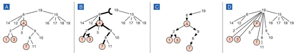
19 6 15 16 17 18 12 4 14 19 2 5 9 1 3 8 10 7 11 19 6 15 16 17 18 12 4 14 19 2 5 9 1 3 8 10 7 11 19 6 15 16 17 18 12 4 14 19 2 5 9 1 3 8 10 7 11 19 6 4 2 9 1 3 8 7 A B C D
Figure 1.A: An example union-find tree with sample queries circled;B: Bolded edges are paths, together with their stopping points, that result from the traversal in Phase I;C: The traversal graphRYrecorded as a result of Phase I; andD: The union-find tree after Phase II, which updates all traversed nodes to point to
their roots.
Algorithm 4:Bulk-FindpU,Sq—find the root inUfor eachsPSwith path compression.
Input:Uis the union find structure. Fori“1, . . . ,|S|,Srisis a vertex in the graph
Output:A response arrayresof length|S|whereresrisis the root of the tree of the vertex Srisin the input.
Phase I:Find the roots for all queries
1: R0Ð xpSrks,nullq : k“0,1,2, . . . ,|S| ´1y
2: F0ÐmkFrontierpR0,Hq,rootsÐ H,visitedÐ H,iÐ0 3: whileRi‰ Hdo
4: visitedÐvisitedYFi
5: Ri`1Ð xpparentrvs,vq : vPFiandparentrvs ‰vy
6: rootsÐrootsY tv : vPFiwhereparentrvs “vu
7: Fi`1ÐmkFrontierpRi`1,visitedq,iÐi`1
Set up response distribution
8: Create an instance ofRDwithRY“R0‘R1‘ ¨ ¨ ¨ ‘Ri
Phase II:Distribute the answers and shorten the paths
9: D0Ð tpr,rq : rProotsu,iÐ0 10: whileDi‰ Hdo
11: For eachpv,rq PDi, in parallel,parentrvs Ðr
12: Di`1ÐŤpv,rqPDitpu,rq : uPRD.allFrompvqandu‰nullu. That is, createDi`1by expanding everypv,rq PDias the entries ofRD.allFrompvqexcludingnull, each inheritingr.
13: iÐi`1
14: Fori“0,1,2. . . ,|S| ´1, in parallel, makeresris ÐparentrSriss 15: returnres
defmkFrontierpR,visitedq: // nodes to go to next
1: reqÐ xv : pv, q PR^
notvisitedrvsy
2: returnremoveDuppreqq
To understand the benefits of path compression, consider a concrete example in Figure 1A, which
shows a union-find treeTthat is typical in a union-find forest. The root ofTisr“19. Suppose we
need to supportfind’s fromu“1andv“7. When all is done, bothfindpuqandfindpvqshould
returnr. Notice that in this example, the paths to the rootuùrandvùrmeet at common vertex
w“4. That is, the two paths are identical fromwonward tor. Iffind’s were done sequentially,
sayfindpuqbeforefindpvq, thenfindpuq—with path compression—would update all nodes on
theuùrpath to point tor. This means that whenfindpvqtraverses the tree, the path to the root
is significantly shorter: at this point, the next hop afterwis alreadyr.
The kind of sharing and shortcutting illustrated, however, is not possible when the find
operations are run independently in parallel. Eachfind, unaware of the others, will proceed all
We fix this problem by organizing the parallel computation so that the work on different “flows”
offinds is carefully coordinated. Algorithm 4 shows an algorithmBulk-Find, which works in two
phases, separating actions that only read from the tree from actions that only write to it:
Phase I: Find the roots for all queries, coalescing flows as soon as they meet up. This phase
should be thought of as running breadth-first search (BFS), starting from all the query nodes S
at once. As with normal BFS, if multiple flows meet up, only one will move on. Also, if a flow encounters a node that has been traversed before, that flow no longer needs to go on. We also need to record the paths traversed so we can distribute responses to the requesting nodes.
Phase II:Distribute the answers and shorten the paths. Using the transcript from Phase I, Phase II makes sure that all nodes traversed will point to the corresponding root—and answers delivered to
all thefinds. This phase, too, should be thought of as running breadth-first search (BFS) backwards
from all the roots reached in Phase I. This BFS reverses the steps taken in Phase I using the trails recorded. There is a technical challenge in implementing this. Back in Phase I, to minimize the cost of recording these trails, the trails are kept as a list of directed edges (marked by their two endpoints) traversed. However, for the reverse traversal in Phase II to be efficient, it needs a means to quickly look up all the neighbors of a vertex (i.e., at every node, we must be able to find every flow that arrived at this node back in Phase I). For this, we design a data structure that takes advantage of hashing and integer sorting (Theorem 1) to keep the parallel complexity low. We discuss our solution to this problem in the section that follows (Lemma 9).
Example: We illustrate how the Bulk-Find algorithm works using the union-find forest from
Figure 1A. The queries to theBulk-Findare nodes that are circled. The paths traversed in Phase I
are shown in panel B. If a flow is terminated, the last edge traversed on that flow is rendered as .
Notice that as soon as flows meet up, only one of them will carry on. In general, if multiple flows
meet up at a point, only one will go on. Notice also that both the flow 1Ñ2Ñ4 and the flow
7Ñ8Ñ9Ñ4are stopped at4because4is a source itself, which was started at the same time as
1and7. At the finish of Phase I, the graph (in fact a tree) given byRYis shown in panel C. Finally,
in Phase II, this graph is traversed and all nodes visited are updated to point to their corresponding root (as shown in panel D).
5.1. Response Distributor
Consider a sequence RY“ xpfromi,toiqyλi“1. We need a data structure RD such that after some
preprocessing of RY, can efficiently answer the query RD.allFrompfqwhich returns a sequence
containing alltoiwherefromi“ f.
To meet the overall running time bound, the preprocessing step cannot take more than Opλq
work andOppolylogpλqqdepth. As far as we know, we cannot afford to generate, say, a sequence of
sequencesRDwhereRDrfsis a sequence containing alltoisuch thatfromi“ f. Instead, we propose
a data structure with the following properties: Lemma 9(Response Distributor)
There is a data structure, response distributor (RD), that from input RY“ xpfromi,toiqyλi“1can be
Oplogλqdepth. Furthermore, ifFis the set of uniquefromi(i.e.,F“ tfromi : i“1, . . . ,λu), then E « ÿ fPF WorkpRD.allFrompfqq ff “Opλq. Proof
Lethbe a hash function from the domain of fromi’s (a subset ofrns) torρs, whereρ “3λ. To
construct anRD, we proceed as follows. Compute the hash for eachfromi usinghp¨qand sort the
ordered pairspfromi,toiqby their hash values. Call this sorted arrayA. After sorting, we know that
pairs with the same hash value are stored consecutively inA. Now create an arrayoof lengthρ`1
so thatoimarks the beginning of pairs whose hash value isi. If none of them hash toi, thenoi“oi`1.
These steps can be done usingintSortand standard techniques inOpλqwork andOppolylogpλqq
depth because the hash values range withinOpλq.
To supportallFrompfq, we computeκ“hpfqand look inAbetweenoκandoκ`1´1, selecting
only pairs whosefrommatches f. This requires at mostOplog|oκ`1´oκ|q “Oplogλqdepth. The
more involved question is, how much work is needed to supportallFromover all? To answer this,
consider all the pairs inRYwithfromi“ f. Letnf denote the number of such pairs. Thesenf pairs
will be gone through by queries looking for f and other entries that happen to hash to the same value
as f does. The exact number of times these pairs are gone through isβf :“#tsPF:hpfq “hpsqu. Hence, across all queries f PF, the total work isřfPFnfβf. ButErβfs ď1`
|F| ρ , so ÿ fPF Ernfβfs ď ´ 1`|F|ρ ¯ ÿ fPF nf ď p1`3λλqλ ď2λ because|F| ďλ andř
fPFnf “λ, completing the proof.
With this lemma, the cost ofBulk-Findcan be stated as follows.
Lemma 10
Bulk-FindpU,SqdoesOp|RY|qwork and hasOppolylogpnqqdepth.
Proof
The Ri’s, Fi’s, and Di’s can be maintained directly as arrays. The roots and visited sets can be
maintained as bit flags on top of the vertices ofUas all we need are setting the bits (adding/removing
elements) and reading their values (membership testing). There are two phases in this algorithm. In
Phase I, the cost of addingFi to visited in iterationi is bounded by |Ri|. Using standard parallel
operations [11], the work of the other steps is clearly bounded by|Ri`1|, includingmkFrontier
becauseremoveDupdoes work linear in the input, which is bounded by|Ri`1|. Thus, the work of
Phase I is at mostOpři|Ri|q “Op|RY|q. In terms of depth, because the union-find tree has depth
at most Oplognq, the whileloop can proceed for at mostOplognqtimes. Each iteration involves
standard operations with depth at mostOplog2nq, so the depth of Phase I is at mostOplog3nq.
In Phase II, the dominant cost comes from expanding Di into Di`1 by calling RD.allFrom.
By Lemma 9, across all iterations, the work caused byRD.allFrom, run on each vertex once, is
expected Op|RY|q, and the depth isOppolylogp|RY|qq ďOppolylogp|RY|qq. Overall, the algorithm requiresOp|RY|qwork andOppolylogpnqqdepth.
5.2. Bulk-Find’s Cost Equivalence to Serialfind
In analyzing the work bound of the improved data structure, we will show that whatBulk-Find
does is equivalent to some sequential execution of the standardfindand requires the same amount
of work, up to constants.
To gather intuition, we will manually derive such a sequence for the sample queries S“
t1,3,4,7u used in Figure 1. The query of4 went all the way to the root without merging with
another flow. But the queries of1 and7 were stopped at 4and in this sense, depended upon the
response from the query of4. By the same reasoning, because the query of3merged with the query
of1(with1proceeding on), the query of3depended on the response from the query of1. Note that
in this view, although the query of3technically waited for the response at2, it was the query of1
that brought the response, so it depended on1. To derive a sequence execution, we need to respect
the “depended on” relation: ifadepended onb, thenawill be invoked afterb. As an example, one
sequential execution order that respects these dependencies isfindp4q,findp7q,findp1q,findp3q.
We can check that by applyingfinds in this order, the paths traversed are exactly what the parallel
execution does asU.findperforms full path compression.
We formalize this idea in the following lemma: Lemma 11
For a sequence of queriesSwith whichBulk-FindpU,Sqis invoked, there is a sequenceS1that is
a permutation ofSsuch that applyingU.findtoS1serially in that order yields the same union-find
forest asBulk-Find’s and incurs the same traversal cost ofOp|RY|q, whereRYis as defined in the
Bulk-Findalgorithm. Proof
For this analysis, we will associate everypparent,childq PRY with a queryqPS. Logically, every
queryqPSstarts a flow atqascending up the tree. If there are multiple flows reaching the same
node,removeDupinsidemkFrontierdecides which flow to go on. From this view, for any nonroot
nodeuappearing inRY, there isexactlyone query flow from this node that proceeds up the tree.
We will denote this flow by ownpuq. All the auxiliary graphs mentioned in this proof are only for
analysis purposes; they are never constructed in the execution of the algorithm.
If a query flow is stopped partway without reaching the corresponding root, the reason is either it
merged in with another flow (viamkFrontier) or it recognized another flow that traversed the same
path before (viavisited). For every queryqthat is stopped partway, letrpqqbe the furthest point in
the tree it has advanced to, i.e.,rpqqis the endpoint of the maximal path inRYfor the query flowq.
In this set up, a query flow whose furthest point isuwill depend on the response from the query
ownpuq. Therefore, we form a dependency graphGdep(“udepends onv”) as follows. The vertices are
all the vertices fromS. For every query flowqthat is stopped partway, there is an arcownprpqqq Ñq.
LetS1 be a topologically-ordered sequence of G
dep. Multiple copies of the same query vertex
can simply be placed next to each other. If we applyU.findserially onS1, then all queries that a
query vertexqdepends on inGdepwill have been called prior toU.findpqq. Because of full path
compression, this means thatU.findpqq will followuùrpqq Ñt (note:rpqq Ñt is one step),
wheret is the root of the tree. Hence, everyU.findpqq traverses the same number of edges as
uùrpqqplus1. As everyRY edge is part of a query flow, we conclude that the work of running
U.findonS1in that order isO
Finally, to obtain the bounds in Theorem 8, we modify Simple-Bulk-Same-Set and
Simple-Bulk-Union (in the relabeling step) to use Bulk-Find on all query pairs. The depth
clearly remainsOppolylogpnqqper bulk operation. Aggregating the cost ofBulk-Findacross calls
fromBulk-UnionandBulk-Same-Set, we know from Lemma 11 that there is a sequential order
that has the same work. Therefore, the total work is bounded byOppm`qqαpm`q,nqq.
6. IMPLEMENTATION AND EVALUATION
This section discusses an implementation of the proposed data structure and its empirical performance, evaluated using a number of large graphs of varying degree distributions.
6.1. Implementation
With an eye towards a simple implementation that delivers good practical performance, we set out to implement the simple bulk-parallel data structure from Section 4. The underlying
union-find data structureU maintains two arrays of lengthn—parentandsizes—one storing a parent
pointer for each vertex, and the other tracking the sizes of the trees. The find and union
operations follow a standard textbook implementation. On top of these operations, we implemented
Simple-Bulk-Same-Set and Simple-Bulk-Union as described earlier in the paper. We use standard sequence manipulation operations (e.g., filter, prefix sum, pack, remove duplicate) from the PBBS library [19]. There are two modifications that we made to improve the performance:
Path Compression:We wanted some benefits of path compression but without the full complexity of the work-efficient parallel algorithm from Section 5, to keep the code simple. We settled
with the following pragmatic solution: Thefindoperations insideSimple-Bulk-Same-Setand
Simple-Bulk-Unionstill run independently in parallel. But after finding the root, each operation traverses the tree one more time to update all the nodes on the path to point to the root. This leads to shorter paths for later bulk operations with clear performance benefits. However, for large minibatches, the approach may still perform significantly more work than the work-efficient solution
because the path compression from one find operation may not benefit other find operations
within the same minibatch.
Connected Components:The algorithm as described uses as a subroutine a linear-work parallel algorithm to find connected components. These linear work algorithms expect a graph representation that gives quick random access to the neighbors of a vertex. We found the processing cost to meet this requirement to be very high and instead implemented the algorithm for connectivity described in Blelloch et al. [3]. Although this has worse theoretical guarantees, it can work with a sequence of edges directly and delivers good real-world performance.
6.2. Experimental Setup
Environment:We performed experiments on an Amazon EC2 instance with20cores (allowing for
40threads via hyperthreading) of2.4GHz Intel Xeon E5-2676 v3 processors, running Linux
3.11.0-19 (Ubuntu 14.04.3). We believe this represents a baseline configuration of midrange workstations available in a modern cluster. All programs were compiled with Clang version 3.4 using the flag
Graph #Vertices #Edges Notes
3Dgrid 99.9M 300M 3-d mesh
random 100M 500M 5randomly-chosen neighbors per node
local5 100M 500M small separators, avg. degree5
local16 100M 1.6B small separators, avg. degree16
rMat5 134M 500M power-law graph using rMat [4]
rMat16 134M 1.6B a denser rMat graph
Table I. Characteristics of the graph streams used in our experiments, showing for every dataset, the total number of nodes (n), the total number of edges (m), and a brief description.
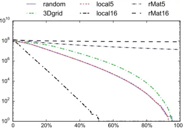
0 20% 40% 60% 80% 100% 100 102 104 106 108 1010
random
3Dgrid
local5
local16
rMat5
rMat16
Figure 2. The numbers of connected components for each graph dataset at different percentages of the total graph stream processed.
-O3. This version of Clang has the Intel Cilk runtime, which uses a work-stealing scheduler known
to impose only a small overhead on both parallel and sequential code. We report wall-clock time
measured usingstd::chrono::high_resolution_clock.
For robustness, we perform three trials and report the median running time. Although there
is randomness involved in the connected component (CC) algorithm, we found no significant fluctuations in the running time across runs.
Datasets:Our experiments aim to study the behavior of the algorithm on a variety of graph streams. To this end, we use a collection of synthetic graph streams created using well-accepted generators. We include both power-law-type graphs and more regular graphs in the experiments. These are graphs commonly used in dynamic/streaming graph experiments (e.g., [14]). A summary of these datasets appear in Table I.
The graph streams in our experiments differ substantially in how quickly they become connected. This input characteristic influences the data structure’s performance. Figure 2 shows for each graph stream, the number of connected components at different points in the stream. The local16 graph becomes fully connected right around the midpoint of the stream. Both rMat5 and rMat16 continue to have tens of millions of components after consuming the whole stream. Note that in this figure, random and local5 are almost visually indistinguishable until the very end.
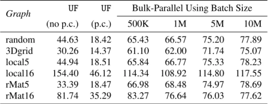
Graph UF UF Bulk-Parallel Using Batch Size (no p.c.) (p.c.) 500K 1M 5M 10M random 44.63 18.42 65.43 66.57 75.20 77.89 3Dgrid 30.26 14.37 61.10 62.00 71.74 75.07 local5 44.94 18.51 65.84 66.77 75.33 78.23 local16 154.40 46.12 114.34 108.92 114.80 117.55 rMat5 33.39 18.47 66.98 68.48 74.97 78.69 rMat16 81.74 35.29 83.27 76.64 76.03 77.62
Table II. Running times (in seconds) on1thread of the baseline union-find implementation (UF) with and without path compression and the bulk-parallel version as the batch size is varied.
Baseline:Because most prior algorithms in this space either focus on parallel graphs or streaming graphs, not parallel streaming graphs, we directly compare our algorithms with sequential union
find implementations (denotedUF), using both the union by size variant and a time-optimal path
compression variant. We note that the algorithm of McColl et al. [14] that works in the parallel dynamic setting is not directly comparable to ours. Their algorithm focuses on supporting arbitrary insertion and deletion of edges, whereas ours is designed to take advantage of the insert-only setting.
6.3. Results
How does the bulk-parallel data structure perform on a multicore machine? To this end, we investigate the parallel overhead, speedup, and scalability trend:
— Parallel Overhead: How much slower is the parallel implementation running on one core compared to a sequential union-find? When running on one core, the parallel implementation should not take much longer than the sequential implementation, showing empirical “work efficiency.”
— Parallel Speedup: How much faster is the parallel version on many cores compared to the parallel version on one core? A good parallel algorithm should achieve a good speedup.
— Scalability Trend:How does the algorithm scale with more cores? Complementing the previous analysis, this helps predict performance on a machine with more cores.
What is the parallel overhead of our implementation?Table II shows the timings for the baseline
sequential implementation of union-findUFwith and without path compression and the bulk-parallel
implementationon a single threadfor four different batch sizes, 500K, 1M, 5M, and 10M. Notice
that the sequential UF implementations do not depend on the batch size. To measure overhead,
we first compare our implementation to union findwithoutpath compression: our implementation is
between1.01x and2.5x slower except on local16, in which the bulk parallel achieves some speedups
even on one thread. This is mainly because the number of connected components in local16 drops quickly to 1 as soon as midstream (Figure 2). With only 1 connected component, there is little work for bulk-parallel after that. Compared to union find with path compression, our implementation, which does pragmatic path compression, shows nontrivial—but still acceptable—overhead, as to be
expected because our solution does not fully benefitfinds within the same minibatch.
How much does parallelization help increase processing throughput?Table III shows the average
throughputs (million edges/second) ofBulk-Unionfor different batch sizes. HereT1denotes the
Graph Usingb“500K Usingb“1M Usingb“5M Usingb“10M T1 T20c T20c{T1 T1 T20c T20c{T1 T1 T20c T20c{T1 T1 T20c T20c{T1 random 7.64 36.87 4.8x 7.51 46.02 6.1x 6.65 60.66 9.1x 6.42 63.90 10.0x 3Dgrid 4.91 27.97 5.7x 4.83 34.97 7.2x 4.18 44.27 10.6x 3.99 45.24 11.3x local5 7.59 38.41 5.1x 7.49 48.32 6.5x 6.64 64.61 9.7x 6.39 64.09 10.0x local16 13.99 78.83 5.6x 14.69 95.57 6.5x 13.94 122.69 8.8x 13.61 122.03 9.0x rMat5 7.47 26.08 3.5x 7.30 34.19 4.7x 6.67 49.92 7.5x 6.35 50.37 7.9x rMat16 19.21 54.94 2.9x 20.88 78.10 3.7x 21.05 143.63 6.8x 20.61 167.68 8.1x Table III. Average throughput (in million edges/second) and speedup ofBulk-Unionfor different batch
sizesb, whereT1is throughput on1thread andT20cis the throughput on20cores.
20physical cores). We also show the speedup factor, as given byT20c{T1. We observe consistent
speedup on all six datasets under all four batch sizes. Across all datasets, the general trend is that the larger the batch size, the higher the speedup factor. This is to be expected since a larger batch size means more work per core to fully utilize the cores, and less synchronization overhead.
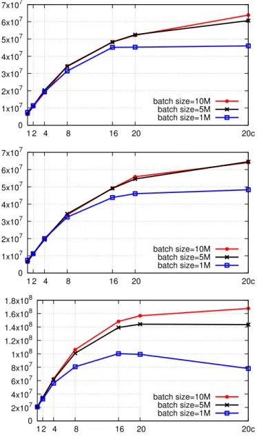
How does the implementation scale with more cores? Figure 3 shows the average throughput
(edges/sec) as the number of threads increases from 1 to20threads, then to40(denoted as20c).
Three different batch sizes were used for the experiments: 1M, 5M and 10M. The top chart show the results on the random dataset, the middle chart on the local16 dataset, and the bottom chart on the rMat16 dataset. Overall, the speedup is significant: with 40 (hyper-) threads, a batch size of
10M edges yields speedups between8–11x. Smaller batch sizes yield somewhat lower speedups.
In general, it is clear thatas the number of threads increases, the average throughput increases for
all batch sizes. An exception to this trend is the rMat16 dataset (bottom) using 1M batch size: the throughput drops slightly when the number of threads increases beyond 20. This is because rMat16 is sparsely connected, as is evident from the high number of components after consuming the whole stream (Figure 2), which in fact has the same order of magnitude as the number of components at the beginning. As a result, in a given minibatch, a large fraction of the edges are links between existing connected components and are discarded quickly at the start of the minibatch, resulting in relatively small work done per minibatch. Hence, at this batch size, there is not enough work to realize additional benefits beyond 20 threads.
7. CONCLUSION
We have presented a shared-memory parallel data structure for the union-find problem (hence, incremental graph connectivity) in the minibatch arrival model. Our algorithm has polylogarithmic parallel depth and its total work across all processors is of the same order as the work due to the best sequential algorithm for the problem. We also presented a simpler parallel algorithm that is easier to implement and has good practical performance.
This still leaves open several natural problems. We list some of them here. (1) In case all edge updates are in a single minibatch, the total work of our algorithm is (in a theoretical sense), superlinear in the number of edges in the graph. Whereas, the optimal batch algorithm for graph
0 1x10⁷ 2x10⁷ 3x10⁷ 4x10⁷ 5x10⁷ 6x10⁷ 7x10⁷ 1 2 4 8 16 20 20c batch size=10M batch size=5M batch size=1M 0 1x10⁷ 2x10⁷ 3x10⁷ 4x10⁷ 5x10⁷ 6x10⁷ 7x10⁷ 1 2 4 8 16 20 20c batch size=10M batch size=5M batch size=1M 0 2x10⁷ 4x10⁷ 6x10⁷ 8x10⁷ 1x10⁸ 1.2x10⁸ 1.4x10⁸ 1.6x10⁸ 1.8x10⁸ 1 2 4 8 16 20 20c batch size=10M batch size=5M batch size=1M
Figure 3. Average throughput (edges per second) as the number of threads is varied from 1 to40(denoted by20cas they run on 20 cores with hyperthreading). The graph streams shown are (top) random, (middle)
local16, and (bottom) rMat16.
connectivity, based on a depth-first search, has work linear in the number of edges. Is it possible to have an incremental algorithm whose work is linear in the case of very large batches, such as the above, and falls back to the union-find type algorithms for smaller minibatches? Note that for all practical purposes, the work of our algorithm is linear in the number of edges, due to very slow growth of the inverse Ackerman’s function. (2) Can these results on parallel algorithms be extended to the fully dynamic case when there are both edge arrivals as well as deletions?
ACKNOWLEDGMENT
This material is based upon work partially supported by the National Science Foundation under grant number IIS 1527541.
REFERENCES
[1] Richard J. Anderson and Heather Woll. Wait-free parallel algorithms for the union-find problem. InProceedings of the 23rd Annual ACM Symposium on Theory of Computing, May 5-8, 1991, New Orleans, Louisiana, USA, pages 370–380, 1991.
[2] Jonathan Berry, Matthew Oster, Cynthia A. Phillips, Steven Plimpton, and Timothy M. Shead. Maintaining connected components for infinite graph streams. InProc. 2nd International Workshop on Big Data, Streams and Heterogeneous Source Mining: Algorithms, Systems, Programming Models and Applications (BigMine), pages 95–102, 2013.
[3] Guy E. Blelloch, Jeremy T. Fineman, Phillip B. Gibbons, and Julian Shun. Internally deterministic parallel algorithms can be fast. InProceedings of the 17th ACM SIGPLAN Symposium on Principles and Practice of Parallel Programming, PPOPP 2012, New Orleans, LA, USA, February 25-29, 2012, pages 181–192, 2012. [4] Deepayan Chakrabarti, Yiping Zhan, and Christos Faloutsos. R-MAT: A recursive model for graph mining. In
Proceedings of the Fourth SIAM International Conference on Data Mining, Lake Buena Vista, Florida, USA, April 22-24, 2004, pages 442–446, 2004.
[5] Thomas H. Cormen, Charles E. Leiserson, Ronald L. Rivest, and Clifford Stein. Introduction to Algorithms (3. ed.). MIT Press, 2009.
[6] Camil Demetrescu, Bruno Escoffier, Gabriel Moruz, and Andrea Ribichini. Adapting parallel algorithms to the W-stream model, with applications to graph problems.Theor. Comput. Sci., 411(44-46):3994–4004, 2010. [7] Camil Demetrescu, Irene Finocchi, and Andrea Ribichini. Trading off space for passes in graph streaming problems.
ACM Transactions on Algorithms, 6(1), 2009.
[8] Joan Feigenbaum, Sampath Kannan, Andrew McGregor, Siddharth Suri, and Jian Zhang. On graph problems in a semi-streaming model.Theor. Comput. Sci., 348(2-3):207–216, 2005.
[9] Hillel Gazit. An optimal randomized parallel algorithm for finding connected components in a graph. SIAM J. Comput., 20(6):1046–1067, 1991.
[10] IBM Corporation. Infosphere streams. http://www-03.ibm.com/software/products/en/ infosphere-streams. Accessed Jan 2014.
[11] Joseph J´aJ´a.An Introduction to Parallel Algorithms. Addison-Wesley, 1992.
[12] Bruce M. Kapron, Valerie King, and Ben Mountjoy. Dynamic graph connectivity in polylogarithmic worst case time. InProceedings of the Twenty-Fourth Annual ACM-SIAM Symposium on Discrete Algorithms, SODA 2013, New Orleans, Louisiana, USA, January 6-8, 2013, pages 1131–1142, 2013.
[13] Fredrik Manne and Md. Mostofa Ali Patwary. A scalable parallel union-find algorithm for distributed memory computers. InParallel Processing and Applied Mathematics, 8th International Conference, PPAM 2009, Wroclaw, Poland, September 13-16, 2009. Revised Selected Papers, Part I, pages 186–195, 2009.
[14] Robert McColl, Oded Green, and David A. Bader. A new parallel algorithm for connected components in dynamic graphs. In20th Annual International Conference on High Performance Computing, HiPC 2013, Bengaluru (Bangalore), Karnataka, India, December 18-21, 2013, pages 246–255, 2013.
[15] Andrew McGregor. Graph stream algorithms: a survey.SIGMOD Record, 43(1):9–20, 2014.
[16] Md. Mostofa Ali Patwary, Peder Refsnes, and Fredrik Manne. Multi-core spanning forest algorithms using the disjoint-set data structure. In26th IEEE International Parallel and Distributed Processing Symposium, IPDPS, pages 827–835, 2012.
[17] Sanguthevar Rajasekaran and John H. Reif. Optimal and sublogarithmic time randomized parallel sorting algorithms.SIAM J. Comput., 18(3):594–607, 1989.
[18] Raimund Seidel and Micha Sharir. Top-down analysis of path compression. SIAM J. Comput., 34(3):515–525, 2005.
[19] Julian Shun, Guy E. Blelloch, Jeremy T. Fineman, Phillip B. Gibbons, Aapo Kyrola, Harsha Vardhan Simhadri, and Kanat Tangwongsan. Brief announcement: the problem based benchmark suite. In24th ACM Symposium on Parallelism in Algorithms and Architectures, SPAA ’12, Pittsburgh, PA, USA, June 25-27, 2012, pages 68–70, 2012.
[20] Julian Shun, Laxman Dhulipala, and Guy E. Blelloch. A simple and practical linear-work parallel algorithm for connectivity. In26th ACM Symposium on Parallelism in Algorithms and Architectures, SPAA ’14, Prague, Czech Republic, pages 143–153, 2014.
[21] Natcha Simsiri, Kanat Tangwongsan, Srikanta Tirthapura, and Kun-Lung Wu. Work-efficient parallel union-find with applications to incremental graph connectivity. InProceedings of the 22nd International European Conference on Parallel and Distributed Computing, pages 561–573, 2016.
[22] Robert Endre Tarjan. Efficiency of a good but not linear set union algorithm.Journal of the ACM, 22(2):215–225, 1975.
[23] M. Zaharia, T. Das, H. Li, T. Hunter, S. Shenker, and I. Stoica. Discretized streams: Fault-tolerant streaming computation at scale. InProc. ACM Symposium on Operating Systems Principles (SOSP), pages 423–438, 2013.