Submitted on 29/October/2011
Article ID: 1923-7529-2012-01-01-24 Guido Russi
~ 1 ~
Estimating the Leverage Effect Using High Frequency Data
1Guido Russi
OXERA Consulting Ltd
Park Central, 40/41 Park End Street, Oxford OX1 1JD, UNITED KINGDOM Tel: +44-(0)1865-253005 E-mail: [email protected]
A
bstract: This paper investigates the dynamics of the leverage effect over time, using high frequency data. By applying Realized Kernel techniques, a more precise estimate of Realized Correlation – compared to standard subsampled estimators of Realized Correlation – is derived. This new measure avoids the so-called Epps effect and permits to observe a level of Realized Correlation significantly different from zero – unlike standard subsampled estimators. Modeling the resulting measure, a deeper insight into the dynamic behavior of Realized Correlation – and hence into the dynamics of leverage effects – is obtained. In particular, this paper studies the behavior of Realized Correlation across the recent financial crisis, to gain a deeper understanding of the factors underlying leverage effects at different stages of the crisis.JEL Classifications: C22, C52, G21
Keywords: Leverage effect, Realized kernels, Realized correlation, Realized variance, Epps effect
1. Introduction and Literature Review
Extensive scholarly attention has been devoted to the so-called “leverage effect”, first theorized by Black (1976), Christie (1982) and Nelson (1991). According to this “leverage effect” theory, a decrease in the level of the stock index leads to a rise in the leverage of listed firms, increasing the risk associated to equity and, consequently, leading to an increase in the level of implied volatility (due to lower strike prices [see Manda, 2010]).
This theory is meant to explain the observed negative correlation between changes in the level of volatility and returns on the stock market: this correlation has been detected empirically in a large number of studies, such as those of Christie (1982), Cheung and Ng (1992), and Duffee (1995), who presented a large body of evidence in support of this apparent “statistical regularity”. More recently, Whaley (2000) who used data on the Chicago Board Options Exchange’s market volatility index (the so-called VIX) and on the S&P 500 provided further evidence in favor of the existence of this negative relationship.2
While a strong consensus appears to back the existence of the negative correlation between implied volatility and stock returns, more conflicting stances characterize academic explanations for this phenomenon. For instance, in 2000, Figlewski and Wang detected a number of anomalies in an empirical study of the leverage effect. These anomalies somewhat undermine the validity of the leverage effect explanation. For example, they observed that variations in the level of outstanding debt (variations that alter the leverage of listed firms) do not trigger volatility changes comparable to those caused by changes in the value of equity (see Figlewski and Wang, 2000).
1
This article is the outcome of work undertaken by the author, independently of Oxera Consulting Ltd. The views expressed in this article—and any errors or omissions—are the author's sole responsibility and should not be attributed to Oxera Consulting Ltd.
2
According to Whaley (2000, p. 17), this negative relationship between the level of the VIX and S&P 500 returns is robust to controls for the nature of the initial shock in the stock market (e.g. threats of wars as opposed to unexpected changes in stock market declines).
Review of Economics & Finance
~ 2 ~
In particular, an alternative “volatility feedback” explanation has managed to gather some consensus among researchers. According to this explanation, volatility is a priced factor. Therefore, if investors anticipate an increase in the level of volatility, the required rate of return on their investments increases. To accommodate this change, prices would have to change. Just like in the leverage effect theory, the outcome of these events would be a rise in the level of volatility and a drop in the stock market returns. However, according to this alternative explanation, the causality is now reversed: changes in expected volatility alter stock market prices and not the other way around (see Bollerslev et al, 2006).
In an attempt to shed some light upon this empirical regularity, subsequent studies have tried to look into the qualitative properties of this negative correlation. For instance, Giot (2002) investigated the relationship between implied volatility and future stock market returns. In other words, he measured the predictive power of VIX as a forecasting variable for stock market returns, finding that high levels of VIX may indicate positive forward looking returns on a long position in the market. A more recent study by Manda (2010), instead, looks at the behavior of VIX returns and returns on the S&P 500 to try and make some inference on the qualitative nature of the leverage effect throughout the 2007/2008 crisis. Manda’s simple exercise suggests that – going from the pre-crisis to the post-pre-crisis period – the relationship between VIX and market returns changes intensity across time, with different types of asymmetries characterizing different stages of the crisis.
With the introduction of new econometric techniques, more sophisticated research on the leverage effect has become possible (see e.g. Glosten et al, 1993). For instance, in an article published in 2003, Simon (2003, p. 15) uses a GJR-GARCH model to investigate the leverage effect during the Internet bubble of the early 2000’s. Sun and Wu (2010), instead, exploit nonparametric copula methods to evaluate extreme tail dependency between the VIX and the S&P 500, finding that this dependency is strong and negative and that the leverage effect is stronger in bearish markets and gradually weakens as markets revert back to their long-run mean (Sun and Wu, 2010, p.2).
As access to high frequency data increased, new studies exploiting this new – and more informative – type of time-series were published. As an example, Bollerslev et al (2007) use high frequency quotes to separate volatility into two different components (splitting the movements in the price series into jumps and continuous paths). One of the conclusions of their paper is that the leverage effect is much weaker for the jump-component of volatility. In a more recent study, instead, high frequency data is used to develop a model that explains expected stock market returns using the difference between implied volatility and realized volatility and introducing restrictions that account for the leverage effect (Bollerslev et al, 2009, p.4467).
Despite this vast body of literature, a thorough knowledge of the temporal structure of this leverage effect – both on a quantitative and on a qualitative level – is yet to be achieved (see, e.g. Bouchaud et al, 2001). To this end, event-based studies, like those of Manda (2010) and Simon (2003) can be particularly informative, in that they expose the dynamic behavior of leverage effects. That is exactly the type of exercise that is attempted in this paper. The purpose of this research, indeed, is to investigate the dynamics of the leverage effect in the years of the recent financial crisis, which was characterized by moments of significant turbulence for financial markets. More specifically, high frequency data on VIX futures and S&P 500 futures is used to assess evidence of the leverage effect from 2007 to 2010. Multiple studies have exploited high frequency datasets to study this effect (cfr De Pooter et al, 2006 and Bollerslev et al, 2006), but, to the best of the author’s knowledge, no study has yet attempted to apply Realized Kernel techniques to this richer type of datasets. Realized Kernel estimators, first proposed by Barndorff-Nielsen et al (2008a), represent a method to compute Integrated Covariances that are robust to the noise that might affect the quote data. This estimator is also guaranteed to be positive semi-definite and can also handle
non-~ 3 non-~
synchronous trading (Barndorff-Nielsen et al, 2008b, p. 2). In other words, Realized Kernels, when appropriately parametrized, make a more efficient use of information (see Gatheral and Oomen, 2010, p 279). In addition, the adoption of Realized Kernel techniques permits to model volatility – which is inherently a latent variable – using observable proxies.
In this empirical analysis, Realized Kernels are used to compute Realized Correlation between VIX futures and S&P 500 futures. The analysis of Realized Correlation represents a method to gain useful insights into the dynamics of leverage effects, even in the absence of a sound theoretical understanding of the causality link that underpins this phenomenon.3
To sum up, this paper attempts to enquire into the time-series dynamics of leverage effects during the 2007/2008 financial crisis, by computing Realized Correlation between VIX futures and S&P 500 futures every day. In applying more recent – and more efficient – econometric techniques, the hope is that of acquiring an in-depth understanding of the time dynamics of leverage effects. Developing a better comprehension of these dynamics may indeed be useful to understand, for example, the role played by investors’ sentiment in the chain of events that propelled the 2007/2008 crisis. Furthermore, a more accurate description of the qualitative and quantitative properties of leverage effects may be exploited by financial practitioners to design new investment strategies. Indeed, incorporation of leverage effects into portfolio diversification strategies has been attempted in the past (see Szado, 2009) and additional insights into this empirical regularity may foster further research in the field.
The paper therefore proceeds as follows. Section 2 provides a general description of the dataset utilized by the author, outlining the main features of the assets for which Realized Correlation is computed. In Section 3, instead, a description of the main steps of the algorithm adopted to account for some of the primary sources of market noise in our dataset is given. Next, Section 4 describes the actual computation of Realized Correlation and of the modeling of this newly obtained variable. Finally, Section 5 describes the results obtained from the exercises performed – trying to assess the evidence gathered – and concludes.
2. Description of the Dataset
In an approach consistent with that of Simon and Wiggins (2001), high-frequency tick-by-tick S&P 500 futures data and high-frequency tick-by-tick VIX futures data were used to perform this investigation. The main reason for preferring futures data to index data, especially for the S&P 500, is that indexes are calculated from the last transaction price of each of the stocks in the index. Since not all stocks trade every minute, this may result in an infrequent trading problem and bias (Martens, 2002, p. 500).
2.1 VIX and VIX Futures
VIX, the Chicago Board Options Exchange’s market volatility index, is an index that captures the market’s expectation of future volatility, using a portfolio of S&P 500 options (rather than stocks). It is regarded among academics and practitioners as an indicator of investors’ sentiment and it has been described as an “investor fear gauge” (Whaley, 2000, p.12). The original version introduced by Whaley (1993) was based on the S&P 100. The current version of the VIX, based on the S&P 500, was instead introduced in 2003. The VIX index attempts to capture 30-day expected volatility and is computed on a portfolio of near- and next- term call and put options (corresponding usually to the first and second months of the S&P contract). Options that do not have at least one
3
As outlined in previous paragraphs, both the leverage effect theory and the volatility feedback theory are still regarded as potential explanations for the leverage effect.
Review of Economics & Finance
~ 4 ~
week to expiration are not included in the portfolio, to avoid pricing anomalies that may arise as the expiration date gets closer. Instead, when near-term options have less than 9 days to expiration, the VIX rolls to the second and third months of the S&P contract (CBOE, 2003).
In this empirical analysis, VIX futures, as opposed to spot VIX, have been used. One of the main differences between VIX futures and spot VIX is that, unlike VIX futures, spot VIX is not directly investable at present.4 Also, VIX futures are not simply a measure of the expected volatility of the S&P index: they also reflect expectations on the expected one-month volatility at a specific point in time in the future. From a theoretical perspective, VIX futures should converge to spot VIX as the expiration date gets closer. However, in practice, significant anomalies in this theoretical convergence process are possible prior to expiration (see Szado, 2009, p.73). Finally, VIX futures are generally characterized by lower volatility than spot VIX, partly because of the mean reverting nature of volatility (Szado, 2009, p.73).
It is important to point out that VIX futures, traded on the CBOE Futures Exchange, were introduced only in 2004. This inception date is quite important in this study because the dataset at hand spans the years between 2006 and 2010. While, in general, the level of liquidity appears to be reasonable for this window of time, periods of low levels of trading activity are still observed in 2006.5
For this empirical investigation, data on the VIX futures was downloaded from the CBOE Futures Exchange. VIX futures prices went from January 1, 2006 to December 31, 2010.6
The asset is traded between 8:30 am and 3:15 pm, Chicago time,7 and the contract size is 1000$ times the VIX. The minimum price fluctuation is 0.05 index point, equivalent to 50$ per contract. Contracts exist for every month of the year (CBOE, 2011) and the commencement of trade and expiration of each contract occur on different dates.
The contract size was changed on March 26, 2007 (see CBOE, 2007) and consequently data-points which predate this event require adjustments. In particular, for the period leading up to this date, prices have been divided by a factor of 10 to maintain a uniform contract size across the whole dataset.
The dataset contains overall 2,218,485 data-points, i.e. 9188 trading days. The table below displays the mean, the maximum and minimum value and a set of percentiles for the time-series of prices, as well as for the daily volume and the daily number of transactions.
Table 1 VIX futures dataset prior to clean-up procedure
Variable Min Max Mean 5th percentile 25th percentile 50th percentile 75th percentile 95th percentile Price 3.45 300 26.9231 18.25 22.65 25.85 29.85 41.1 Daily Volume 1 29982 885.5337 4 40 190 743 4419.1 Daily Number of Transactions 1 11733 241.4546 2 12 50 211 1130.2 4
However, VIX is a portfolio of options. Consequently, it is possible to invest in this asset through purchases (or short sales) of these options.
5
See Section 3.
6
Summary statistics for the original dataset are reported in an Appendix which may be requested directly from the author.
7
These are the regular trading hours. Transactions can actually take place between 7:20 am and 8:30 am as well (extended trading hours). See CBOE (2011).
~ 5 ~
The first months of the dataset are still characterized by low levels of trading activity (as approximated by the number of transactions and trading volume).8 Hence, it will be important to account for this factor in subsequent Sections of this work.
2.2 S&P 500 Futures
This analysis relies on data on E-mini S&P 500 futures, rather than “ordinary” S&P 500 futures. E-mini S&P 500 futures represent a relatively new instrument to trade S&P 500 futures, offering investors an alternative to traditional floor-trading futures. These E-mini futures for the S&P 500 were first introduced on September 9, 1997 and since their inception they have been growing rapidly on the CME (Chung and Chiang, 2006, p. 276). The innovative element of these contracts was their fully electronic nature and their smaller size (50$ times E-mini S&P 500 futures price [CME Group, 2011]), potentially attracting investors with smaller margins. E-mini futures are traded almost around the clock on the Chicago Mercantile Exchange9 and these contracts expire four times annually.
The reason for preferring E-mini S&P 500 futures to floor-trading S&P 500 futures is that these electronic contracts exhibit features that make them potentially more suitable to our analysis. In the paragraphs below, a brief description of these characteristics is presented.
While floor-trading futures and E-mini futures are similar in many ways (both contracts are based on the same index, both contracts have the same expiration date, both contracts are cash-settled to the same index value on quarterly expirations and both contracts settle daily to the regular index futures contracts’ settlement price [Ates and Wang, 2005, p.687]), they differ in many features. First and foremost, the floor-trading S&P 500 futures contract multiplier is five times the contract multiplier of the corresponding regular futures and E-mini contracts are traded fully electronically (Ates and Wang, 2005, p. 687).
Also, as outlined by several studies, E-mini futures have several different desirable features (Chung and Chiang, 2006, p. 276):10
“the nature of their small size at lesser margins” “the effective anonymity of traders”
“improved pricing transparency”
“increased speed of transaction execution” “timely reporting of order fills”
Finally, as suggested by Hasbrouck (2003) and Domowitz and Steil (1999), electronic markets offer in general a level of liquidity comparable to that of ordinary floor markets, yet entailing lower costs. This potential opportunity for cost savings may lie at the heart of the observed shift from floor-traded futures trading to E-mini futures trading (Chung and Chiang, 2006, p. 276).
Because of the features listed above, it would therefore seem that E-mini futures markets may be characterized by more informative prices than floor-trading futures markets.11 This constitutes a further reason for preferring E-mini futures over ordinary floor-trading futures.
8
This can be easily inferred from the summary statistics reported in the Appendix available from the author.
9
E-mini futures are traded almost 24 hours a day from Monday to Thursday, with only a 30-minute shutdown period between 4:30 and 5:00 pm. In addition, these contracts are traded from 0:00 am to 3:15 am on Fridays and from 3:15 to midnight on Sundays (see CME Group, 2011).
10
Review of Economics & Finance
~ 6 ~
One last argument in favor of the utilization of E-mini futures instead of floor-trading futures is that the reliance of E-mini contracts on an electronic system to execute all transactions implies that all trading activity occurs in the absence of human intervention (see Ates and Wang, 2005, p. 687). This aspect may be extremely beneficial to this empirical investigation, since it affects the amount of typos present in the dataset and, hence, the overall quality of the data.
On a closing note, it is still important to bear in mind that arbitrage activities between the two types of contracts ensure that the two assets exhibit a very high level of correlation (see Chung and Chiang, 2006, p. 276). Consequently, the choice of E-mini futures as opposed to floor-trading futures should not lead to significant losses of information.
The dataset spans the period going from January 2, 2006 to December 31, 2010.12 The minimum price fluctuation is 0.25 index points (12.50$ per contract). Transaction records are available for a total of 9188 trading days (258,630,003 data-points) and further information on the mean, maximum and minimum values of the dataset (together with other relevant measures) is contained in Table 2.13
Table 2 VIX futures dataset prior to clean-up procedure
Variable Min Max Mean 5th percentile 25th percentile 50th percentile 75th percentile 95th percentile Price 0 1618.25 1135.87 - - - - - Daily Volume 0 5829444 477600.2 0 2 611 685896 2415187 Daily Number of Transactions 1 1356921 53458.04 1 34 663.5 41359 325604.2
The level of liquidity of E-mini futures is quite different from that of VX futures.14 In particular, unlike VIX futures, E-mini contracts display large trading volumes already at the beginning of the dataset.
3. Preliminary Cleaning
Prior to proceeding with the actual data analysis, it is important to prepare the dataset, by performing some preliminary cleaning on the high frequency data. Specifically, four main issues need to be addressed: (i) multiplicity of contracts traded at each point in time for each of the two assets (and need to identify “roll-over” dates), (ii) different regular trading hours for each of the two contracts at hand, (iii) uneven levels of liquidity across time, especially for the VIX futures contracts and (iv) presence of typos and outliers in the dataset.
The issues above are dealt with in the subsequent Subsections. 3.1 Roll-over Dates
The first issue that needs to be addressed is the fact that multiple contracts with different maturities are traded at each point in time, both for the E-mini futures (ES contracts) and for the VIX futures (VX contracts). It is therefore important to choose what contract to use each day for the 11
In 2003, Hasbrouck demonstrated that price discovery for the U.S. equity index market is dominated by electronic markets. See Hasbrouck (2003, p. 2397).
12
Summary statistics are reported in the Appendix available from the author.
13
Due to the extremely large size of the E-mini futures dataset, percentiles for the time-series of prices could not be estimated.
14
~ 7 ~
computation of the Realized Correlation. In doing so, one must take into account the fact that, upon expiration of a future, investors roll over their contracts, taking equivalent positions in other futures expiring at a later date. Therefore, as the expiration date of a future contract gets closer, trading activity shifts at an increasing pace towards a different contract with a longer maturity.15
While not trivial, the solution to this problem for ES futures is simplified by the observed structure of the transactions. Indeed, a few days before the expiration date of an ES future, the volume of transactions of that contract starts dropping in an almost perfect monotonic way. In the same time period, the volume of transactions of the ES future with the next-shortest maturity starts increasing almost in a perfectly monotonic way as well. Consequently, to maximize the overall volume of transactions (and therefore to ensure that the series of prices used is liquid enough), the choice of roll-over dates for ES futures was the following:
Compute the day in which the daily volume of transactions on the “expiring” contract drops below the daily volume of transactions for the contract with the next-shortest maturity.16
Use the day before this date as the roll-over date.17
This solution, however, cannot be easily replicated on VX futures: the structure of transactions for this type of assets is indeed much different from that of ES futures. As a matter of fact, the decay in the volume of transactions prior to the expiration of a VX future does not occur in a monotonic away. Likewise, the corresponding increase in the volume of transactions for the next-shortest-maturity future is not monotonic either. As a result, if the rule described above were to be used for VX futures, multiple crossing days would be identified in the first step and no unique roll-over date would be determined (in the absence of an appropriate selection criterion).
Thus, the following alternative procedure has been adopted:
For each VX contract, the time-series of the daily volume of transactions for that contract and for the next-shortest-maturity contract were set aside.
An optimization exercise was performed: the date that would maximize the overall volume of transactions – if used as roll-over date – was determined.18
This date was selected as roll-over date.
Once roll-over dates were selected, a total of 1259 trading days for VX futures and 1552 trading days for ES futures remained to be analyzed.19
3.2 Liquidity Adjustments
The second step in cleaning up the data is ensuring that all trading days exhibit sufficient levels of liquidity. Indeed, trade size differentials and the informational content of prices have been described as two components of market microstructure noise (Ait-Sahalia and Yu, 2008, p. 3). Also,
15
The existence of a maturity effect (whereby volatility increases as the expiration date gets closer) for future contracts is currently debated. However, since evidence of this effect for financial futures appears to be rather weak (see Moosa and Bollen, 2001, 693), the issue is ignored in this paper.
16
Hereinafter, the crossing day.
17
In other words, the prices of the “expiring” contract were used for our computations up to and including the roll-over date.
18
After optimizing for the first future contract, a small correction had to be applied to this algorithm. From the second future on, data for the “expiring” contract that predates the previous rollover date was eliminated. This correction is necessary to ensure that rollover dates are – in a chronological sense – an ordered sequence.
19
These values will be slightly lower once the other cleaning procedures – including the identification of common trading days – are implemented.
Review of Economics & Finance
~ 8 ~
the potential link between market liquidity and market efficiency has been suggested in multiple academic works (see, e.g. Muranaga and Shimizu, 1999).
Hence, to avoid illiquid trades and to achieve a minimal level of liquidity across the time series, trading days with a volume smaller than 100 (for the VX series) and 1,000,000 for ES were removed.20 This procedure resulted in the removal of 531 trading days for the ES series and four trading days for the VX series.21 The days excluded are days with low levels of trading activity, such as days leading up to or following US bank holidays.22
Once this operation was performed, a list of trading dates common to both E-mini futures and to VIX futures was created. This step was justified by the need to have prices for both of the series on each trading day analyzed. After this final operation, 1021 trading days per series remained for our empirical analysis.
3.3 Common Trading Hours
A further issue that deserves some attention is the difference in regular trading hours between E-mini futures contracts and VIX contracts. As previously outlined, ES futures are traded almost 24 hours a day23 on the CME Globex platform, whereas VIX futures are traded from 8:30 am to 3:15 pm on the CBOE Futures Exchange. To compute Realized Correlation, only transactions executed in common regular trading hours can be utilized.
Hence, all tick data outside the 8:45 am – 3:00 pm window has been excluded from this investigation. The reason for choosing this window instead of a broader 8:30 am – 3:15 pm window is that a vast body of empirical studies documents increased return volatility and trading volume at the open and close of stock markets (cfr Chan et al, 2000, p. 496 and Wood et al, 1985, p. 738). As a result, a 15-minute cushion both at the open and at the close may strike a good balance between avoiding abnormal trading activity in the market and preserving enough data-points to be able to perform estimation procedures in a consistent way.
While performing this clean-up procedure, trading days exhibiting less than 5 ticks (within the 8:30 am – 3:00 pm window) were removed from the dataset, to ensure that enough data-points would be available each day to compute Realized Correlation. Once this operation was performed, though, a further exclusion of all data-points predating January 1, 2007 had to be enacted. Indeed, periods of excessively low liquidity (for VX contracts) resulted in extended windows of days where no Realized Correlation could be computed. Upon completion of all of these operations, the dataset was composed of 917 trading days per series.
20
A similar procedure is adopted by Lu and Zhu in their 2009 empirical investigation (Lu and Zhu, 2009, p. 238). The values of 100 and 1,000,000 are arbitrary but were chosen because they permitted to get rid of illiquid trading days, while at the same time preserving a sufficient amount of data to permit consistent estimation in the subsequent stages of the study. At a first glance, 1,000,000 transactions may appear to be a high threshold, since the mean daily volume is 477,600.2 in the original dataset. However, once roll-over dates were identified and only the most liquid assets were considered every trading day, the mean daily volume significantly increased, making 1,000,000 transactions a reasonable threshold for our analysis.
21
Actually, the amount of trading days of VIX futures that were ruled out by this procedure is much larger. Indeed, when common trading days of the two assets will be identified at a later stage, many more trading days of VIX futures will be excluded.
22
For instance, a proportionally large share of the excluded days (116 out of 531) is in the months of December and January, around Christmas and New Year.
23
~ 9 ~ 3.4 Typos and Outliers
Once a time series of contract names listing what prices to use on each date has been developed and appropriate windows of time have been selected to identify the data-points relevant to our analysis, intra-daily cleaning of the data has to be performed. Indeed, as argued by Barndorff-Nielsen et al (2009, p. 7),“[t]he realized kernel and related estimators “treat all observations equally” and a few outliers can severely influence these estimators.” Because of this, careful preliminary cleaning of data may significantly improve volatility estimators.
Accordingly, three operations were performed on the dataset.
First, all transactions with a price equal to or smaller than zero were removed from the dataset.24 This type of mistakes was found in 763 trading days for the E-mini futures.25
Next, high frequency data was scanned in search of transactions with identical timestamps. However, in the whole time period under analysis,26 no two transactions with exactly the same timestamp were found, in either of the futures time-series.
Finally, to identify observations that appear to be incompatible with the prevailing market trading activity, four different noise measures were computed for each trading day:27
, where S is the set of nonzero returns and v is the dimension of S.
This measure, similar to that proposed by Barndorff-Nielsen et al (2009, p. 7),28 captures the daily number of observations that deviate by more than 5 mean absolute deviations from a rolling centered median of 20 observations.29
Once these four measures were computed, a list of noisy dates was created, using those trading days that (i) were characterized by a strictly positive value of P or (ii) ranked in the first 50 when trading days were classified by either or N. This list comprised 69 trading days – for the VIX futures – and 89 trading days – for the S&P 500 futures.
After scanning the trading days contained in this list, however, all observations seemed to be compatible with the dominant market activity. This was probably due to the cleaning procedures previously implemented, which removed trading days with lower liquidity and lowered the likelihood of encountering typos and outliers.
24
In accordance with rule P2 presented by Barndorff-Nielsen et al (2009, p. 7).
25
No non-positive prices were found in the VIX futures price series.
26
Each trading day, only the 8:30 am -10:30 am window of observations was checked.
27
In the list below – and throughout the entire article – the following notation is used: rt represents the
returns on a specific asset at time t, pt represents the price of a specific asset at time t and I(∙) is an
indicator function.
28
The modifications applied to the original version of the rule are due to the different size of our dataset (using a larger window for the rolling median would have resulted in a large number of transactions being excluded from this check).
29
Review of Economics & Finance
~ 10 ~
Once all of the four issues addressed in the Subsections above were addressed, a final clean dataset was ready for the estimation stage of this investigation.30 978,207 data-points remain for the VX price series and 231,694,318 for the ES series.
Figure 1 and Figure 2, instead, depict the daily trading volume for the two assets. Figure 3 and Figure 4 on page 11, display the logarithm of the daily number of transactions and of the daily trading volume for the two types of contracts.
Figure 1 Clean S&P 500 futures dataset – daily volume
Figure 2 Clean VIX futures dataset – daily volume
30
~ 11 ~
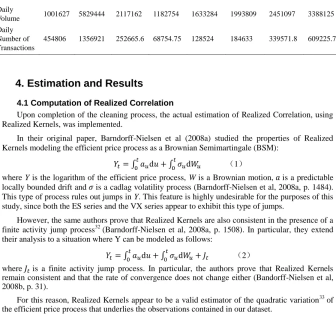
Finally, Tables 3 and 4 on page 12, represent the updated version of Table 1 and Table 2, reflecting the outcome of the whole clean-up procedure.31 One of the most evident changes is that prices now fluctuate in more reasonable bands (e.g. previously, the minimum ES price was 0) and that the mean volume and number of transactions has increased for both assets, consistently with the purpose of this clean-up procedure.
Figure 3 Clean dataset - daily trade volume (logarithm)
Figure 4 Clean dataset - daily number of transactions (logarithm)
31
Since the size of the ES price series is still extremely large, estimation of the percentiles reported in Table 1 was not computationally feasible.
Review of Economics & Finance
~ 12 ~
Table 3 VIX futures dataset after clean-up procedure
Variable Min Max Mean 5th
percentile 25th percentile 50th percentile 75th percentile 95th percentile Price 10.8 72.8 26.9149 18.35 21.8 25.15 29.5 44.58 Daily Volume 215 28104 3811.06 617.85 1264.75 2508 4926 11174.8 Daily Number of Transactions 46 11733 1066.75 152.05 445 712 1317.5 2850.45
Table 4 E-mini futures dataset after clean-up procedure
Variable Min Max Mean 5th
percentile 25th percentile 50th percentile 75th percentile 95th percentile Price 665.75 1586.75 1122.2 - - - - - Daily Volume 1001627 5829444 2117162 1182754 1633284 1993809 2451097 3388125 Daily Number of Transactions 454806 1356921 252665.6 68754.75 128524 184633 339571.8 609225.7
4. Estimation and Results
4.1 Computation of Realized Correlation
Upon completion of the cleaning process, the actual estimation of Realized Correlation, using Realized Kernels, was implemented.
In their original paper, Barndorff-Nielsen et al (2008a) studied the properties of Realized Kernels modeling the efficient price process as a Brownian Semimartingale (BSM):
(1)
where Y is the logarithm of the efficient price process, W is a Brownian motion, is a predictable locally bounded drift and is a cadlag volatility process (Barndorff-Nielsen et al, 2008a, p. 1484). This type of process rules out jumps in Y. This feature is highly undesirable for the purposes of this study, since both the ES series and the VX series appear to exhibit this type of jumps.
However, the same authors prove that Realized Kernels are also consistent in the presence of a finite activity jump process32 (Barndorff-Nielsen et al, 2008a, p. 1508). In particular, they extend their analysis to a situation where Y can be modeled as follows:
(2)
where is a finite activity jump process. In particular, the authors prove that Realized Kernels remain consistent and that the rate of convergence does not change either (Bandorff-Nielsen et al, 2008b, p. 31).
For this reason, Realized Kernels appear to be a valid estimator of the quadratic variation33 of the efficient price process that underlies the observations contained in our dataset.
32
A finite activity jump process is a process with “a finite number of jumps in any bounded interval of time” (Barndorff-Nielsen et al, 2009, p. 2).
~ 13 ~
To estimate Realized Covariance under this approach, the formula presented by Barndorff-Nielsen et al (2009, p. C3) is applied:
(3)
where k(∙) is a kernel weight function, X is the vector of noisy observations of Y, x is the vector of high-frequency returns, n is the number of high-frequency returns available and H is the chosen bandwidth. For this study, a non-flat-top Parzen kernel was used34 and the bandwidth selection procedure outlined by the same authors35 was implemented each time.
The result of this estimation procedure is a time-series of Realized Kernels, from which a time series of Realized Correlations is derived.36 Figure 5 plots the behavior of the estimated (negative) Realized Correlation across time.
Figure 5 Estimated Negative Realized Correlation (from Realized Kernel)
As predicted by the theory, (negative) Realized Correlation is usually negative (positive). Periods in which the sign of (negative) Realized Correlation actually reverses can be easily identified in the plot. For instance, in the months of January 2007, December 2007 and December 2008, positive values for the Realized Correlation can be observed. Positive correlation implies that leverage effects are not in place. However, it is not possible to exclude that this feature is caused by increased levels of noise in these periods of festivities, where trading activity is low.37
As a robustness check, Realized Correlation was also computed by calculating Realized Covariance through the standard formula that does not rely on kernels. In order to exploit all the 33
Quadratic variation is the sum of the integrated covariance plus the outer product of the jumps (Anderson and Liao, 2011, 14).
34
The choice of a Parzen kernel, as opposed to other kernels such as the more famous Bartlett kernel, is due to a desire to develop a consistent estimator. As explained by Barndorff-Nielsen et al (2009, p. C3) the Bartlett kernel does not guarantee consistency and is therefore not adopted in this context.
35
The bandwith estimator developed by Barndorff-Nielsen et al is an empirically tractable estimator and, as explained by the same authors, it is ‘optimal in an asymptotic MSE sense’ (Barndorff-Nielsen et al, 2009, p. C5).
36
Realized Correlation is obtained, at each point in time, as the ratio of the Realized Covariance divided by the square root of the product of the Realized Variances of the two price series.
37
Review of Economics & Finance
~ 14 ~
information contained in the dataset, subsampling was used in computing Realized Correlation. To this end, 1-minute, 5-minute, 10-minute, 15-minute and 20-minute returns were calculated. The outcome of this robustness check is reported in Figure 6. From these plots, the so-called Epps effect emerges in a rather visible way. The Epps effect consists in the correlation among returns getting smaller as the window over which the returns are measured gets smaller (Epps, 1979).
It is easy to see how the 1-minute Realized Correlation series does not appear to be overly noisy but, because of this Epps effect, the whole plot seems to crash onto the x-axis. As the frequency with which returns are measured decreases, the Epps effect appears to drive the gradual shift of the Realized Correlation away from the x-axis. However, as this frequency decreases, the microstructure noise that affects the standard subsampled version of the Realized Correlation increases, leading to a more imprecise plot. This effect prevents standard subsampled versions of the Realized Correlation from detecting a level of Realized Correlation significantly different from zero, regardless of the frequency adopted to measure returns.
Negative Realized Correlation from Standard Subsampled Realized Covariance (1-min returns)
Realized Correlation from Standard Subsampled Realized Covariance (5-min returns)
Realized Correlation from Standard Subsampled Realized Covariance (10-min returns)
Realized Correlation from Standard Subsampled Realized Covariance (15-min returns)
~ 15 ~
Realized Correlation from Standard Subsampled Realized Covariance (20-min returns)
Negative Realized Correlation (from Realized Kernel)
Figure 6 Standard Subsampled Realized Correlations and Epps effect (Realized Kernel Correlation shown for comparison)
Overall, it would therefore seem that the kernel version of the Realized Correlation is indeed the measure least affected by microstructure noise and the only one capable of capturing the actual sign of the Realized Correlation (and hence the leverage effect). Therefore, the Multivariate Realized Kernel is selected for the final part of this investigation.
Once an accurate measure of Realized Correlation was generated, a model that could possibly explain the behavior of this variable over time (and hence the dynamics of the leverage effect) was developed.
4.2 Estimation of Potential Regressors
Prior to engaging in the actual model selection procedure, a number of measures were extracted from the dataset, so as to single out a set of regressors that could be used in the subsequent model-fitting procedures.
The variables chosen to this end were:
The series of returns on ES and VX contracts, computed using the closing price (the 3:00 pm price). These two variables were labeled as Ret_ES and Ret_VX.
The percentage of jumps in the Realized Variance of each of the two assets.
Jumps for each asset were measured as the difference between Realized Variance and Bipower Variation. Barndorff-Nielsen and Shephard (2004) developed Bipower Variation while trying to decompose Realized Variance into a jumps-component and a continuous-path component. Since Bipower Variation represents the continuous-continuous-path component, the difference between Realized Variance and Bipower Variation represents the jump-component of total volatility in any given trading day. Bipower Variation and Realized Variance were computed using 5-minute returns and subsampling techniques, so as to exploit the full informational content of the dataset.
The percentage of jumps in the Realized Variance was than computed simply as the ratio between the jump-component and the Realized Variance at each point in time. An indicator function was inserted to control for noise and to ensure that these percentages would always be positive.38
38
Negative values are driven by market noise and, as a consequence, inserting this indicator function should not affect – or could possibly even improve – the reliability of the dataset.
Review of Economics & Finance
~ 16 ~
These two variables, labeled as PJRVES and PJRVVX, were therefore computed according to the following formula:
(4)
where RV and BV are the levels of Realized Variance and Bipower Variation on each asset. The levels of Realized Variance for each of the two assets: RV_ES and RV_VX. These were
simply obtained in the previous step, implementing a subsampled Realized Variance estimator on 5-minute returns.
Plots of these variables are reported as in Figures 7 to 12 on three pages.
Figure 7 Returns on S&P 500 futures (closing prices)
~ 17 ~
Figure 9 Percentage of Jumps in Realized Variance - S&P 500 futures
Figure 10 Percentage of Jumps in Realized Variance - VIX futures
Review of Economics & Finance
~ 18 ~
Figure 12 Annualized Realized Volatility (%) - VIX futures 4.3 Stationarity Check on Regressand and Regressors
Once these variables were computed, Augmented Dickey-Fuller tests (Dickey and Fuller, 1979) were performed to check for the stationarity of each of the 7 series (Realized Correlation and the six regressors listed above). Results for these tests are reported in Table 5. As can be clearly observed, non-stationarity is rejected in all cases, except for the test on Realized Correlation without deterministic trends. However, since at least a slight time-trend can be detected in the Realized Correlation plot, non-stationarity was ruled out for this variable as well.
Table 5 Augmented Dickey-Fuller tests on the variables under consideration (p-values)
Asset name No deterministic
trends Constant Time trend
Constant and time trend Realized Correlation 0.2147 0 0 0 PJRVES 0 0 0 0 PJRVVX 0 0 0 0 Realized Variance - ES 0 0 0 0 Realized Variance - VX 0 0 0 0 Daily Returns – ES 0 0 0 0 Daily Returns - VX 0 0 0 0 4.4 Model Selection
Before fitting any model, all of the variables presented above were studentized, so as to facilitate the interpretation of regression coefficients in the final model. Indeed, by dividing each variable by its standard deviation, it is possible to report standardized (or beta) coefficients. These coefficients capture the change (measured in standard deviations) in the regressand following a one-standard-deviation change in the relevant regressor (Schoreder et al, 1986, p. 32).
To begin the modeling stage of this study, a baseline model was estimated:
(5)
~ 19 ~
This baseline model is inspired by the Heterogeneous Autoregressive model proposed by Corsi (2009, p. 193). The interesting feature of this baseline model is that it captures the long memory behavior of volatility. In particular, the independent variables of the regression control for daily, weekly and monthly persistence in the series.
Estimates for the baseline model are reported in Table 6. The only variable to actually exhibit a statistically significant coefficient is the 22-day moving average, suggesting that substantial persistence (on a monthly basis) characterizes Realized Correlation. In particular, since the coefficient on this variable is positive, a negative level of Realized Correlation (consistent with the presence of leverage effects in the market) would tend to revert back to zero over time.
Table 6 Baseline HAR-type model Regression results – Predicting Realized Correlation
0.0383 (0.0508) 0.1096 (0.1082) 0.7333 (0.1020)*** 894 -0.3455 0.2276 -0.3241 0.2250 -0.3373 0.8395 295.098 -1135.11 0.0000
Notes: 1. The table reports regression coefficients followed by standard errors in parentheses. 2. *, **, *** indicate statistical significance at the 10%, 5% and 1% levels, respectively. 3. The model includes an intercept which is not reported.
To understand the explanatory power of each of the potential regressors computed previously – both individually and jointly – an automated search using two Information Criteria, AIC and BIC, was performed. In particular, lagged values of the six regressors identified in the previous Section were combined in every possible way and the resulting models were estimated. A total of 64 models were fit39 and the models with the lowest values of AIC/BIC were selected. The best model selected by AIC is described in Table 7 below.
Table 7 AIC-optimal model Regression results – Predicting Realized Correlation
0.0312 (0.4974) -0.2946 (0.0751) *** -0.0504 (0.0038) *** -0.0577 (0.0324) * -0.1076 (0.0095) *** 0.1188 (0.2841) 0.1309 (0.0009) *** 894 -0.3505 0.2383 -0.3076 0.2323 -0.3341 0.8355 320.109 -1130.77 0.0000
Notes: 1. The table reports regression coefficients followed by standard errors in parentheses. 2. *, **, *** indicate statistical significance at the 10%, 5% and 1% levels, respectively. 3. The model includes an intercept which is not reported.
39
Review of Economics & Finance
~ 20 ~
The BIC, instead, selected the baseline HAR-type model, the most parsimonious one. This outcome was to be expected, since BIC places larger penalties on models with a greater number of explanatory variables. It is important to point out that this result may constitute important evidence that the variables selected as potential regressors may actually not add much explanatory power to a simple model like that selected by the BIC.
Nevertheless, since the purpose of this analysis is that of understanding what variables actually affect Realized Correlation and through what channels they do so, greater emphasis should perhaps be put on the models selected by AIC (despite the loss in terms of parsimony). For this reason, the remaining part of this analysis focuses only on the model selected by the AIC.
Looking at the model selected by the Akaike Information Criterion, several important aspects are detected:
The percentage of jumps in the Realized Variance of VIX futures and the Realized Variance of VX enter the regression with negative and significant coefficients. Hence, a greater proportion of jumps in the VX process (which is equivalent to more sudden revisions in the expectations of future volatility) tend to reinforce the leverage effect. Likewise, Realized Variance of VX futures, which is a proxy for the volatility-of-volatility, strengthens leverage effects (i.e., increases in the volatility-of-volatility reinforce leverage effect mechanisms). Hence, volatility-of-volatility, which is connected to both of these variables, appears to be a “propeller” for the leverage effect. This may be interpreted as evidence in favor of the “volatility feedback” theory which links the concept of a volatility risk premium to the leverage effect.
Returns on VX enter the regression with a positive and statistically significant coefficient. Returns on VX represent changes in the actual volatility and they are linked to the volatility level in the S&P 500 market. This factor appears to have a dampening effect on leverage effects. However, since the level of Realized Variance of ES futures does not enter the regression, great caution is necessary in actually assessing the magnitude of this effect.
The actual returns on ES contracts do not enter the regression. This phenomenon may suggest that the level of the stock market index does not actually significantly alter the dynamics of the leverage effect over time, as argued instead in previous academic works (see, e.g. Simon, 2003, p. 21).
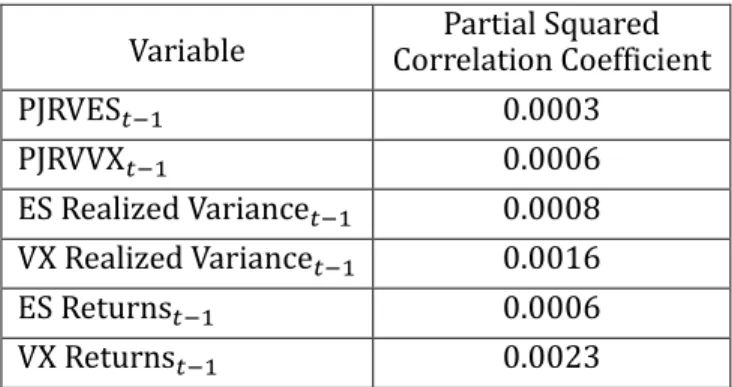
Table 8 Partial squared correlation coefficients As a control to this automated search
and as a way further to enquire into the role played byeach of the six variables in explaining the leverage effect, each of the candidate regressors was added to the initial baseline model (one at a time). The resulting estimates are reported in the Appendix. None of the added regressors ever manages to alter the sign or magnitude of the coefficients of the HAC-type regressors in a significant manner.
Also, none of the added regressors ever displays statistically significant coefficients. This stands as evidence that, despite the considerations listed above, lagged values of Realized Correlations still represent the primary explanatory variable of Realized Correlation itself. This impression is confirmed by the partial squared correlation coefficients40 computed after performing these last operations. The relatively small magnitude of these coefficients suggests that the individual contribution of each of the six variables to the explanatory power of the model is indeed limited.
40
A precise definition of the partial squared correlation and its interpretation has been provided by Agresti and Finaly (1999, p. 413). To compute these coefficients, each of the variables was added to the baseline HAR-type model, in turn.
Variable Correlation Coefficient Partial Squared
0.0003 0.0006 0.0008 0.0016 0.0006 0.0023
~ 21 ~
5. Insights Obtained and Final Remarks
This paper has investigated the dynamics of the leverage effect over time, using high frequency data. By applying Realized Kernel techniques, a more precise estimate of Realized Correlation – compared to standard subsampled estimators of Realized Correlation – was derived. This new measure avoids the so-called Epps effect and permits more clearly to observe the pattern in Realized Correlation. Regressing the resulting measure on a number of candidate explanatory variables, a deeper insight into the factors that determine the behavior of Realized Correlation over time (i.e., that influence the leverage effect) was obtained. In particular, volatility-related measures – and in particular the level of volatility-of-volatility – appears to dominate the actual level of the S&P 500 index in terms of explanatory power.
Acknowledgments:
I am much indebted to Dr. Kevin Sheppard for his helpful suggestions
on previous drafts of this work. The usual disclaimer applies.
References
[1] Agresti,A., and Finlay, B. (1999), Statistical Methods for the Social Science. Upper Saddle River NJ: Prentice Hall.
[2] Ait-Sahalia, Y., and Yu, J. (2008), “High Frequency Market Microstructure Noise Estimates and Liquidity Measures”, NBER Working Paper No. 13825: 1-40.
[3] Anderson, H.M., and Liao, Y. (2011), “Testing for Co-jumps with High-Frequency Financial Data: An Approach Based on First-High-Low-Last Prices”, Victoria, Australia: 7th International Symposium on Econometric Theory and Applications, April 2011 [Online] Available at:
https://editorialexpress.com/cgibin/conference/download.cgi?db_name=SETA2011 & paper_id=37
(June 19, 2011).
[4] Ates, A., and Wang, G.H.K. (2006), “Information Transmission in Electronic Versus Open-Outcry Trading Systems: An Analysis of U.S. Equity Index Futures Markets”, Journal of Futures Markets, 25(7): 679-715.
[5] Barndorff-Nielsen, O.E., Hansen, P.R., Lunde, A., and Shephard, N. (2008a), “Designing Realized Kernels to Measure the Ex-Post Variation of Equity Prices in the Presence of Noise”, Econometrica, 76(6): 1481-1536.
[6] Barndorff-Nielsen, O.E., Hansen, P.R., Lunde, A., and Shephard, N. (2008a), “Multivariate Realised Kernels: Consistent Positive Semi-Definite Estimators of the Covariation of Equity Prices with Noise and Non-Synchronous Trading. Oxford-Man Institute Working Paper, 1-42. [Online] Available: http://www.oxford-man.ox.ac.uk/~nshephard/papers/kernelMult_25_7_08. pdf (June 20, 2011).
[7] Barndorff-Nielsen, O.E., Hansen, P.R., Lunde, A., and Shephard, N. (2009), “Realized Kernels in Practice: Trades and Quotes”, Econometrics Journal, 12: C1-C32.
[8] Barndorff-Nielsen, O.E., and Shephard, N. (2004), “Power and Bipower Variation with Stochastic Volatility and Jumps”, Journal of Financial Econometrics, 2(1): 1-37.
[9] Black, F. (1976). “Studies of Stock Price Volatility Changes”, In: Alexandria VA (eds.), Proceedings of the American Statistical Association, Business and Economic Section: 177-181.
[10] Bollerslev, T., Litvinova, J., and Tauchen, G. (2006), “Leverage and volatility Feedback Effects in High Frequency Data”, Journal of Financial Econometrics, 4(3): 353-384.
[11] Bollerslev, T., Kretschmer, U., Pigorsch, C., and Tauchen, G. (2007), “A Discrete-Time Model for Daily S&P 500 Returns and Realized Variations: Jumps and Leverage Effects”, Journal of Econometrics, 150(2): 151-166.
[12] Bollerslev, T., Tauchen, G., and Zhou, H. (2009), “Expected Stock Returns and Variance Risk Premia”, Review of Financial Studies, 22(11): 4463-4492.
[13] Bouchaud, J., Matacz, A., and Potters, M. (2001), “The Leverage Effect in Financial Markets: Retarded Volatility and Market Panic”, Physical Review Letters, 87(22): 1-4.
Review of Economics & Finance
~ 22 ~
[14] CBOE (2007), “CFE Information Circular IC07-03: Rescaling of VIX and VXD Futures Contracts”, Chicago Board Options Exchange, March 7. [Online] Available at: http://cfe.cboe.com/framed/ PDFframed.aspx?content=/publish/CFEinfocirc/CFEIC07-003%20.pdf§ionName=SECAB OUTCFE&title=CBOE%20-%20CFEIC07-003%20Rescaling%20of%20VIX%20and%20VXD%
20 Futures%20Contracts (June 9, 2011).
[15] CBOE (2011), “Products Specifications”, Chicago Board Options Exchange, [Online] Available at:
http://www.cfe.cboe.com/Products/Spec_VIX.aspx (June 9, 2011).
[16] CBOE, (2003), “VIX: CBOE Volatility Index”, Chicago Board Options Exchange, [Online] Available at: http://www.cboe.com/micro/vix/vixwhite.pdf (June 9, 2011).
[17] Chan, K., Chockalingam, M., and Lai, KWL. (2000), “Overnight Information and Intraday Trading Behavior: Evidence from NYSE Cross-Listed Stocks and Their Local Market Information”, Journal of Multinational Financial Management, 10: 495-509.
[18] Cheung, Y.W., and Ng, L. (1992), “Stock Price Dynamics and Firm Size: An Empirical Investigation”, Journal of Finance, 47(5): 1985-1997.
[19] Christie, A. (1982), “The Stochastic Behavior of Common Stock Variances: Value, Leverage, and Interest Rate Effects”, Journal of Financial Economics, 10(4): 407-432.
[20] Chung, H., and Chiang, S. (2006), “Price Clustering in E-mini and Floor-traded Index futures”, Journal of Futures Markets, 26(3): 269-295.
[21] CME Group (2011), “S&P 500 Futures and Options”, Chicago Mercantile Exchange, [Online] Available at: http://www.cmegroup.com/trading/equity-index/files/SxP500_FC.pdf (June 9, 2011). [22] Corsi, F.(2009), “A Simple Approximate Long-Memory Model of Realized Volatility”, Journal of
Financial Econometrics, 7(2): 174-196.
[23] De Pooter, M., Martens, M., and Van Dijk, D. (2006), “Predicting the Daily Covariance Matrix for S&P 100 Stocks Using Intraday Data - But Which Frequency to Use?” Tinbergen Institute Discussion Papers, No. 2005-089/4: 1-34.
[24] Dickey, D.A., and Fuller, W.A. (1979), “Distribution of the Estimators for Autoregressive Time Series with a Unit Root”, Journal of the American Statistical Association, 74(366): 427-431.
[25] Domowitz, I., and Steil, B. (1999), “Automation, Trading Costs and the Structures of the Securities Trading Industry”, In: R.E. Litan, and A.M. Santomero (Eds.), Brookings-Wharton Papers on Financial Services, Washington DC: Brookings Institution Press (1999): 33-92.
[26] Duffee, G. (1995), “Stock Returns and Volatility: A Firm Level Analysis”, Journal of Financial Economics, 37(3): 399-420.
[27] Epps, T.W. (1979), “Comovements in Stock Prices in the Very Short Run”, Journal of the American Statistical Association, 74(366): 291-298.
[28] Figlewski, S., and Wang, X. (2000) “Is the “Leverage Effect” a Leverage Effect?” Technical Report, NYU Stern School of Business and City University of Hong Kong, [Online] Available:
http://papers.ssrn.com/sol3/papers.cfm?abstract_id=256109 (16 May 2011)
[29] French, K.R., Schwert, G.W., and Stambaugh, R.F. (1987), “Expected Stock Returns and Volatility”, Journal of Financial Economics, 19: 3-29.
[30] Gatheral, J., and Oomen, R.C.A. (2010), “Zero-Intelligence Realized Variance Estimation”, Finance and Stochastics, 14(2): 249-283.
[31] Giot, P. (2002), “Implied Volatility Indices as Leading Indicators of Stock Index Returns?” CORE Discussion Paper, No. 2002/50: 1-29.
[32] Glosten, L.R., Jaganathan, R., and Runkle, D.E. (1993), “On the Relation Between the Expected Value and the Volatility of the Nominal Excess Returns on Stocks”, Journal of Finance, 48(5): 1779-1801.
[33] Hasanhodzic, J., and Lo, A.W. (2011), “Black’s Leverage Effect is not due to Leverage”, Working Paper, [Online] Available: http://papers.ssrn.com/sol3/papers.cfm?abstract_id= 1762363 (16 May 2011).
~ 23 ~
[34] Hasbrouck, J. (2003), “Intraday Price Formation in U.S. Equity Index Markets”, Journal of Finance, 58(6): 2375-2400.
[35] Keim, D.B. (1983), “Size-Related Anomalies and Stock Return Seasonality: Further Empirical Evidence”, Journal of Financial Economics, 12(1): 13-32.
[36] Lu, Z., and Zhu, Y. (2009), “Volatility Components: The Term Structure Dynamics of VIX Futures”, Journal of Futures Markets, 30(3): 230-256.
[37] Manda, K. (2010), “Stock Market Volatility during the 2008 Financial Crisis”, Working Paper, Glucksman Institute for Research in Securities Markets: 1-32.
[38] Martens, M. (2002), “Measuring and Forecasting S&P 500 Index-Futures Volatility Using High-frequency Data”, Journal of Futures Markets, 22(6): 497-518.
[39] Moosa, I.A., and Bollen, B. (2001), “Is There a Maturity Effect in the Price of the S&P 500 Futures Contract?” Applied Economic Letters, 8(11): 693-695.
[40] Muranaga, J., and Shimizu, T. (1999), “Market Microstructure and Market Liquidity”, IMES Discussion Paper Series, 99-E-14: 1-17.
[41] Nelson, D.B. (1991), “Conditional Heteroskedasticity in Asset Returns: A New Approach”, Econometrica, 59(2): 347-370.
[42] Schroeder, L.D., Sjoquist, D.L., and Stephan, P.E. (1986), Understanding Regression Analysis: An Introductory Guide. Newbury Park CA: Sage University Paper Series on Quantitative Applications in the Social Sciences.
[43] Simon, D.P. (2003), “The NASDAQ Volatility Index During and After the Bubble”, Journal of Derivatives, 11(2): 9-24.
[44] Simon, D.P., and Wiggins, R.A. (2001), “S&P Futures Returns and Contrary Sentiment Indicators”, Journal of Futures Markets, 21(5): 447-462.
[45] Sun, Y., and Wu, X. (2010), “A Nonparametric Study of Dependence Between S&P 500 Index and Market Volatility Index(VIX)”, Beijing: European Financial Management Symposium on Asian Finance, April: 1-21.
[46] Szado, E. (2009), “VIX Futures and Options: A Case Study of Portfolio Diversification During the 2008 Financial Crisis”, Journal of Alternative Investment, 12(2): 68-85.
[47] Whaley, R.E. (1993), “Derivatives on Market Volatility: Hedging Tools Long Overdue”, Journal of Derivatives, 1(1): 71-84.
[48] Whaley, R.E. (2000), “The Investor Fear Gauge”, Journal of Portfolio Management, 26(3): 12-17. [49] Wood, R.A., McInish, T.H., and Ord, J.K. (1985), “An Investigation of Transaction Data for NYSE
Stocks”, Journal of Finance, 40(3): 723-741.
Appendix: Adding Individual Variables to the Baseline Model
(1) Percentage of Jumps in the Realized Variance of ES contracts
Regression results – Predicting Realized Correlation
-0.0235 (0.0279) 0.1074 (0.1044) 0.0382 (0.0624) 0.7362 (0.1040) *** 894 -0.3441 0.2282 -0.3173 0.2247 -0.3339 0.8396 302.6572 -1134.8619 0.0000
(2) Percentage of Jumps in the Realized Variance of VX contracts
Regression results – Predicting Realized Correlation
Review of Economics & Finance
~ 24 ~ 0.0381 (0.0534) 0.7348 (0.1042) *** 894 -0.3449 0.2288 -0.3181 0.2254 -0.3347 0.8393 294.8523 -1134.6118 0.0000(3) Realized Variance of ES contracts
Regression results – Predicting Realized Correlation
0.0152 (0.0302) 0.1094 (0.1082) 0.0388 (0.0553) 0.7311 (0.1018) *** 894 -0.3436 0.2279 -0.3168 0.2244 -0.3334 0.8398 294.8035 -1135.0087 0.0000
(4) Realized Variance of VX contracts
Regression results – Predicting Realized Correlation
0.0197 (0.0260) 0.1088 (0.1162) 0.0389 (0.0598) 0.7341 (0.1072) *** 894 -0.3439 0.2280 -0.3171 0.2246 -0.3336 0.8397 285.8783 -1134.9368 0.0000 (5) Returns on ES contracts
Regression results – Predicting Realized Correlation
0.0212 (0.0357) 0.1100 (0.1111) 0.0357 (0.0522) 0.7367 (0.1045) *** 894 -0.3440 0.2281 -0.3171 0.2246 -0.3337 0.8397 284.1397 -1134.9113 0.0000 (6) Returns on VX contracts
Regression results – Predicting Realized Correlation
-0.0407 (0.0265) 0.1115 (0.1027) 0.0313 (0.0424) 0.7395 (0.1024) *** 894 -0.3456 0.2294 -0.3188 0.2259 -0.3353 0.8390 322.5568 -1134.3976 0.0000
Notes: 1. Six tables above report regression coefficients followed by standard errors in parentheses. 2. *, **, *** indicate statistical significance at the 10%, 5% and 1% levels, respectively. 3. The model includes an intercept which is not reported.