A Description of the Madden–Julian Oscillation Based on a Self-Organizing Map
RAJIBCHATTOPADHYAY
Indian Institute of Tropical Meteorology, Pune, India
AUGUSTINVINTZILEOS
University of Maryland, College Park–ESSIC, and Climate Prediction Center, NOAA/NWS/NCEP, College Park, Maryland
CHIDONGZHANG
Rosenstiel School of Marine and Atmospheric Sciences, University of Miami, Miami, Florida
(Manuscript received 19 February 2012, in final form 27 July 2012) ABSTRACT
This study introduces a nonlinear clustering technique based on a self-organizing map (SOM) algorithm to identify horizontal and vertical structures of the Madden–Julian oscillation (MJO) through its life cycle. The SOM description of the MJO does not need intraseasonal bandpass filtering or selection of leading modes. MJO phases are defined by SOM based on state similarities in chosen variables. Spatial patterns of rainfall-related variables in a given MJO phase defined by SOM are distinct from those in other phases. The structural evolution of the MJO derived from SOM agrees with those from other methods in certain aspects and differs in others. SOM reveals that the dominant longitudinal structure in the diabatic heating and related fields of the MJO is a dipole or tripole pattern with a zonal scale close to that of zonal wavenumber 2, as opposed to zonal wavenumber 1 suggested by other methods. Results from SOM suggest that the MJO life cycle may be composed of quasi-stationary stages of strong, coherent spatial patterns with relatively fast transition in between that is less coherent and weaker. The utility of SOM to isolate signals of an individual MJO event in a case study is illustrated. The results from this study show that some known gross features of the MJO are independent of diagnostic methods, but other properties of the MJO may be sensitive to the choice of di-agnosis method.
1. Introduction
Many methods have been used to isolate signals of the Madden–Julian oscillation (MJO; Madden and Julian 1972, 1994) from other subseasonal perturbations. Commonly used methods can be broadly classified as based on correlation or regression (Rui and Wang 1990), empirical orthogonal function (EOF; Lau and Chan 1986; Knutson and Weickmann 1987; Zhang and Hendon 1997; Wheeler and Hendon 2004; Weare 2003; Maloney and Shaman 2008), and power spectrum (Salby and Hendon 1994; Wheeler and Kiladis 1999; Roundy and Schreck 2009). Each of them bears advantages and
limitations. Applications to MJO diagnostics based on EOF and principal components (PCs) have been rec-ommended as standard metrics for the study of the MJO (Waliser et al. 2009). To a certain degree, our perception of the MJO, especially its spatiotemporal characteris-tics, is from results derived using EOF-based methods. Among different version of EOF methods, the real-time multivariate MJO (RMM) index (Wheeler and Hendon 2004) has been commonly used in many applications because it provides a simple and common way of making and comparing composites of different variables through the life cycle of the MJO as depicted by its eight phases. While the utility of this index is undeniable, its limitation has been noticed. The readily available RMM index time series is not subject to intraseasonal bandpass fil-tering for good reasons (Wheeler and Hendon 2004) but, because of this, it includes signals not belonging to the MJO, which can be dominant at times (Roundy and
Corresponding author address: Rajib Chattopadhyay, CGM Division, Indian Institute of Tropical Meteorology, Dr. Homi Bhabha Road, Pune-411008, India.
E-mail: [email protected] DOI: 10.1175/JCLI-D-12-00123.1 Ó2013 American Meteorological Society
Schreck 2009; Roundy et al. 2009). The widely used eight phases of the MJO defined by the RMM index or any PC-based time series (viz., dividing 3608 equally into eight sections of 458on the phase diagram composed of the two leading PCs) are arbitrary for convenience (Zhang and Hagos 2009). There are infinite numbers of ways to define eight phases of 458that are equally valid. A composite of any variable propagating with the MJO in a given phase is an average not only over different events but also over a period of time within a single event; thus, certain signals in spatial structures might be lost (Zhang and Ling 2012). In this study, we introduce an application of a clus-tering method based on a self-organizing map (SOM; Kohenen 1990) to identify MJO phases to compare with those based on the RMM index. The main purpose is to see how much of what we know about the MJO structure and evolution from using the RMM index can be re-produced by a completely different method (SOM) and what SOM may produce that we have not seen by using the RMM index. The similarities between results from the two methods would enhance our confidence to our existing knowledge about the MJO. Their discrepancies may bring new challenges to the MJO study and en-courage us to explore more.
The SOM technique is frequently used to extract time evolution of a wide variety of geophysical events or episodes, such as extreme weather events (Cavazos 1999; Hewitson and Crane 2002), El Nin˜o (Leloup et al. 2007), monsoon intraseasonal oscillation (Chattopadhyay et al. 2008), Indian Ocean dipole (Iskandar et al. 2008; Tozuka et al. 2008), and ocean current variability (Liu and Weisberg 2005; Liu et al. 2006). It has the following unique characteristics:
(i) It does not depend on any fixed reference point as in the regression method.
(ii) It does not require orthogonality, as does the EOF method, that may not be physical.
(iii) It does not rely on leading mode selection (EOF) or filtering (spectrum) that includes only a fraction of information in a dataset.
(iv) It can be applied to a short data record for case studies, and it does not suffer from data gaps, as does a Fourier transform method.
Data and SOM methodology are introduced in section 2 with technical details described in the appendices. Horizontal structures and evolution of the MJO based on SOM and the RMM index applied to the same data are compared in section 3. Vertical structures of the MJO extracted by SOM and the RMM index are com-pared in section 4. The utility of SOM in case studies is demonstrated in section 5. Section 6 provides a summary and concluding remarks.
2. Data and method
a. Data
Data used in this study include daily National Oceanic and Atmospheric Administration (NOAA) outgoing longwave radiation (OLR) from 1979 to 2008 (Liebmann and Smith 1996) and winds, temperature, and humidity from Modern Era Retrospective Analysis (MERRA) data for 1997–2009 (Rienecker et al. 2011). Heating sources (Q1) and moisture sinks (Q2) were estimated from the MERRA reanalysis data following the method of Yanai et al. (1973).
Only data in November–April were used in the di-agnostics of the boreal winter/spring MJO that shows predominantly eastward propagation as opposed to the boreal summer MJO that exhibits both eastward and northward propagation (Lawrence and Webster 2002). For a given field, its daily anomalous time series was generated by removing its daily climatology (av-erages of all same calendar days). In the case of Q1, its anomalies were normalized by its daily standard deviation at each vertical level before SOM was ap-plied. This allows weaker but physically important Q1 at lower and upper levels to equally contribute to the SOM analysis. Finally, any residual November–April mean was removed. Composites were made, however, with unnormalized anomalies. No intraseasonal band-pass filtering was applied to any of the data at any analysis stage.
b. Method
The SOM is a clustering algorithm that can identify dominant patterns in a dataset (Kohenen 1997; Liu et al. 2006). Here, SOM is used to identify a sequence of spatial patterns that distinguish from each other and may represent structural evolution of a phenomenon. When applied to the MJO, an important difference be-tween SOM and the RMM index is that, once the number of phases desired (N) is determined, the distinct spatial patterns that may defined MJO phases (i.e., zonal locations of its convection center) given by SOM are unique. The SOM technique is also more effective to extract distinct patterns when there are nonlinear manifolds, stochastic noise (low signal to noise ratio), or gaps in the data (de Bodt et al. 1997; Cottrell and Letre´my 2007; Liu et al. 2006). SOM identifies spatial patterns by grouping similar subset of the input data into clusters, also known as nodes.
Given a dataset ofm3n3Tdimension, wheremcan be longitude,ncan be latitude or vertical level, andTis total time points, we search for N (N T) distinct patterns (i.e., nodes) ofm3ndimension. A given pat-tern (node)Sj(j51, 2,. . .,N) is composed of the data at
a number of time points (a subset ofT,Tj 4T) that share a similarity, while any two patterns are distinctly different from each other based on an objective crite-rion. OnceNnodes are determined by SOM, any vari-ables can be averaged for a given node (i.e., over time
Tj). This average is equivalent to a composite, which is of no difference from other composite techniques. In the case of the MJO, the sequential order of theNpatterns should represent the structural evolution through its life cycle, similar to the sequential order of the phases de-fined by the RMM index. Similar to the other methods, there is no objective or standard way to determine the optimal number of nodes (patterns) N that can best represent a given dataset. Often, physical arguments or other decision tools (e.g., hierarchical clustering, linear vector quantizer) are invoked (Kohenen 1997). We recommend an estimated range ofNfor the MJO study in appendix A. The technical details to implement SOM are discussed in appendix B. To further test the utility of SOM, it was applied to a dataset of a pure space–time sinusoidal wave. SOM is able to extract the sinusoidal signal with a specific order of time sequence in ampli-tude and position (not shown). When SOM was applied to white noise in space and time, it gave random patterns without any dominant time sequence.
In this study, SOM was applied to data of two dimen-sions in longitude (m5144; 08–3608) and latitude (n514; 158S–158N) at a given vertical level or in longitude (m5
144) and vertical levels (n525; 1000–200 hPa) with an average in latitude between 158S and 158N. The study period covers November–April of 12 consecutive years, 1997–2009 (T518231252184 days). Each day was assigned to a node by SOM. Composites for each node were plotted for a given anomalous time series. The statistical significance of a composited pattern for a node is estimated using the Student’sttest against a null hy-pothesis that the composited anomalies are not different from zero. Using appendix A, nine nodes (N59) were used to extract MJO signals for the purpose of com-paring to the eight RMM phases with one node dis-carded (explained below). The eastward-propagating signals that represent the MJO can be extracted by SOM using a wide range ofN.
Once SOM clustering is completed, each node is con-nected to the others through a time sequence of evolu-tion. At a given timetnodeSj,tmay be followed at time
t11 by the same nodeSj,t11or a different nodeSk,t11.
If most of the time Sj1,tis followed bySj2,t11, then the
sequence from nodesSj1toSj2may represent an optimal
structural evolution in the data. An example of such optimal structural evolution is demonstrated in Fig. 1a, which shows the probability of the time sequence be-tween 3 3 3 SOM nodes derived from daily OLR
anomalies as input. The probability is measured by the length of arrows pointing to the direction from one node to another. For each node, the longest arrow represents the most probable direction of the structural evolution. Transitions are possible from a given node to any other node. However, the most probable sequence moves clockwise through the peripheral nodes in this figure. Node (2, 2) does not have any preferable sequence and does not represent any systematic structural evolution of the data. It will not be included as part of the struc-tural evolution. This arrow plot is unique for each SOM analysis. When SOM was applied to a synthetic data composed of same OLR anomalies but with the time sequence randomly rearranged, identical clustered no-des were found as for the original OLR anomalies but its arrow plot does not show any preferable time sequence. Figure 1b shows the histogram of the number of suc-cessive input days that remain on the same nodes. Such successive days may suggest the time scale of a node. Some nodes [e.g., (1, 1), (1, 3), (3, 3) and (3, 1)] shows more occurrence of longer time scales ($7–9 days) than the others. The contributions from a wide range of time scales to these nodes may suggest the multiscale nature of the MJO (Nakajawa 1988; Majda and Biello 2004), especially the existence of high-frequency (2–3 days) events (Shibagaki et al. 2006; Kikuchi and Wang 2010). The possible meaning of the uneven distribution of days among the nodes will be further discussed in section 4.
3. Horizontal structures
Composites of daily anomalies in OLR and 850-hPa wind vectors for the peripheral nodes in Fig. 1a are shown in Fig. 2 (left). The nodes are arranged in the sequence of (1, 3)/(2, 3)/(3, 3)/(3, 2)/(3, 1)/(2, 1)
/(1, 1)/(1, 2) according to the most probable sequence direction (longest arrows) shown in Fig. 1a. There is a clear signal of eastward propagation of the OLR anomaly centers and their associated anomalies in the wind field from the Indian Ocean to the central Pacific through the eight nodes. Node (1, 3) was chosen as node 1 because it may represent a phase immediately prior to a convective onset (negative OLR anomalies) over the tropical Indian Ocean in the next node (2, 3) or node 2. This convection center is strengthened in node 3 and moves eastward continuously afterward. It passes over the Maritime Continent in nodes 5–7 and become much weaker over the western Pacific in nodes 8, 1, and 2. The decay of the convection center over the central Pacific and the initiation of a new convection center over the Indian Ocean occur simultaneously in nodes 2 and 3.
This cyclical sequence of the structural evolution in clustered OLR anomalies is very similar to the known
canonical pattern of MJO propagation (Madden and Julian 1994; Hendon and Salby 1994; Wheeler and Hendon 2004). The MJO evolution based on the eight phases defined by the RMM index (Wheeler and Hendon 2004) for the same period (1979–2009) is shown in the right column of Fig. 2. Even though there is no obvious one to one match between the SOM nodes and RMM phases, the similarities in the structural evolutions of OLR and wind based on the completely different two methods are striking. These similarities demonstrate the utility of SOM in extracting the known MJO signals. They also confirm that robust signals in the large-scale distributions of convection and winds through the life cycle of the MJO are independent of the analysis methods.
Because there was no time filtering applied to the OLR data as input to the SOM analysis, the structural evolution in Fig. 2 does not include explicit information
of time scales. Its representation of the MJO needs to be further confirmed by the spectral behavior of the clustered patterns. A space–time spectrum of the SOM clustered patterns can be calculated using a reconstructed time series including only the eight patterns shown in the left column of Fig. 2 (explained at the end of appendix B). Following the method of Wheeler and Kiladis (1999), the equatorial symmetric space–time spectrum of the reconstructed SOM series is plotted in Fig. 3a, along with the spectrum of the original anomalous daily OLR (Fig. 3b). Both clearly show a spectral peak at 20–80 days and eastward-propagating zonal wavenumbers 1–3. Meanwhile, it is clear that the SOM spectrum does not have obvious signals that may suggest the existence of the equatorial Kelvin and Rossby waves as in the spec-trum of original OLR anomalies. In this sense, MJO signals come out as the dominant pattern of the daily OLR anomalies from the SOM clustering process FIG. 1. (a) Direction of transition between each node. (b) Distribution of events that last greater than or equal to two consecutive days in
each node.
FIG. 2. (left) Composites of eight SOM nodes of OLR anomalies (colors; W m22) and wind vectors (m s21) for November–April of 1979–2008. OLR is plotted only when its amplitude is above the 95% significance level. Wind vectors with amplitudes above the 95% significance level are plotted as thick arrows. (right) As in (left), but for RMM phase composites.
without any spectral filtering. The ratio of eastward and westward power for a time period between 30 and 90 days and wavenumbers between61 to65 is 2.86 in the SOM spectrum, while it is 1.83 in the spectrum of the original daily OLR. This further demonstrates the ability of SOM clustering to identify the eastward-moving MJO signal. To further highlight the MJO spec-tral power, we followed Wheeler and Kiladis (1999) to remove the red background from the SOM spectrum (Fig. 3c) and the original OLR spectrum (Fig. 3d). The spectrum above red background is comparable to the Markov clustering spectrum (Fig. 16 of Jones 2009). However, there are some very-high-frequency compo-nents in the SOM spectrum. This may be the artifact of clustering since every day has to be clustered in any of
the nine nodes. This discretization can introduce addi-tional noise frequencies in clustered sample (Widrow and Kolla´r 2008). The spectral peak at zonal wave-number 2 and intraseasonal time scale, representing the MJO, stands out unambiguously. The isolation of the MJO spectral signal was done by SOM without any applications of bandpass filtering (as by Fourier trans-form) or selection of leading modes (as by EOF). Other equatorial perturbations (e.g., the Kelvin wave) that may contaminate the MJO signals derived by the RMM index (Roundy et al. 2009) are absent. The MJO spectral peak seen in Figs. 3a,c completely disappears when the SOM analysis is applied to a time series of 1-hPa tem-perature from MERRA or a reconstructed OLR time series consisting of the eight node patterns shown in FIG. 3. Space–time spectra of reconstructed OLR using (left) SOM composites and (right) original OLR. (top) The
total spectra and (bottom) spectral power above the red noise background.
Fig. 2 randomly resampled in longitude. No MJO signal is expected in either case.
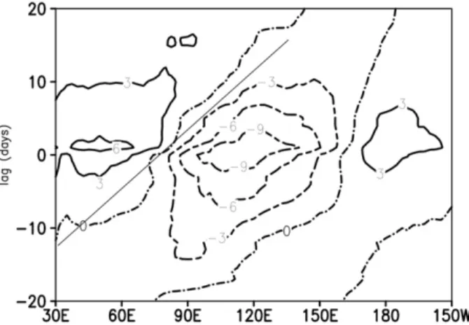
The eastward propagation phase speed of the clus-tered patterns can be estimated through a lag com-posite of the same reconstructed time series of OLR including only the eight node patterns shown in the left column of Fig. 2 as for constructing the spectrum. Node 5 was chosen as a reference point (lag 0). The overall eastward phase propagation speed demonstrated in this lag composite (Fig. 4) is slightly less than 5 m s21 (marked by the straight line). There are obvious sta-tionary signals.
Notwithstanding the similarity between the com-posites of OLR anomalies using the SOM and RMM index, there are discrepancies that should also be no-ticed. The peaks of OLR anomalies (both positive and negative) in the SOM composites (Fig. 2, left) appear to be larger than in the RMM composites (Fig. 2, right), especially over the western Pacific. The SOM composites exhibit a ‘‘tripole’’ structure with a main peak flanked by two minor peaks of the opposite sign on both western and eastern sides (e.g., nodes 2 and 7). This tripole structure is much weaker in the RMM composites (e.g., phases 1, 5, and 6). Differences be-tween the MJO signals extracted by the two methods are more obvious in the vertical–longitude cross sec-tion along the equator, which are shown in the next section.
4. Vertical structures
Following the same procedure as for the OLR anomalies in section 3, we applied SOM to Q1 anom-alies averaged over 158S–158N (dimension ofm5144
longitude,n525 vertical levels) with nine nodes, se-lected eight nodes, and determined their sequential order to represent the dominant structural evolution. Node 1 was chosen for the same reason as for the OLR nodes in Fig. 2. Composites for each node were made for Q1, temperatureT, and zonal and vertical wind vectors (Fig. 5, left). Only results with the confidence level equal or above 95% were plotted (Q1 and wind vectors) or highlighted (temperature contours). Composites of the same fields based on the eight RMM phases are also shown in Fig. 5 (right) for comparison. The eastward propagation of heating/cooling maxima from the Indian to western Pacific Oceans (Zhang et al. 2010) is evident in both SOM and RMM composites. Both show the vertical structure in temperature anomalies with an east-ward and upeast-ward tilt above the 200-hPa level. Both show robust vertical overturning circulations connecting the heating–cooling dipoles (Sperber 2003).
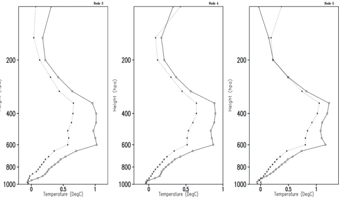
There are, however, more obvious discrepancies be-tween the two composites in Fig. 5 than those for OLR in Fig. 2. There is a sign of westward tilt in Q1 (Lin et al. 2004; Kiladis et al. 2005) and vertical motions (Sperber 2003) in certain RMM phases (e.g., 3, 4, 7, and 8) in Fig. 5. Such a westward tilt structure is not obvious at all in the SOM Q1 composites. Q1 anomalies in the SOM composites are stronger than in the RMM composites. So are the temperature anomalies. Particularly, positive Q1 anomalies (heating) in the SOM composite (Fig. 5, left) appear to have larger amplitude below the freezing levels (;500 hPa) than those in the RMM composites (Fig. 5, right). This is more obvious in Fig. 6, where area-averaged vertical profiles of Q1 for nodes/phases 3–5 are plotted. While Q1 maxima in both SOM and RMM tend to spread vertically across the freezing level between 300 and 600 hPa, there is a second lower peak near 600 hPa in SOM Q1 that is absent in RMM Q1. In neither com-posite are low-level heating peaks near 700 hPa visible, as seen in other EOF-based diagnostics of MJO heating (Hagos et al. 2010; Ling and Zhang 2010). While zonal heating–cooling dipoles (Lau and Phillips 1986) exist in both SOM and RMM composites, RMM Q1 tends to show a monopole structure more often (phases 1, 3, 4, and 8) than in the SOM composites. The monopole structure in Q1 and its associated circulations in the RMM composite lead to a perception that the zonal scale of the MJO is that of zonal wavenumber 1. The zonal scale of the dipole structure in SOM with the heating and cooling peaks next to each other is of zonal wavenumber 2 (the zonal wavelength, measured by the double distance between the heating and cooling cen-ters, is about 1608).
We now examine these differences in more details. For each RMM phase, there are sets of days that are also FIG. 4. Latitudinally (158S–158N) averaged lag composite using
the reconstructed OLR time series of SOM composite. Node 5 in Fig. 2 is the reference point (lag 0). The straight line shows 5 m s21 phase speed. Amplitudes are unitless.
FIG. 5. (left) Pressure–longitude composite of anomalies in diabatic heating (Q1; colors; K day21), wind vectors (m s21),
and temperature (T; contours with interval 0.28C without 0 contours) for SOM nodes. (right) As in (left), but for RMM phases. Results of 95% significance are plotted for Q1 and highlighted as thick contours forTand thick vectors for winds.
in a given SOM node. LetRidenote an RMM phase,Sj denote a SOM node,n(Ri) denote the total days inRi,n
(Sj) denote the total days inSj,n(Ri \ Sj) denote the common days inRiandSj,n(ORij)5n(Ri)2n(Ri\Sj) denote the days inRibut not inSj, andn(OSji)5n(Sj)2
n(Ri\Sj) denote the days inSjbut not inRi. Figure 7a illustrates overlapping and nonoverlapping days be-tween Ri and Sj. Figure 7b shows the distribution of overlapping days for eight RMM phases and eight SOM nodes derived from Q1. Bold numbers indicate the RMM phase that shares the largest number of common days with a given SOM node. Underlined numbers in-dicate the SOM node that shares the largest number of common days with a given RMM phase. An optimum match between SOM nodes and RMM phases would lead to the largest number in any row or column in the diagonal elementsn(Ri\Sj). To an extreme, zero non-diagonal elements would imply that SOM and RMM patterns are identical. The similarities between the re-sults from the two methods are indicated by the large numbers along the diagonal for certain SOM nodes and RMM phases, such asn(R3\S3),n(R5\S5), and
n(R7\S7). However, RMM phases 6 and 4, for example,
also share significant numbers of days with SOM node 5. Out of total 309 days in RMM phase 5, 130 days share the same spatial pattern as suggested by SOM node 5
and others do not. SOM node 1 matches the best RMM phase 2 instead of phase 1. There are RMM phases (e.g., 1 and 4) that do not have a single dominant spatial pattern in Q1 that would be suggested by a number of overlapping days with a SOM node much greater than other SOM nodes. Some spatial patterns represented by SOM nodes (e.g., 2, 4, 6, 8) cannot be represented by any single RMM phase. When the distribution diagram is based on a different variable (e.g., OLR) or days with amplitudes of the RMM index equal to or greater than one, a measure of strong MJO events (Wheeler and Hendon 2004), the result remains qualitatively the same.
It is noticed that days are more evenly distributed among the RMM phases than SOM nodes. Also, there appears to be more days in the odd than even SOM nodes. We have seen from Fig. 1b that the odd SOM nodes include more consecutive days than the even nodes. Figure 2 indicates that OLR anomalies are stronger in the odd than even SOM nodes. The largest overlapping days between SOM nodes and RMM phases all occur in the odd SOM nodes (Fig. 7b). The exact meaning of such peculiar behaviors of the SOM nodes is not im-mediately clear. It may suggest that the evolution of large-scale convection of the MJO undergoes several quasi-stationary stages that are well organized with large FIG. 6. Area-averaged vertical profile over the region of maximum heating for node (phase) 3, 4, and 5. All the panels are latitude averaged between 158S and 158N. The longitudinal extent for averaging node (phase) 3, 4, and 5 are 1008–1208E (908–1008E), 1108–1308E (1008–1108E), and 1408–1608E (1208–1308E). Solid curves are for SOM, and dotted curves are for RMM.
anomalies. In between are transition stages that are less well organized with smaller anomalies and relatively fast eastward movement. If so, such uneven evolution of MJO convection is not captured by the RMM phases.
The few large numbers on the diagonal in Fig. 7b, a sign of the consistency between MJO signals derived from the SOM and RMM methods, indicate that more than 50% of SOM node and RMM phases are not overlapping. The nonoverlapping days spread throughout all other nodes and phases but more in the neighboring nodes and phases. This suggests that a given RMM phase may represent a dominant but not unique spatial structure of Q1 defined by SOM. No unique spatial structure of Q1 defined by SOM can be represented solely by any single RMM phase.
To gain further insight into the discrepancies between the two methods, we made composites based on their overlapping days,n(Ri\Si) along the diagonal of Fig. 7b, and nonoverlapping days,n(OSii,) andn(ORii) for Q1,
T, and winds (Fig. 8). The eastward propagation of Q1
anomalies is evident in all three composites. However, the discrepancies among the three are more visible and intriguing. Days n(OSii) and n(Ri \ Si) belong to the same SOM node i, so the patterns in their composites (Fig. 8, left and middle) are expected to be the same. They are whenn(Ri\Si) is large (e.g.,i55). Otherwise, they are different mainly because insignificant results are not plotted.1Days of n(OSii) and n(ORii) are dif-ferent, so should their composites. The Q1 dipole pat-tern is evident in then(OSii) composites (Fig. 8, left) but not in the n(ORii) composites, which obviously miss cooling signals in many phases (Fig. 8, right).
The top-heavy Q1 structure seen in Fig. 5 is a unique results of the RMM composites. It does not appear in the
n(Ri\Si) composites (Fig. 8, middle). The monopole structure seen in the RMM composites (Figs. 2, 5) be-come even more obvious in then(ORii). Meanwhile, the dipole structure in the SOM Q1 composites is preserved in n(OSii). This might be the most distinct difference between the results based on the SOM and RMM methods. Implications of this and other differences between the two methods will be further discussed in section 6.
The moisture-related thermodynamical structures of the MJO [viz., composites of moisture sinks (Q2), spe-cific humidity (q), and zonal/vertical wind vectors] are shown in Fig. 9 for the same SOM nodes as in Fig. 5. Maximum moisture sinks (positive anomalies in Q2) are located at the same longitudes as maximum heating (positive anomalies of Q1; Fig. 5). Positive and negative Q2 anomalies appear side by side in most nodes (except node 8), giving a dipole structure as in Q1. The double-peak vertical structure in Q2 (Yanai and Tomita 1998; Thayer-Calder and Randall 2009) is clearly seen at most nodes, with the primary peak located between 500 and 400 hPa and the secondary peak near 700 hPa. The two peaks are mostly in phase. Strongest anomalies in spe-cific humidityqare in the lower troposphere, with their maxima near 700–600-hPa levels (Sperber 2003), almost overlapping with Q2 maximum anomalies. Low-level (below the 700-hPa level)qanomalies east of midlevel peaks are seen over the Indian Ocean and Maritime Continent (nodes 1–5) but not over the western Pacific. This low-level moistening prior to or east of the deep convection center of the MJO has been documented previously (e.g., Jones and Weare 1996; Myers and Waliser 2003; Tian et al. 2010; Benedict and Randall 2007; Kiladis et al. 2005) and has motivated thoughts that place interaction between convection and environmental FIG. 7. (a) Schematic diagram illustrating overlapping and
non-overlapping days between SOM nodes and RMM phases. (b) Distributions of overlapping days between SOM node and RMM phase. Underlined numbers indicate the SOM node that shares the most days with a given RMM phase. Bold numbers indicate the RMM phase that shares the most days with a given SOM node. The total number of days of each RMM phase is given at the right of each row and the total number of days for each SOM node is given at top of each column.
1Significance varies with the number of days shared by the
corresponding RMM phase inn(Rj\Si).
FIG. 8. As in Fig. 5, but for composites of (left) the SOM nodes using days not overlapping with their corresponding RMM phasesn(OSji), (middle) days that are shared by corresponding SOM nodes and RMM phasesn(Ri\Si), and (right) RMM phases using days not overlapping with their corresponding SOM nodesn(ORii).
humidity at the center of MJO dynamics (Raymond and Fuchs 2009; Thayer-Calder and Randall 2009; Hannah and Maloney 2011).
5. Case study
We now demonstrate how SOM can be applied to case studies for individual MJO events with short data records. As an example, we take the MJO events during the Tropical Ocean and Global Atmosphere Coupled Ocean–Atmosphere Response Experiment (TOGA
COARE; Webster and Lukas 1993) period (November 1992–February 1993), which were described by Yanai et al. (2000). The RMM index (Wheeler and Hendon 2004) suggests that the event of January–February 1993 was a strong one (with the standardized RMM index greater than 1). We examined this event using the SOM and RMM methods applied to the OLR anomalies from 1 January to 15 February 1993. To initialize SOM, instead of using a random pattern (see appendix B), we used composite patterns obtained from a SOM analysis of the OLR anomalies for November–April of 1979–2008, FIG. 9. As in Fig. 5 (left), but for MERRA Q2 (W m22kg21), wind vector (m s21), and specific humidity (q; contours
with unit interval without zero contours).
excluding November 1992–April 1993. Because of the short data record, we used the minimum number of SOM nodes of 6 (33 2) (see appendix A) to extract MJO signals. The node composites of OLR and 850-hPa wind vectors are shown in Fig. 10 (right). Similar com-posites for the eight RMM phases of the same MJO event are also shown in Fig. 10 (left). The OLR propa-gation shown by both methods can be compared to Fig. 5 of Yanai et al. (2000). While both RMM and SOM
composites were made using data from the same pe-riods (1 January–15 February 1993), there is a funda-mental difference between the two. The RMM index cannot be derived from this short data record, so no RMM composite would be possible if data only from this period were available. The SOM composites are mainly based on the data from this period. The patterns used to initialize SOM can be from any independent sources.
FIG. 10. Composite of anomalies in OLR (W m22) and wind vectors (m s21) for the MJO event during January – February
To make sure the short data record does not distort the MJO patterns derived from SOM based on the TOGA COARE period, we performed SOM clustering using all data from November to April for 1979–2009. Composites for the same MJO event in 1 January– 15 February 1993 show identical propagating patterns. This demonstrates the utility of SOM in case studies with short data records, such as a numerical simulation of an individual MJO event. An advantage of using SOM in case studies is to clearly identify the stage of the MJO: for example, the location of its convective center, which is often ambiguous in original data.
6. Summary and conclusions
In this study, we have introduced an application of a self-organizing map (SOM) algorithm to study the structural evolution of the MJO. Comparing to other methods used to isolate MJO signals from observations, the most unique feature of SOM is that it is able to isolate MJO signals from other equatorial perturbations without bandpass filtering in time and space, orthogo-nality requirement, and selection of leading modes. Its only criterion for extracting MJO signals is similarities in spatial patterns. Averaging to produce the composite for each node provides effective filtering for display. The main shortcoming of SOM includes a lack of objective and universal way to determine a priori the number of nodes (phases) to be included in the clustering and a lack of objective way to test the statistical significance of the clustering. The first shortcoming is shared by other methods of extracting MJO signals. Both are common problems for all types of clustering analysis methods and, to overcome them, other techniques are required depending on the nature of problem. In our application of SOM to the MJO, the result is not sensitive to the choice of the node number within a range suitable to the known MJO time scales. The lack of an objective sig-nificance test for the clustering was overcome by ap-plying a common significance test (Student’st) to each SOM node composite.
Comparisons of SOM composites of the MJO to those based on the Wheeler and Hendon (2004) RMM index illustrate that the SOM method is able to capture the known gross features in the MJO structure and propa-gation through its life cycle. Close scrutiny of the dif-ferences between the MJO signals extracted by the SOM and RMM methods provides an independent assessment on the RMM method and reveals their strength and weakness. The MJO does not exist all the time. Yet, all data points in a time series are clustered or categorized into SOM nodes or RMM phases. All data points in a given node or phase, therefore, do not belong
to the MJO. The RMM method provides information of amplitude at each time point that can be used to separate strong MJO events from weak or non-MJO events. The SOM method groups non-MJO events in an extra node that does not show any obvious connection to the other nodes used to represent the MJO. Other non-MJO features are still included in non-MJO nodes because they share similar spatial patterns with the MJO. This is not the case for RMM phases. All RMM phases of the MJO are not distinct from each other as far as their spatial patterns are concerned. Specifically, while RMM phases 2, 3, 5, and 7 are each dominated by a single spatial pattern recognized by SOM nodes, other RMM phases include several patterns that contribute roughly the same. While the continuous eastward propagation of the MJO illustrated by RMM composites is un-disputable, the physical meaning of each commonly used individual RMM phase is not always clear. These phases are defined using the RMM index out of conve-nience by dividing 3608on its phase diagram into eight parts of 458. There are an infinitive number of ways to make this division. In comparison, once the decision is made to have a certain number (e.g.,N 58) of SOM nodes, they are determined objectively and uniquely. Each MJO phase identified by SOM nodes is distinct from others in terms of spatial patterns. While these patterns can be shared by other perturbations, the rep-resentation of the MJO by SOM nodes comes from their dominant temporal sequence that is unique to the MJO. OLR and diabatic heating of the MJO derived by the RMM method often exhibit a monopole structure in longitude, which suggests the dominance of zonal wavenumber 1. The dipole and tripole structures of OLR and diabatic heating detected by SOM indicate that the longitudinal scale of the MJO is that of zonal wavenumber 2. Finally, SOM can be used to extract MJO signals from the case studies of short data records. In conclusion, SOM is a credible and useful tool for extracting MJO signals with its unique features in comparison to other MJO diagnostic methods. It pro-vides an independent means to evaluate other methods. While results from SOM confirm that some known gross features of the MJO are independent of diagnostic methods, they reveal other features of the MJO not present in diagnostics by other methods (e.g., dipole and tripole zonal structure, possible quasi-stationary stages with relatively fast transition in between, and double peaks in vertical heating profiles) that need more re-search attention.
Acknowledgments. The authors thank anonymous reviewers for their critical and constructive comments on an early version of this paper. The RMM index was
obtained online (from http://cawcr.gov.au). The MERRA data are downloaded online (from http://gmao.gsfc.nasa. gov/research/merra/). The NOAA OLR data are obtained online (from http://www.esrl.noaa.gov/psd/data/gridded/ data.interp_OLR.html). The SOM software was ob-tained online (from http://www.cis.hut.fi/somtoolbox/ links/somsoftware.shtml). One author (RC) wishes to thank Dr. A. K. Sahai and Prof. B. N. Goswami, from the Indian Institute of Tropical Meteorology, India, for their helpful discussions and suggestions in the implementation of SOM. This study was supported by a grant from the NOAA Climate Prediction Program for the Americas and NSF Grant AGS-1062202.
APPENDIX A
Objective Estimate of Node Number We use the concept of linked networks to estimate the node number.A1To apply this theory, we assume that the time series evolution of a field can be modeled as a transition from one state to another. The total number of transitions (links) in a data series with (L1 1) in-dependent time points is L. We assume that this L
transitions represent the daily evolution of the signal of interest, which has to be represented as transition from one SOM node to other. The total number of links (or transition between nodes) possible in a SOM nodes ar-ranged in a two-dimensional sheet (like the one used here) isN(N21)/2 (i.e.,NC2), whereNis the number of
nodes. TheLtransitions as defined above are to be fully represented by the transition between SOM nodes. Therefore, we seek
N(N21)/25L. (A1)
For MJO covering a time scale of 20–80 days, the minimum number of linksL520 and the maximum is
L 580. This gives approximate estimation ofN: 6#
N#14. Take 50 days as the power peak of the MJO (Zhang 2005); N ’9 nodes arranged in a 3 33 2D lattice (Fig. 1a, with node coordinates given in paren-thesis) is used in this study. It may be noted that, unlike Fourier-based or filtering-based methods, it does not involve any definition of cutoff frequency or dominant modes (as in EOF).
APPENDIX B
Procedure of SOM
SOM is applied to the data following the principle of all cluster analyses: to bring outN dominant patterns (composite) from a complex data (with stochastic noise, multiple Fourier periods, etc.) such that theNpatterns retain most of the information in the data and can be visualized in an easy way. It maps input data onto N
nodes arranged in a 2D lattice (e.g., Fig. 1) while pre-serving the topologicalB1relationships between the input data [simply speaking, if there is a relationshipy5f(x) in the actual sample between any variablesx and y, the same is true after SOM clustering]. Once the number of nodes (patterns)Nis determined (appendix A), each node is initially assigned a random structurePj51. . . N ofm3ndimension. These structuresPj51. . .Nare re-ferred to as cod vectors.Meanwhile, the given data of dimension m3 n at time t is referred to as an input vectorI(t51. . .T). For a given timet, the input vec-torI(t) is projected onto each cod vector Pj and their Euclidian distance is computed asDj(t)5kPj(t)2I(t)tk. The nodejfor whichDjis minimum for timetis called the winner node or the best matching node (BMN) and the timetis assigned to (clustered in) the winner node. In a sequential manner cod vector of the winner node and the nodes from a predefined neighborhood (dis-cussed next) at timet,Pj(t), is updated toPj(t11) in the next time step according to
Pj(t11)5Pj(t)1ahc[Pj(t)2I(t)] , (B1)
whereais a given scale factor that determines the rate of updating ofPjandhj(t) is a given neighborhood kernel (discussed next) that determines the distance of in-fluence of the winner node. This process of updating is also called ‘‘learning’’ or ‘‘training’’. Learning consists of two steps: ordering (arrangement of nodes to repre-sent the time sequence of nodes in the data) and con-vergence (implying attaining a stationarity of the cod vectors with respect to further training). The training is performed up to a predefinedSstep until ordering and convergence is achieved for practical purposes. If there are fewer time steps in actual data than the value ofS
prescribed (i.e., if T , S), the input T days are re-projected to sufficient number of times. It can be proved that the convergence (or ordering) can be achieved for all practical purposes whenST. For more discussion,
A1For a discussion on properties of linked networks that
follows in this section, see Tsonis et al. (2006) and references
see Kohenen (1997). We choseS5100 000 (;203T) in this study (sections 3 and 4).
The second term at the right-hand side of Eq. (B1) includes two factors, ahc(t) and Dj(t)5[Pj(t)2I(t)]. Here,Dj(t) dragsPj(t) of the winner node towardI(t) to update thePj(t);a(t) linearly decreases to zero as time indextis increased. This determines the speed of the learning in Eq. (B1). We took the initial value ofa5 0.05 in this study. The exact form and value of the scale factor are not critical in achieving the convergence (Kohenen 1997). The neighborhood kernelhc(t) is taken to be Gaussian and defined as hj(t)5exp[2krj2rik/ 2s(t)], withrjandribeing the coordinates of nodesjand
i, respectively in them3nparameter (e.g., latitude3 longitude) space. The Gaussian function is chosen as the ordering can be achieved easily in this manner (Kohenen 1997). Also, previous studies show that the properties of progressive waves, such as the MJO, are not sensitive to the choice of neighborhood function (Liu et al. 2006). Here,s(t) is a decreasing function of time and s (t 5 1) denotes the number of nearest neighbor at the start of iteration (t51) and is taken as 3 in this study. This implies that, once nodejis a winner, it changes not only the value ofPjaccording to (B1) but also the value of its neighboring cod vector depending on the amplitude of the Gaussian neighborhood kernel. This nonlinear phase adjustment is unique as compared to other clustering technique (e.g., K-means clustering) as well as other techniques used to isolate MJO (e.g., EOF being linear) (Kohenen 1997; Liu et al. 2006) For more technical details on SOM, such as choices of iter-ation cycle and parameters, see Kohenen and Honkela (2011) and Kohenen (1990, 1997).
For calculation of spectral power of SOM nodes (section 3), the original time series of the input vector can be reconstructed using the final (BMN) cod vectors. For each node, the BMN cod vector represents a spatial pattern of the input vector, which is almost identical to its composite pattern (e.g., for OLR in Fig. 2). Each time sample belongs to a SOM node. The complete input time series used in the SOM clustering analysis can be reconstructed by replacing each sample with its corre-sponding BMN cod vector or node composite. In this way, at any given day in this reconstructed time series, the spatial pattern is one of the identified N nodes. A spectrum can be calculated using this reconstructed time series with only N different patterns.
REFERENCES
Benedict, J., and D. A. Randall, 2007: Observed characteristics of the MJO relative to maximum rainfall.J. Atmos. Sci., 64, 2332–2354.
Cavazos, T., 1999: Large scale circulation anomalies conducive to extreme precipitation events and derivation of daily rainfall in northern eastern Mexico and southeastern Texas.J. Climate,
12,1506–1523.
Chattopadhyay, R., A. K. Sahai, and B. Goswami, 2008: Objective identification of nonlinear convectively coupled phases of monsoon intraseasonal oscillation: Implications for prediction.
J. Atmos. Sci.,65,1549–1569.
Cottrell, M., and P. Letre´my, 2007: Missing values: Processing with the Kohonen algorithm. 8 pp. [Available online at http://arxiv. org/pdf/math/0701152v1.pdf.]
de Bodt, E., P. Gre´goire, and M. Cottrell, 1997: A powerful tool for fitting and forecasting deterministic and stochastic processes: The Kohonen classification.Proc. Seventh Int. Conf. on Arti-ficial Neural Networks,Lausanne, Switzerland, WASET, 979– 986.
Hagos, S., and Coauthors, 2010: Estimates of tropical diabatic heating profiles: Commonalities and uncertainties.J. Climate,
23,542–558.
Hannah, W. M., and E. D. Maloney, 2011: The role of moisture– convection feedbacks in simulating the Madden–Julian oscil-lation.J. Climate,24,2754–2770.
Hendon, H. H., and M. L. Salby, 1994: The life cycle of the Madden– Julian oscillation.J. Atmos. Sci.,51,2225–2237.
Hewitson, B., and R. G. Crane, 2002: Self organizing maps: Ap-plication to synoptic climatology.Climate Res.,22,13–26. Iskandar, I., T. Tozuka, Y. Masumoto, and T. Yamagata, 2008:
Impact of Indian Ocean Dipole on intraseasonal zonal currents at 908E on the equator as revealed by self-organizing map.
Geophys. Res. Lett.,35,L14S03, doi:10.1029/2008GL033468. Jones, C., 2009: A homogeneous stochastic model of the Madden–
Julian oscillation.J. Climate,22,3270–3288.
——, and B. C. Weare, 1996: The role of low-level moisture con-vergence and ocean latent heat fluxes in the Madden and Julian oscillation: An observational analysis using ISCCP data and ECMWF analyses.J. Climate,9,3086–3104.
Kikuchi, K., and B. Wang, 2010: Spatiotemporal wavelet transform and the multiscale behavior of the Madden–Julian oscillation.
J. Climate,23,3814–3834.
Kiladis, G. N., K. Straub, and P. Haertel, 2005: Zonal and vertical structure of the Madden–Julian oscillation.J. Atmos. Sci.,62, 2790–2809.
Knutson, T. R., and K. Weickmann, 1987: 30–60 day atmospheric oscillations: Composite life cycles of convection and circula-tion anomalies.Mon. Wea. Rev.,115,1407–1436.
Kohenen, T., 1990: The self organizing maps. Proc. IEEE,78, 1464–1480.
——, 1997:Self Organizing Maps.Springer, 426 pp.
——, and T. Honkela, cited 2011: Kohonen network. [Available online at http://www.scholarpedia.org/article/Kohonen_network.] Lau, K.-M., and P. H. Chan, 1986: Aspects of the 40–50 day oscil-lation during the northern summer as inferred from outgoing longwave radiation.Mon. Wea. Rev.,114,1354–1367. ——, and T. J. Phillips, 1986: Coherent fluctuations of extratropical
geopotential height and tropical convection in intraseasonal time scales.J. Atmos. Sci.,43,1164–1181.
Lawrence, D. M., and P. J. Webster, 2002: The boreal summer intraseasonal oscillation: Relationship between northward and eastward movement of convection. J. Atmos. Sci.,59, 1593–1606.
Leloup, J. A., Z. Lachklar, J.-P. Boulanger, and S. Thiria, 2007: Detecting decadal change in ENSO using neural networks.
Climate Dyn.,28,147–162.
Liebmann, B., and C. A. Smith, 1996: Description of a complete (interpolated) outgoing longwave radiation dataset. Bull. Amer. Meteor. Soc.,77,1275–1277.
Lin, J., B. Mapes, M. Zhang, and M. Newman, 2004: Stratiform precipitation, vertical heating profiles, and the Madden–Julian oscillation.J. Atmos. Sci.,61,296–309.
Ling, J., and C. Zhang, 2010: Structural evolution in heating pro-files of the MJO in global reanalyses and TRMM retrievals.
J. Climate,24,825–842.
Liu, Y., and R. H. Weisberg, 2005: Patterns of ocean current var-iability on the west Florida shelf using the self-organizing map.
J. Geophys. Res.,110,C06003, doi:10.1029/2004JC002786. ——, ——, and C. N. Moers, 2006: Performance evaluation of the
self-organizing map for feature extraction.J. Geophys. Res.,
111,C06003, doi:10.1029/2004JC002786.
Madden, R., and P. Julian, 1972: Description of global scale cir-culation cells in the tropics with a 40–50 day period.J. Atmos. Sci.,29,1109–1123.
——, and ——, 1994: Observations of the 40–50-day tropical oscillation—A review.Mon. Wea. Rev.,122,814–837. Majda, A. J., and J. A. Biello, 2004: A multiscale model for tropical
intraseasonal oscillation. Proc. Natl. Acad. Sci. USA,101, 4736–4741.
Maloney, E. D., and J. Shaman, 2008: Intraseasonal variability of the West African monsoon and Atlantic ITCZ.J. Climate,21, 2898–2918.
Myers, D., and D. Waliser, 2003: Three-dimensional water vapor and cloud variations associated with the Madden–Julian os-cillation during Northern Hemisphere winter.J. Atmos. Sci.,
63,2462–2485.
Nakajawa, T., 1988: Tropical super clusters within intraseasonal variations over the western Pacific.J. Meteor. Soc. Japan,66, 823–839.
Raymond, D. J., and Z. Fuchs, 2009: Moisture modes and the Madden–Julian oscillation.J. Climate,22,3031–3046. Rienecker, M. M., and Coauthors, 2011: MERRA: NASA’s
Modern-Era Retrospective Analysis for Research and Ap-plications.J. Climate,24,3624–3648.
Roundy, P. E., and C. J. Schreck, 2009: A combined wave-number– frequency and time-extended EOF approach for tracking the progress of modes of large-scale organized tropical convec-tion.Quart. J. Roy. Meteor. Soc.,135,161–173.
——, ——, and M. A. Janiga, 2009: Contributions of convectively coupled equatorial Rossby waves and Kelvin waves to the real-time multivariate MJO indices.Mon. Wea. Rev.,137,469– 478.
Rui, H., and B. Wang, 1990: Development characteristics and dy-namic structure of tropical intraseasonal convection anomalies.
J. Atmos. Sci.,47,357–379.
Salby, M. L., and H. H. Hendon, 1994: Intraseasonal behavior of clouds, temperature, and motion in the tropics.J. Atmos. Sci.,
51,2207–2224.
Shibagaki, Y., and Coauthors, 2006: Multiscale aspects of convec-tive systems associated with an intraseasonal oscillation over the Indonesian maritime continent. Mon. Wea. Rev., 134, 1682–1696.
Sperber, K. R., 2003: Propagation and the vertical structure of the Madden–Julian oscillation.Mon. Wea. Rev.,131,3018–3037. Thayer-Calder, K., and D. A. Randall, 2009: The role of convective
moistening in the Madden–Julian oscillation.J. Atmos. Sci.,
66,3297–3312.
Tian, B., D. Waliser, E. J. Fetzer, and Y. L. Yung, 2010: Vertical moist thermodynamic structure of the Madden–Julian oscil-lation in Atmospheric Infrared Sounder retrievals: An update and a comparison to ECMWF Interim Re-Analysis.Mon. Wea. Rev.,138,4576–4582.
Tozuka, T., J.-J. Luo, S. Masson, and T. Yamagata, 2008: Tropical Indian Ocean variability revealed by self-organizing maps.
Climate Dyn.,31,333–343.
Tsonis, A., K. L. Swanson, and P. J. Roebber, 2006: What do networks have to do with climate?Bull. Amer. Meteor. Soc.,87,585–595. Waliser, D., and Coauthors, 2009: MJO simulation diagnostics.
J. Climate,22,3006–3030.
Weare, B. C., 2003: Composite singular value decomposition analysis of moisture variations associated with the Madden– Julian oscillation.J. Climate,16,3779–3792.
Webster, P. J., and R. Lukas, 1992: TOGA COARE: The Coupled Ocean–Atmosphere Response Experiment.Bull. Amer. Me-teor. Soc.,73,1377–1416.
Wheeler, M., and G. N. Kiladis, 1999: Convectively coupled equatorial waves: Analysis of clouds and temperature in the wavenumber–frequency domain.J. Atmos. Sci.,56,374–399. ——, and H. H. Hendon, 2004: An all-season real-time multivariate
MJO index: Development of an index for monitoring and prediction.Mon. Wea. Rev.,132,1917–1932.
Widrow, B., and I. Kolla´r, 2008: Spectrum of quantization noise and conditions of whiteness.Quantization Noise: Roundoff Error in Digital Computation, Signal Processing, Control, and Communications,B. Widrow and I. Kolla´r, Eds., Cambridge University Press, 539–560.
Willard, S., 2004:General Topology. Dover, 30 pp.
Yanai, M., and T. Tomita, 1998: Seasonal and interannual vari-ability of atmospheric heat sources and moisture sinks as de-termined from NCEP–NCAR reanalysis.J. Climate,11,463–482. ——, S. Esbensen, and J.-H. Chu, 1973: Determination of bulk properties of tropical cloud clusters from large-scale heat and moisture budget.J. Atmos. Sci.,30,611–627.
——, B. Chen, and W.-W. Tung, 2000: The Madden–Julian oscil-lation observed during the TOGA COARE IOP: Global view.
J. Atmos. Sci.,57,2374–2396.
Zhang, C., 2005: The Madden-Julian oscillation.Rev. Geophys.,43, RG2003, doi:10.1029/2004RG000158.
——, and H. H. Hendon, 1997: Propagating and standing compo-nents of the intraseasonal oscillation in tropical convection.
J. Atmos. Sci.,54,741–752.
——, and S. Hagos, 2009: Bi-modal structure and variability of large-scale diabatic heating in the tropics.J. Atmos. Sci.,66, 3621–3640.
——, and J. Ling, 2012: Potential vorticity of the Madden–Julian oscillation.J. Atmos. Sci.,69,65–78.
——, and Coauthors, 2010: MJO signals in latent heating: Results from TRMM retrievals.J. Atmos. Sci.,67,3488–3508.