What Determines Family Structure?

DISCUSSION PAPER SERIES

Forschungsinstitut zur Zukunft der Arbeit Institute for the Study

What Determines Family Structure?

IZA DP No. 4912

April 2010 David M. Blau

What Determines Family Structure?

David M. Blau

and IZA

Wilbert van der Klaauw

Discussion Paper No. 4912

April 2010

Any opinions expressed here are those of the author(s) and not those of IZA. Research published in this series may include views on policy, but the institute itself takes no institutional policy positions. The Institute for the Study of Labor (IZA) in Bonn is a local and virtual international research center and a place of communication between science, politics and business. IZA is an independent nonprofit organization supported by Deutsche Post Foundation. The center is associated with the University of Bonn and offers a stimulating research environment through its international network, workshops and conferences, data service, project support, research visits and doctoral program. IZA engages in (i) original and internationally competitive research in all fields of labor economics, (ii) development of policy concepts, and (iii) dissemination of research results and concepts to the interested public. IZA Discussion Papers often represent preliminary work and are circulated to encourage discussion. Citation of such a paper should account for its provisional character. A revised version may be available directly from the author.

IZA Discussion Paper No. 4912 April 2010

ABSTRACT

What Determines Family Structure?

We estimate the effects of policy and labor market variables on the fertility, union formation and dissolution, type of union (cohabiting versus married), and partner choices of the NLSY79 cohort of women. These demographic behaviors interact to determine the family structure experienced by the children of these women: living with the biological mother and the married or cohabiting biological father, a married or cohabiting step father, or no man. We find that the average wage rates available to men and women have substantial effects on family structure for children of black and Hispanic mothers, but not for whites. The tax treatment of children also affects family structure. Implementation of welfare reform and passage of unilateral divorce laws had much smaller effects on family structure for the children of this cohort of women, as did changes in welfare benefits. The estimates imply that observed changes from the 1970s to the 2000s in the policy and labor market variables considered here contributed to a reduction in the proportion of time spent living without a father by children of the NLSY79 cohort of women. This suggests that the observed increase in this non-traditional family structure in the U.S. in the last three decades was caused by other factors.

JEL Classification: J12

Keywords: family structure

Corresponding author: David Blau

Department of Economics Ohio State University Arps Hall 1945 N. High St. Columbus OH 43210-1172 USA E-mail: [email protected] *

Financial support from NICHD grant HD45587 is gratefully acknowledged. Thanks to Karin Gleiter for expert programming. We appreciate helpful comments and suggestions from Audrey Light, Bruce Weinberg, and seminar and conference participants at the 2007 Population Association of America meetings, Brown University, Yale University, Ohio State University, the University of Virginia, the University of Washington, UQAM, and the Brookings Institution. The authors alone are responsible for

1_{See for example Aughinbaugh, Pierret, and Rothstein (2005), Chase-Lansdale, Cherlin,} and Kiernan (1995), Gennetian (2005), Ginther and Pollak (2004), Hetherington and Stanley-Hagan (1999), Hofferth (2006), Lang and Zagorsky (2001), McLanahan and Sandefur (1994), and Sigle-Rushton, Hobcroft, and Kiernan (2005).

1. Introduction

The most prevalent type of family structure in which children in the U.S. are raised today

is the traditional one, in which both biological parents are present in the home and married. But in the past 30 to 40 years it has become increasingly common for children to experience

alternative family structures, such as living with the mother with no father present, the mother and a step-father, and cohabiting parents. Children who grow up in a family with married

biological parents have better education, employment, marriage, childbearing, and psychological outcomes on average than their counterparts who spend substantial parts of childhood living in

alternative family structures1_{. These differences are generally quite large, and dwarf the effects of} income and maternal employment. The evidence suggests that at least part of the association

between family structure and child outcomes is causal. There is much still to be learned about the consequences of growing up in alternative family structures, but there is a consensus that family

structure has important consequences for children.

In contrast, there is much less known about the determinants of family structure. The

proximate determinants of family structure are well-studied demographic behaviors: union formation and dissolution, transition from cohabitation to marriage, and fertility, both in and

outside of unions. But the implications of adult demographic behaviors for the family structure experiences of children depend crucially on interactions among these behaviors. For example, the impact of being born out of wedlock is likely to depend on whether the mother and biological

2_{See Akerlof, Katz, and Yellin (1996), Becker (1981), Neal (2004), and Willis (1999).} Other theories emphasize less easily observed factors: see Ellwood and Jencks (2004).

father subsequently marry or cohabit, and if so, how soon after the birth of the child. The impact on a child of the dissolution of a union may depend on whether the man in the union was the

child’s biological father or a step father, and on the duration of the union.

Economic theories of family formation and dissolution suggest a number of observable

factors that affect the demographic behaviors that determine family structure.2 _{These include the} wage rates available to men and women; the tax and transfer incentives to cohabit, marry, and

bear children; the legal environment governing divorce and child support provided by absent parents; and the state of the marriage market. Many studies have examined the effects of these

factors on the family structure experiences of children, but most have taken a relatively narrow approach. For example, a typical study examines the impact of changes over time in one or two

determinants of family structure, without considering the implications of simultaneous changes in other factors. Most studies examine only one or two of the key demographic behaviors that

determine the family structure experienced by children. For example, one study might focus only on entry to cohabitation and marriage, while another study examines childbearing while single,

and a third study analyzes marital dissolution.

In this paper, we propose a new approach to analyzing the determinants of the family

structure experiences of children and the causes of changes over time in family structure. Our approach has four distinguishing features. First, we jointly model union formation, union dissolution, and childbearing decisions. Previous analyses have integrated some of these

thorough analysis of family structure. A major feature of change in recent years has been de-linking of marriage and childbearing decisions. Hence it is crucial to recognize that marriage and

childbearing are in fact distinct decisions, and that treating “single parenthood” as one decision rather than the consequence of related but distinct union and childbearing decisions misses key

elements of changes in behavior (Ellwood and Jencks, 2004). Furthermore, a substantial part of the increase in single parenthood in the last three decades can be accounted for by a rise in the

presence of children with cohabiting parents (Bumpass and Lu, 2000), but child outcomes are worse in cohabitation than marriage, other things equal (Deleire and Kalil, 2002; Hofferth, 2006;

Thomson et al., 1994). Thus for the purpose of analyzing family structure it is important to allow for a three-way classification of unions.

Second, we analyze the major hypothesized driving forces behind family structure changes jointly, including changes in public assistance policy, divorce laws, tax laws, and wage

rates. By considering the main driving forces jointly rather than focusing on one or two in isolation from others, as in much of the literature, we provide a more robust accounting of the

factors driving family structure changes.

Third, the analysis is dynamic, and distinguishes between the short run timing effects and

the long run “avoidance” effects of key driving forces. In some cases, the major changes have been in the timing of childbearing and marriage, while for others the most important aspect of change has been more radical, namely avoiding marriage or childbearing altogether (Ellwood and

Jencks, 2004). Most empirical analyses do not come to grips with this issue: they are either explicitly focused on outcomes at certain ages (e.g., marriage by age 24, or non-marital

Exceptions to this generalization include Keane and Wolpin (2006), Seitz (2009), Swann (2005), Tartari (2006), and van der Klaauw (1996). These papers structurally estimate dynamic economic

models of marriage and employment (and in some cases fertility and welfare participation). With the exception of Tartari, these papers do not focus on family structure from the perspective of

children, so they do not model cohabitation or the identity of male partners, which are important features of our model.

Fourth, and perhaps most important, we model the behavior of the adults who make union and childbearing decisions, but we derive from the model the consequences of these

decisions for the family structure experienced by children. Thus we model choices that determine the identity of men who are in the mother’s household from the perspective of children: step or

biological father. This approach is unique in the literature on family structure changes. This is important because there is considerable evidence that living with the biological father is

associated with better child outcomes compared to living with a stepfather, other things equal (e.g. Hofferth, 2006; McLanahan and Sandefur, 1994).

We use data from the 1979 cohort of the National Longitudinal Survey of Youth

(NLSY79) to analyze the fertility, union formation, union dissolution, type of union (cohabiting

versus married), and father identity (biological versus step) choices of women born from 1957 to1964. We follow these women from the 1970s, as they enter adolescence, through 2004, when they are in their 40s. We analyze the effects of state-year-specific policy and labor market

variables over a three decade period, allowing the effects of these variables to differ for whites, blacks, and Hispanics, in recognition of the important differences in levels and trends for these

3_{This non-structural approach is in the tradition of the “heterogeneity versus state} dependence” literature (Heckman,1981), in which the cause of state dependence and other sources of dynamics are not explicitly modeled, but a rich dynamic specification can be estimated. Our specification, described below, includes measures of union duration, duration single, ages of the oldest and youngest children, the cumulative number of cohabitations, and other variables determined by previous choices.

effects of these contextual variables, and we examine the sensitivity of the results to the source of variation. A limitation of using a narrow range of birth cohorts is that we do not have

independent variation in age and calendar time. For example, welfare reform occurred in the 1990s, when the NLSY79 cohort was well past the teenage years, so our approach cannot provide

a credible estimate of the impact of welfare reform on the behavior of teenagers. But the richness and long duration of the NLSY79 provide information that is not available from other sources.

The econometric model we specify can be interpreted as an approximation to the decision rules implied by a dynamic economic model that fully specifies preferences, the budget

constraint, and the expectations formation process. While computationally less demanding, the non-structural approach cannot give a precise interpretation to the parameters: they are

combinations of parameters describing preferences, budget constraints and expectations. In our analysis we do not condition on other determinants, such as education, employment, child

support, and welfare enrollment, that may be endogenous to the key demographic behaviors modelled here. Structural estimation of a fully specified economic model of family structure that

would also include these additional determinants as chioce variables, is an important task for future research.3

The results indicate that the wage rates available to men and women have substantial effects on family structure for children of black and Hispanic mothers, but not for whites. A

higher female wage rate increases the proportion of childhood spent living with no father, and reduces time spent living with the married biological father. A higher male wage rate decreases

the proportion of childhood spent living with no father. For Hispanics, this is accompanied by an increase in time spent with the married biological father. For blacks there is an increase in

cohabitation but not in marriage, and time spent in cohabitation increases by about the same proportion for the biological and step fathers. These effects are all consistent with standard

economic models of the family. Changes in tax rates also affected family structure, while the effects of welfare benefits, welfare reform, and unilateral divorce laws are estimated to have had

small effects. We use longitudinal data on a narrow range of birth cohorts, so it is difficult to make credible inferences from our estimates about the causes of cohort trends in family structure.

Nevertheless, we use our model to simulate the effects of observed changes in the contextual variables from the 1970s to the 2000s, compared to the counterfactual of no change in these

variables since the 1970s. The results indicate that the observed changes in policy and labor market variables over this period should have caused an increase in the proportion of childhood

lived with the biological father and a decline in time spent with no father. Since the observed trends in family structure were in the opposite direction, we conclude that trends in wages and

the policy variables cannot explain the trend away from traditional family structure.

We provide background and a brief review of previous findings in Section 2. Section 3 specifies the model and econometric approach. Section 4 describes the data. Section 5 presents

the main results. Alternative specifications are discussed in section 6, and section 7 concludes.

4_{Non-Hispanic will be implicit henceforth when referring to whites and blacks.}

The changes in family structure that are of interest here have been the result of a decline in marriage, increases in divorce and cohabitation, and an increase in childbearing outside of

marriage. These changes are well-known and have been discussed extensively elsewhere (e.g. Bumpass and Lu, 2000; Bumpass, Sweet, and Cherlin, 1991; Cherlin, 1999; Fields and Casper,

2001; Martin et al., 2002; Stevenson and Wolfers, 2007). Here, we discuss their consequences for the family structure experiences of children, and briefly summarize previous findings on the

causes of the changes.

Kreider (2008) summarizes recent family structure patterns of children using data from

the Survey of Income and Program Participation (SIPP). In 2004, 58% of children under the age of 18 were living with their married biological parents. Another 3% were living with their

cohabiting biological parents. Eight percent of children were living with one biological parent and one step or adoptive parent (in 80% of these cases the biological parent was the mother).

26% were living with one parent only (in 88% of these cases, the parent was the mother). Finally, 4% were living with neither parent. For most of the 20th _{century up to 1970, the percentage of}

children living in a two-parent family remained stable at 83-85%. Between 1970 and 1990 the percentage in two parent families fell from 85 to 73% and the percentage in one parent families

rose from 13 to 25%, with little further change since 1990. Family structure patterns and their changes vary substantially by race and, to a lesser extent, by ethnicity. In 2004, 67% of non-Hispanic white children lived with both biological parents, compared to 31% of non-non-Hispanic

black children, and 61% of Hispanic children (Kreider, 2008).4

5_{Many studies have examined the impact of abortion legalization and the availability of} oral contraceptives on demographic behavior. We do not focus on these factors because both the legalization of abortion and the diffusion of easy access to oral contraceptives were completed by the early 1970s, before the women in our sample began childbearing and union formation. Other studies have analyzed the effects of marriage markets (i.e. the sex ratio) and the legal

environment governing enforcement of child support obligations. In an earlier version of the paper, we reported estimates of a specification that included measures of the sex ratio and child support enforcement. The effects of these variables were generally small and insignificantly different from zero. We dropped them from the model in order to focus on the contextual variables that appear to be more important.

6_{See, for example, Blau, Kahn, and Waldfogel (2000), Fitzgerald and Ribar (2004), Bitler} et al. (2004), and Moffitt (2001). Other features of the labor market in addition to wages may affect demographic behavior as well. We investigated the effects of the unemployment rate, but dropped it from the model after finding no evidence of any effects on the behaviors of interest. childbearing behavior emphasize the role of the wage rates available to men and women; the tax treatment of marriage and children; the generosity and terms of public assistance to low income

families with children; and the legal environment governing divorce5_{. We briefly discuss findings} from the literature on each of these factors.

Wage rates. Becker’s (1981) theory of marriage implies that the difference in potential wage rates between men and women affects the gains from specialization within marriage. The

higher a woman’s wage rate, the greater is the opportunity cost of staying home and raising children. The higher a potential husband’s wage rate relative to the woman’s wage rate, the

greater is the incentive to marry in order to realize gains from specialization within marriage. A number of studies have found a negative effect of male wages and a positive effect of female

wages on the prevalence of female headship. However, trends in wages do not contribute much to explaining the trend in single headship during the 1970s to 1990s.6 _{The effect of wage rates on}

fertility has also been studied; see Francesconi (2002) and references cited therein.

7_{See Dickert-Conlin and Houser (1998) and Ellwood (2000). There is no evidence on} whether the EITC has influenced fertility. Other features of the tax code that affect marriage and childbearing incentives have also been analyzed, with results generally suggesting small effects in the expected direction (see Alm and Whittington, 2003).

1980s and 1990s caused an increase in the marriage tax penalty (Hotz and Scholz, 2003). However, there is little empirical evidence that the EITC has influenced marriage decisions.7

Welfare. Moffitt (1998) reviewed the large literature on the effect of welfare benefits on family behavior, and concludes that there is evidence of a positive association between welfare

benefits and female headship. However, the magnitude and precision of the estimated effect are rather sensitive to specification. Furthermore, the trend in real welfare benefits in the 1980s and

1990s was downward, which should have led to a decline in female headship rather than the increase that was observed. Some recent studies have found more consistent evidence of a

positive association between welfare benefits and female headship among disadvantaged young women, for whom welfare is likely to be a relevant option (Rosenzweig 1999; Foster and

Hoffman, 2001; Hoffman and Foster, 2000). Blau, Kahn, and Waldfogel (2004) find no evidence that welfare benefits affect the likelihood that a young woman is a single mother. Light and

Omori (2006) find that an increase in welfare benefits causes a reduction in transitions into marriage and an increase in transitions to cohabitation. They also report that an increase in the

welfare benefit increases divorce for black women, but not for other groups.

A recent literature examines the impact on family structure of welfare reform in the late

1980s to the mid 1990s. The majority of studies find that welfare reform caused an increase in marriage and a decrease in divorce (e.g. Acs and Nelson, 2004; Bitler et al., 2006; Gennetian and Miller, 2004). However, social experiments undertaken as part of welfare reform show no

8_{The NLSY has little information on children who do not live with the biological mother.} Also, we do not distinguish living arrangements by the presence of grandparents or other non-parental adults because the model would have to be much more complex in order to do so. See Bitler et al. (2006) and DeLeire and Kalil (2002) for analyses of the presence of grandparents. consistent impact on union formation in the welfare population (Harknett and Gennetian, 2003), and there is some evidence that welfare reform actually caused a decrease in marriage (Bitler et

al. 2004; Kaestner et al., 2003). Fitzgerald and Ribar (2004) find no significant impact of welfare reform on female headship.

Divorce laws. Many studies have analyzed the impact of enactment of unilateral divorce laws on the divorce rate and related outcomes. Peters (1986) finds no impact, but Friedberg

(1998), Gruber (2004) and others find a positive association between unilateral divorce law and the frequency of divorce. Wolfers (2006) reconciles these differences by showing that there is a

positive short run impact of enactment of unilateral divorce but apparently no long run impact. This finding suggests the importance of dynamic considerations. Alesina and Giuliano (2006)

find evidence that unilateral divorce reduces out of wedlock fertility, with no impact on marital fertility. They interpret this as indicating that when it is easier to escape marriage, women who

plan to have a child are more willing to have the child within marriage.

3. Model

Our goal is to understand the family structure experiences of children who reside with

their biological mother.8 _{The family structures of interest are living with the biological mother} and (1) the married biological father, (2) the cohabiting biological father, (3) a married step father, (4) a cohabiting step father, and (5) no man. We assume that women become at risk of

9_{We consider only conceptions that lead to a live birth. Conception is treated as a choice} but the birth is treated as a censoring event that ends the current pregnancy. Thus the duration of pregnancy and the decision to terminate a pregnancy are not treated as choices. Twin births are treated as an exogenous random event.

entering a union and conceiving a child at age 12. A “union” refers to a co-residential romantic relationship, which may be a marriage or a cohabitation. We use a discrete time framework in

which the unit of time is a month. In a given month (t), woman i’s situation is characterized by a set of fixed characteristics X_i such as her race, ethnicity, and year of birth; the outcomes of

previous childbearing and union formation and dissolution decisions, Yit, such as the number of

children born and their ages, current marital and cohabitation status, and marital and cohabitation

history; and a set of policy, labor market, and other aggregate variables Zijt, some of which may

be choice-specific (j is the indicator for choices, defined below). We do not model schooling and

employment decisions, and, as noted in the introduction, we do not condition on education and employment decisions. We also do not model migration behavior, but we do condition on the

woman’s state of residence.

Each period, a woman faces a set of childbearing and union options, from which she can

choose one. We assume that at most one alternative can be selected from the choice set in a given month. The set of alternatives available to a woman in a given period depends on her previous

choices. For example, if she is currently married, then the option of entering a marriage or cohabitation is not available. If she is currently pregnant, then conceiving a child is not an

option.9 _{We assume that if she is in a cohabitation, then the only man she can marry in the current} month is her partner. We also assume that if she is currently in a union, the only man with whom she can conceive a child is her current spouse or partner. Let A(Y_it) denote the set of alternatives

10_{It is not a reduced form, as it contains variables (}

Y_it) determined by past choices.

available to a woman in period t, given her current state Y_it. The alternatives are specified below. The value to a woman of choosing alternative j is specified as

Vijt * _{= β}

1jXi + β2jYit + β3jZijt + β4jXiZijt + β5jµi + εijt, j0A(Yit) (1)

where µi is a permanent unobserved woman-specific effect, β5j is an alternative-specific factor

loading, and ε_ijt is an iid shock. The inclusion of µ_i captures persistence in unobserved factors, such as preferences, partner characteristics, and the state of the marriage market. The interaction

between Xi and Zit allows policy and labor variables effects to differ by race/ethnicity.

We do not specify an explicit theory of choice behavior, but equation (1) is consistent

with choice-theoretic approaches proposed by Becker (1981) and others. It is useful to think of (1) as an approximation to the value function associated with a given alternative.10 _{But the}

parameters do not have explicit choice-theoretic interpretations, as they capture both the response to current incentives and expectations about the future evolution of the key driving forces.

If woman i chooses the alternative with the highest value in month t, and if ε_ijt follows the Type I Extreme Value Distribution, then conditional on µ the probability that she makes choice j,

P_ijt, has the multinomial logit form:

P_ijt = exp{V_ijt}/3exp{V_ikt} (2)

k0A(Yit)

where V_ijt = V_ijt* - ε_ijt. The conditional likelihood function contribution for woman i is formed as the product, over the months for which she is observed, of probabilities for her observed choices,

conditional on µ. The unconditional likelihood contribution is the integral of the conditional likelihood over the distribution of µ. The latter is treated as a discrete random factor with a

childbearing, union formation and dissolution, and “father identity.” The model does not suffer from the usual Independence of Irrelevant Alternatives property of the multinomial logit model

because the β_5j parameters allow the disturbances to be correlated, although in a restricted manner (8 parameters determine the covariances among the disturbances). The model is

estimated by maximum likelihood.

The full set of alternatives, not all of which are available in a given month, is

0. Do nothing

1. Conceive a child with the current man

2. Conceive a child with a new man

3. End the current union and become single

4. Enter a cohabiting union with the current man 5. Enter a cohabiting union with a new man

6. Marry the current man 7. Marry a new man

A new man is defined as a man who is not the father of any of a woman’s children and with whom she has never lived. The current man is her partner or spouse if she is currently in a union.

If she is not in a union, the current man is the father of her most recent child conceived since the end of her last union, if any, or since she began conceiving children if she has never been in a union. If she is not in a union and has not given birth to any children since the end of the

previous union (or ever, if she has never been in a union), then there is no current man, and alternatives 1, 3, 4, and 6 are not available. If she is currently in a union or pregnant, then as

enter a union only with the current man, so alternatives 2, 5, and 7 are not available.

Distinguishing between a new man and the current man is important because the choice

between the two determines which of a woman’s children will reside with, or be at risk of residing with, the biological father, and which with a step father. This important distinction has

rarely been made in analyses of family formation behavior (see Graefe and Lichter, 1999, for an exception). We impose one key assumption in order to make it feasible to model the choice

between a new man and the current man. If a woman ends a union with the current man or if she has a child with a new man, then she is not at risk of conceiving a child or entering a union again

with the former current man. With this assumption, there is at most one current man.

The model is quite rich and flexible. It allows for observed and unobserved heterogeneity,

state dependence, duration dependence, and other forms of history dependence. The effects of policy and labor market conditions are allowed to vary by race and ethnicity. Geographic and

time effects are included in order to allow for unobserved heterogeneity across states and over time. In practice, the specification is restricted in various ways described below, in order to avoid

an excessive number of parameters. But even after imposing restrictions, the model allows substantial flexibility in the effects of contextual variables on the family structure experiences of

children. These effects are derived from simulations of the model, as described below.

4. Data

A. NLSY79

The NLSY79 began in 1979 with a sample of young men and women who were born

11_{There is one exception to this rule: if a woman never had any children prior to the end} of a temporary separation that exceeded two years, her record is not censored, since there are no children affected by the separation. 19% of the approximately 1,700 separations were temporary. The median duration of a temporary separation was 17 months, and 60% were shorter than two years.

1994. We use prospective data on female respondents through the 2004 interview, along with retrospective reports from the first interview about pre-1979 marriage and fertility behavior. We

use the representative cross-section sample and the supplementary over-samples of blacks and Hispanics. Here we briefly describe measurement of the key variables; more details are available

in Blau and van der Klaauw (2008).

In 1979, when the sample women were between the ages of 14 and 22, the survey

collected information on the beginning and ending dates (to the nearest month) of up to two marriages. In subsequent waves, information has been collected on up to three changes in marital

status since the previous interview. We treat the date of separation as the date of the end of a marriage, since the issue of interest is the presence of a man in the mother’s household. However,

there are many temporary separations that are followed by reuniting. Modeling the process that determines whether a couple reunites after a separation would make an already rich analysis

excessively complicated. Thus, we ignore temporary separations if the duration of the separation was less than or equal to two years. Cases in which a temporary separation lasted more than two

years are censored at the date of separation and no information beyond the separation date is used in the analysis.11

The survey has collected information on cohabitation in several different ways, including snapshots of cohabitations in progress at each interview date; the starting date of cohabitations that were in progress at the interview date, beginning with the 1990 interview; the starting date of

12_{Sixty percent of observed cohabitations that did not turn into marriages had a beginning} date that was not known to the nearest month, and 95% had an ending date that was not known to the nearest month. Forty percent of cohabitations that turned into marriages had a beginning date that was not known to the nearest month. Bumpass and Lu (2000) use retrospective data and report that almost 50% of women in the NLSY79 cohort had ever cohabited by the time they were in their 30s. Our estimate from the NLSY79 is 40%, so clearly we are undercounting cohabitations. The cohabitations most likely to be missed in the NLSY79 are short, and children are relatively unlikely to be born during a short cohabitation. So missed cohabitations are less important for purposes of studying family structure experienced by children than for studying the incidence of cohabitation.

13_{These include 114 cases in which a woman dissolved a union with a man and}

subsequently reentered a union with the man, 68 cases in which a woman had a child with one man, then had a child with a second man, and finally had another child with the first man, and 65 cases in which two or more demographic events occurred in the same month. Many of these cases may be a result of errors in identifying men. We were able to correct such errors in some cases but not in these cases.

cohabitations that turned into marriages that were in progress at the interview date, also

beginning with the 1990 interview; and both the beginning and ending date of cohabitations that

did not turn into marriages, beginning with the 2002 interview. Cohabitations that began and ended before the 1979 interview, or that began and ended between interviews before 1990 are

missed.12 _{We combined information from the various reports to form as complete a cohabitation} history as possible. The cohabitation and marriage histories were combined to form a complete

union history. We performed extensive consistency checks on the union history, and examined and corrected many anomalous cases by hand (the resulting code is available on request). Cases

in which exact starting or ending dates of unions are uncertain are retained, and the likelihood function is modified to integrate over all feasible dates. See Appendix A for details. However, we

dropped 401 cases with either unresolvable inconsistencies in the timing of unions or patterns that violate the assumptions of the model.13

14_{In some cases the sequence in which events occurred is uncertain, as a result of lack of} exact information on start or end dates of unions. For example, if a man moved into the woman’s household between interviews and a child was born between the same interviews, we cannot always determine whether the man moved in before or after the child was born. We modified the likelihood function to account for the alternative feasible sequences in which the events occurred. This is also described in Appendix A. Missing information on the identity of men and uncertainty about the sequence of events occurred for 12% of children of white mothers, 48% of children of were asked the month in which each pregnancy began. We use this information to identify the month of conception. If the month of conception is missing, we assume the conception occurred

nine months prior to the birth.

Beginning with the 1984 interview, the mother is asked for each of her co-resident

biological children whether the child’s biological father is present in the household. Thus, when a woman lives with a man before or during the conception and birth, identifying fathers is

straightforward. The more difficult cases are those in which a woman who has given birth to a child since the end of her previous union (or since she began bearing children, if she has never

been in a union) conceives and bears another child while single. In such cases, we need to

determine whether the father of the new child was the same man who fathered her previous child,

but we can do this only if she subsequently enters a union (and is interviewed while the union is still in progress). If she never enters a union following the birth of a child, we cannot determine

whether the father of that child was the current man or a new man. Of the 1,086 cases in which a child was conceived and born to a single woman who had given birth to a child since the end of

her previous union, we are able to identify whether the father is the current man or a new man in 35% of the cases. Rather than discard the remaining cases, we modify the likelihood function to

account for both of the possibilities, weighted by the probability (from equation 2) that the father was the current man or a new man. This modification is described in Appendix A.14 _This

black mothers, and 25% of children of Hispanic mothers. This pattern reflects the relatively high incidence of births while single among black women and cohabitations among Hispanic women. We compared sample means of the variables reported below in Table 1 for the full sample, weighting by the inverse of the number of sequences, with corresponding statistics on the subsample with no missing information. The two samples are very similar for whites, with the largest difference in means equal to 0.03. For Hispanics the largest difference is 0.06, and most are equal to 0.01 or 0.02. For blacks, the largest difference is 0.09, with most of the differences in the range of 0.05 to 0.06.

15_{The omitted cases include the 401 cases mentioned above with inconsistent marriage} and cohabitation histories, and another 32 cases with problematic data on children and fathers. Another 17 cases are lost as a result of missing or inadequate data on contextual variables.

16_{Women who attrited from the sample are included in the analysis, with attrition treated} as an exogenous censoring event. The last interview was in 2004 for 72% of women. Women approach will produce consistent parameter estimates if the data are missing at random conditional on the observables and the permanent unobserved factor (µ).

At each interview date we can determine from the household roster whether a given child is present in the mother’s household. Modeling whether a child lives with the biological mother

would be interesting, but is beyond the scope of this paper. The processes that determine this are thus treated as exogenous censoring processes, and the number of children present in the

mother’s household is adjusted when a child moves in or out. Cases in which a child is away at school or living part-time with the mother are treated as if the child is living with the mother. The

death of a child is treated as a censoring event, and children’s records are censored at age 18. After dropping cases with incomplete data or unresolved inconsistencies, we are left with

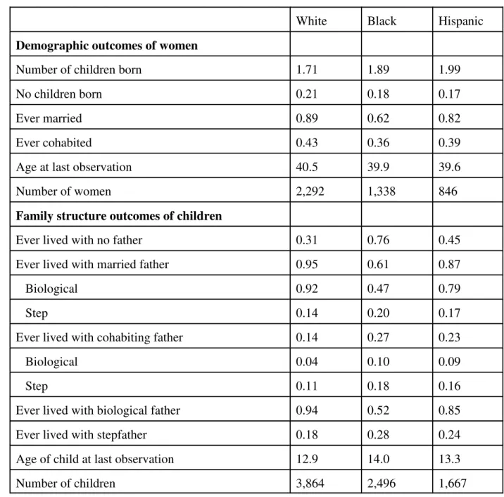
a sample of 4,476 women out of 4,926 eligible for inclusion.15 _{Descriptive statistics on the} analysis sample are displayed in Table 1, separately for whites, blacks, and Hispanics. The first

panel summarizes outcomes of the demographic processes modeled here, as of the last interview.

who were interviewed in 2004 were between the ages of 39 and 47.

had given birth to an average of 1.71 children, and 21% had not given birth to any children. Black and Hispanic women had about 0.2 to 0.3 more births on average than whites. Eighty nine

percent of white women had ever been married, compared to 62% of black women and 82% of Hispanic women. White women were also somewhat more likely to have ever cohabited.

The lower panel of Table 1 summarizes the incidence of the family structure outcomes experienced by the 8,027 children born to the sample women as of their last interview. The

children were aged 13-14 on average at the time of the last observation (after truncating at age 18; without truncating, they were 14-16). Thirty one percent of children of white mothers had

ever lived without a father figure present, compared to 76% of the children of black mothers and 45% of the children of Hispanic mothers. Most children of white and Hispanic mothers lived

with both biological parents at some point in their childhood (94% and 85%, respectively), compared to 52% of the children of black mothers. Children of black mothers were more likely

to live with a stepfather and/or a cohabiting father compared to children of white and Hispanic mothers, but these differences are smaller.

A concern with using a long panel for a study of family structure is that attrition and immigration could make the sample increasingly unrepresentative over time. Most studies of

family structure use a time series of cross sections, and do not face this problem, although they cannot study individual-level dynamics with such data. To examine this issue we compared summary statistics for the NLSY79 cohort in the NLSY79 data and the March Current

Population Survey (CPS), for two years, 1995 and 2004. 1995 is the first CPS survey year in which cohabitation is well-measured, and 2004 is the last year of data in our NLSY sample. The

results are shown in Appendix Table A-1. Panel A shows close agreement on union status

between the two data sources for whites in 1995, with a bit more disparity by 2004. For example,

the percent single in 1995 was 21.9 in the NLSY and 20.2 in the CPS, while in 2004 the figures were 22.3 and 18.3, respectively. The NLSY estimate of percent single for blacks differs by 4

percentage points from the CPS, increasing to 8 percentage points by 2004. The NLSY-CPS difference in percent single for Hispanics is 7 percentage points in 1995 and 6 percentage points

in 2004. The percent of Hispanic women cohabiting in 1995 is 8.1 in the NLSY versus 2.1 in the CPS, although the gap is only one percentage point in 2004. The largest disparity for Hispanics is

14 percentage points for percent married in 1995, shrinking to 7.5 percentage points in 2004. It is plausible that the largest disparity would be for Hispanics, since the bulk of immigrants in the

last 30 years were Hispanic. Panel B shows that mean years of education for whites and blacks are very close in the NLSY and CPS, but over one year higher in the NLSY compared to the CPS

for Hispanics. This pattern is likely due to lower education among recent Hispanic immigrants compared to Hispanics present in the U.S. in 1979.

Panels C and D show close correspondence in the number of children present in the woman’s home by age group, and the fraction of women with no children in the home. Panel E

shows that the distribution of children by the mother’s union status is quite a bit closer between the NLSY and CPS than is the distribution of women by union status. The CPS does not identify biological versus step children, so this comparison cannot be made. Finally, Panel F shows that

the percent of children with no father present is remarkably close in the two data sets. Overall, the NLSY79 sample has not been compromised by attrition, but is increasingly unrepresentative

17_{TANF was implemented by all states, while not all states requested a welfare waiver.} TANF incorporated many of the rule changes implemented by various states as part of their waivers, including time limits and welfare-to-work (workfare, learnfare) programs. TANF was implemented by states between 1996 and 1998. See Figure 1B for the aggregate timing pattern.

B. Contextual Data

The geo-coded version of the NLSY79 provides the state of residence at each survey date,

and at the time of the woman’s birth and when she was age 14. We collected data from a variety of sources on welfare benefits, welfare reform, divorce laws, tax rates, and labor market

conditions, and merged them with the NLSY79 data by state and year. Here we briefly describe the key measures; Appendix B provides details, and describes how state of residence was

assigned for non-survey years.

The real (year 2000 dollars) Aid to Families with Dependent Children (AFDC) or

Temporary Assistance for Needy Families (TANF) plus Food Stamp benefit for a family of four (single mother with three children under 18) with no other income is used as a measure of the

welfare benefit. The average welfare benefit declined in real terms over much of the sample period, with a couple of episodes of relative stability (see Figure 1A). The month and year of

implementation of major welfare waivers and the TANF program for each state are used to characterize welfare reform. The welfare reform variable indicates the presence of any major

change in welfare rules authorized by a waiver or TANF.17

The month and year of enactment of unilateral divorce laws were taken from Gruber

(2004), which is an update of Friedberg’s (1998) data. Unilateral divorce means that mutual consent for a divorce is not required. Most such laws were enacted in the 1970s, but there were occasional later cases in which states passed a unilateral divorce law (Figure 1C).

The TAXSIM program provided by the National Bureau of Economic Research (NBER) was used to compute the average tax rate for alternative filing statuses and numbers of children.

The program accounts for all major features of the tax code, including the EITC and (beginning in 1977) state taxes. Rather than conditioning on the woman’s observed income, we specify an

arbitrary real income level that is used for all women in all years. This ensures that the only variation in the tax rate used in the model is due to tax code variation over time and across states.

In the results reported here, we used the real equivalent of the year 2000 poverty line for a family of three. We estimated an alternative specification using the real equivalent of year 2000 median

family income, and found similar results. The average tax rate is a better characterization than the marginal tax rate for the implications of alternative discrete marriage and childbearing choices.

The tax rate is treated as a choice-specific variable that depends on the marital status and number of children associated with each alternative a woman faces. For example, the alternatives

available to a married woman with one child are to remain in this state, conceive a second child, or end the union and become single. The tax rate is different for each alternative: married filing

jointly with one child, married filing jointly with two children, and head of household with one child, respectively. Marital status and number of children are outcomes of the choice processes

and therefore endogenous if there is serially correlated unobserved heterogeneity. Conditioning on the permanent woman-specific effect (µi) and integrating it out of the likelihood function accounts for this source of endogeneity if the heterogeneity is permanent. Thus, in our analysis,

the tax rate varies over time, across states, and by fertility and marital status. There was rapid growth in the tax subsidy to children for low-income women beginning in the 1980s (see Figure

18_{In addition to the contextual variables, the specification includes black and Hispanic} indicators, a quadratic in the woman’s age, the number of children fathered by the current man, the cumulative number of cohabitations, whether a single woman was in a cohabitation or a almost exclusively to low-income families with children (and is refundable, hence the possibility of a negative average tax rate).

The female wage rate is measured by the mean real full time average hourly earnings of women aged 16-47. The state-year-specific mean wage rate is constructed separately for whites,

blacks, and Hispanics using data from the Current Population Survey (CPS) by dividing weekly earnings in the survey week by hours of work per week. The age group 16-47 spans the

(employment-eligible) age range of the NLSY sample in the years for which we have data. In order to avoid introducing composition effects into the wage trends, we regression-adjust wages

for education and age. The wage measures used here are standardized to a constant level of education (high school graduate) and age (26-30). The male wage rate is constructed in the same

way, for a sample of men aged 18-49. Note that the wage rate is not choice-specific: it is not conditioned on marital status or fertility. It is also not conditioned on the education or other

human capital characteristics of the women in our sample. Figures 1E-1G show that the male-female wage gap narrowed for all three groups through the mid 1990s, especially for Hispanics,

but has been relatively constant more recently. In absolute terms, only for white and Hispanic women are mean real wages higher in 2004 than in the 1970s.

5. Results

The parameter estimates and standard errors on the policy and labor market variables are

marriage in her previous spell, quadratics in the ages of her youngest and oldest children, and quadratics in the duration of cohabitation and single spells. See Appendix Table A-3 for the parameter estimates on these variables. In the interests of empirical tractability we imposed a substantial number of exclusion restrictions in cases in which a given variable consistently had small and statistically insignificant effects. In alternative specifications, we found that the mother’s date of birth, number of marriages, total number of children, duration of marriage, and duration of pregnancy could be excluded with little impact on the predictions of the model. The estimates of the factor loadings and probability weight shown in Table A-3 are jointly highly significant, and imply a plausible correlation structure among the disturbance. For example, the disturbance in the union dissolution alternative (choice 3) is negatively correlated with the other disturbances, indicating that unobserved factors that increase the likelihood of ending a union are negatively correlated with unobserved factors that increase the propensity to enter a union and bear children. The correlation between the disturbances in the conceive- a- child- with- a- new-man and marry- a- new- new-man alternatives is 0.46.

we do not discuss them. The specification reported here includes the six contextual variables described above, each interacted with indicators for black and Hispanic, thus allowing the effects

to differ freely by race/ethnicity. The specification also includes dummies for nine census regions and the 22 largest states, a quadratic in calendar time, dummies for five (or in some cases ten)

year periods, and dummies for several individual years in the mid 1990s, around the time of welfare reform. The model is nonlinear and has a large number of parameters. Given the

relatively small numbers of women from the less-populated states, as well as the low frequency with which some alternatives were chosen in some of the calendar years, it was not feasible to

incorporate full sets of state fixed effects and calendar year fixed effects, leading us to group some of them together instead. The geographic and time controls are included in order to avoid

attributing the effects of unobserved differences across states and over time to the contextual variables of interest. However, the geographic controls also absorb the true effects of permanent

cross-state differences in the contextual variables, as well other permanent differences across states, thus leaving only variation over time around state-specific averages to identify the effects

19_{The simulated data for children are truncated at age 18. As in the data, some children are} not observed for their entire childhood in the simulations, because they have not reached age 18 in the last period in which the mother is observed. In the simulations, there are no deaths, no twin births, and no cases in which children move in or out of the mother’s household.

of the contextual variables (Keane and Wolpin, 2002). Below, we discuss the sensitivity of the results to specifications with alternative sets of geographic controls.

We use the parameter estimates to simulate the life history of each woman in the sample. The simulations condition only on the woman’s race/ethnicity, age, and the state of residence in

each year in which she is observed. A woman is assigned a heterogeneity type (a value of µ) based on a draw from the estimated heterogeneity distribution. Each woman starts out single and

with no children at age 12. The estimates are used to compute the probability of each of the three events in the choice set in this case (enter a cohabitation, enter a marriage, conceive a child),

given her type (µ), race/ethnicity, and state of residence at age 12. A random number generator determines which, if any, event occurs. If the event is conceiving a child, a pregnancy duration is

randomly assigned by drawing from the observed distribution of pregnancy durations in the sample. The Y_it variables are updated according to which event, if any, occurred, and the process

is repeated for the next month. If pregnant, the birth occurs at the assigned duration. The simulation continues through the last month in which the woman is observed in the data.19 _This

procedure is repeated 100 times for each woman. To generate standard errors for the simulations, we took 200 random draws from the joint distribution of the parameter estimates, and repeated

the entire simulation procedure for each draw. We report the mean and standard deviation of the resulting simulations.

A-20_{Tables A-4 and A-5 use the actual parameter values rather than drawing from the} parameter distribution, so no standard deviations are reported.

4 in the Appendix compares simulation results for selected variables characterizing choice behavior to the observed values in the data.20 _{The model reproduces most aspects of the data}

reasonably well, but under predicts the proportion of childhood living without any man present. Table A-5 illustrates the fit of the model to transitions of children among the five family structure

categories of interest. This is a demanding measure of fit, since these transition probabilities are not directly estimated, but rather are derived from the underlying transition probabilities of

women among states. The upper panel compares simulated and actual transition probabilities averaged over all ages from 0 through 17. The model fits the transition probabilities very well in

some cases, such as transitions involving a man entering the household (rows 1-4), breakup of cohabitations and marriages with stepfathers (rows 7 and 10). The simulations underestimate the

rate of dissolution of marriage to the biological father (row 9), and overestimate the rate at which cohabitations are converted to marriages (rows 6 and 8) and the rate at which cohabitations with

the biological father break up (row 5). The fit averaged over ages 0-5 shown in the lower part of the table is similar to the fit average over all ages.

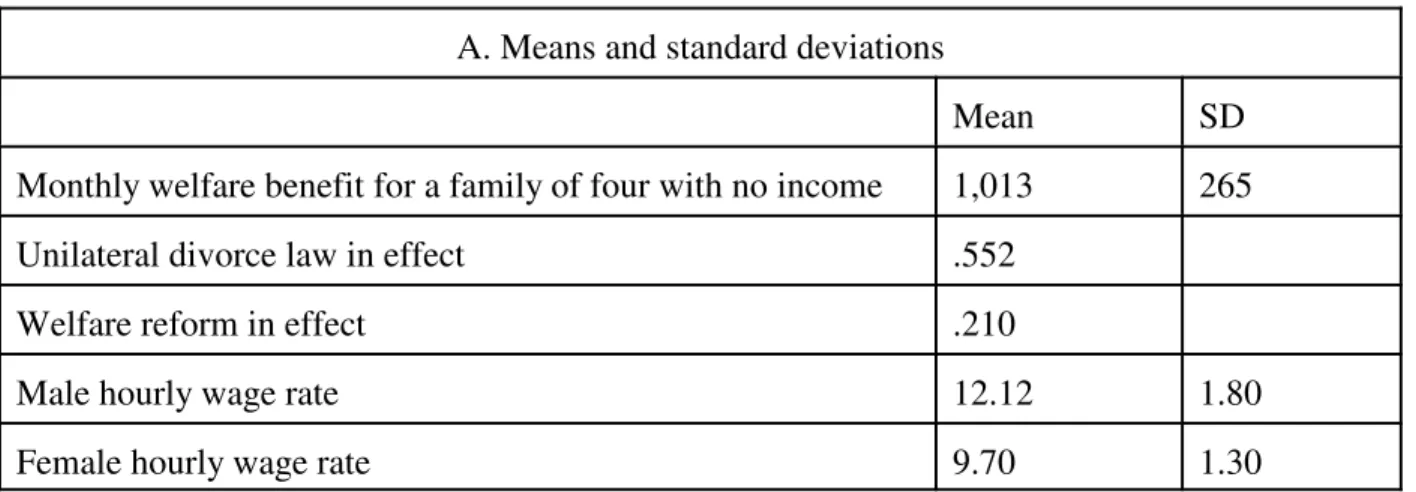
To illustrate the effects of wage rates and the welfare benefit, we compare two scenarios (separately for each variable): one in which the variable is held constant for all women and all

periods at its overall sample mean, and another in which it is held constant at the mean plus one standard deviation. For the tax rate we compare one scenario in which the tax rate for each combination of marital status and number of children is held constant at its sample mean to three

21_{From Table 2, a one standard deviation increase in the wage rate is a 13.4% change. The} baseline simulated proportion of childhood spent living with no father is 0.33 for blacks and 0.12 for Hispanics (see Appendix Table A-3). The simulated change of 0.060 for blacks in Table 3 is an 18.2% increase over the baseline value, yielding an elasticity of 1.36 = 18.2/13.4. For

Hispanics, the corresponding elasticity estimate is 3.64 = 47.5/13.4.

which the tax gain from having children conditional on marriage is eliminated; and a third in which the tax gain from having children conditional on being unmarried is eliminated (see the

notes to Table 2 for details). For welfare reform and unilateral divorce, the two scenarios hold the variable constant at zero and at one. The values of the contextual variables used in the

simulations are shown in Table 2.

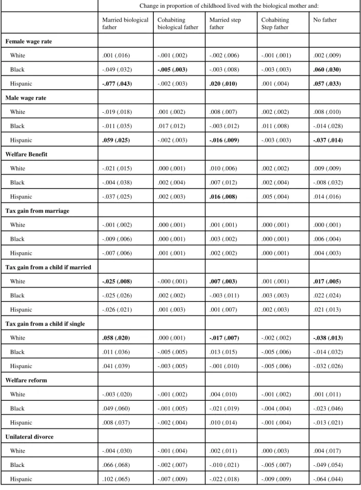
Table 3 shows simulated effects of the contextual variables on the proportion of

childhood spent in the five family structures of interest. The results show that an increase in the average female wage rate causes an increase in the proportion of childhood spent living with no

father. The effect is very small for children of white mothers, but is large for children of black and Hispanic mothers. The implied wage elasticities of the proportion of childhood spent with no

father are 1.36 for children of black mothers and 3.64 for children of Hispanic mothers.21

Another way to illustrate the magnitude of these effects is to note that the mean real wage rate of

black women fell by more than one standard deviation, from over $10 to $8.50, from the mid 1970s to the early 1990s (see Figure 1). The results in Table 3 imply that this decline would have

reduced the proportion of childhood spent with no father by more than 0.06, from a baseline of 0.33. Most of the increase in the proportion of childhood spent living with no man comes at the

expense of time spent with the married biological father.

The effects of an increase in the male wage rate are almost all opposite in sign to the effects of an increase in the female wage rate. This is consistent with the prediction of Becker’s

model of specialization in marriage. The simulated effects are small for children of white and black mothers. For children of Hispanic mothers an increase in the male wage causes a decline in

time spent with no father and with a married step father, accompanied by an increase in time spent living with the married biological father. The decline of .037 in the proportion of childhood

spent with no father is quite large relative to the baseline of .122 for children of Hispanic mothers.

These hypothetical exogenous changes in average market wage rates affect behavior presumably because the wage offers available to individuals in our sample are drawn from the

corresponding market wage distributions. The estimates can be interpreted as reduced form effects, showing how changes in average market wages affect family structure without

identifying the underlying mechanisms of the effects. Thus we cannot identify how an increase in the mean wage offer affects the distribution of wage offers by skill or ability, nor the effect of

wage offers on employment decisions. The advantage of the approach is that it is feasible to estimate the net impact of wages on all of the demographic behaviors that determine family

structure.

An increase in the welfare benefit is estimated to cause a decrease in the proportion of

childhood spent living with the married biological father for all three groups, but the estimates are not significantly different from zero. The negative effect is consistent with the predictions of economic models of the family (e.g. Neal, 2004; Willis 1999). The decrease is accompanied by

an increase in time spent living with no man (except for blacks) and cohabiting men, but the proportion of childhood spent living with a married step father also increases.

22_{The simulation of the effects of the tax gain from an additional child within marriage} holds constant the tax gain from an additional child outside of marriage, and vice versa. Further examination of these effects would require an analysis of income and substitution effects (both within and across periods) of the tax gain on labor supply and earnings. Note that in a household bargaining model with divorce and child support transfers, the impact of an EITC-type tax credit, which is especially beneficial to single mothers, on divorce has an ambiguous sign (Francesconi et al., 2007).

in the sense that we can reject large effects with considerable confidence. The simulated effects of the tax gain from having children conditional on being married are also quite small in most

cases, but a few of the effects are a bit larger. It is surprising that the tax gain from children conditional on marriage is estimated to cause a decrease in the proportion of childhood spent

living with a married father, by about 0.025 for all three groups, accompanied by an increase in time spent living with no father. This is a puzzling finding, and is robust across the alternative

specifications we have estimated. The simulated effects of the tax gain from children conditional on being unmarried are also counterintuitive, resulting in an increase time spent with the married

biological father and a decline in time spent with no father present.22

The last two panels in Table 3 show the simulated effects of welfare reform and unilateral

divorce. The simulations reveal some moderately large effects in a few cases, but none are significantly different from zero. Welfare reform is estimated to cause an increase of .049 in the

proportion of childhood lived with the married biological father for children of black mothers. Unilateral divorce also causes a rather large increase in the proportion of childhood living with

the married biological father for children of black and Hispanic mothers. The lack of precision of these estimates is probably due to the fact that most of the changes in unilateral divorce laws

were in the early 1970s (see Figure 1C), so these changes affected relatively few individuals in our sample during the prime childbearing years. Welfare reform occurred in a fairly narrow time

span from the late 1980s through 1997 when the NLSY79 cohort was in their 30s, past prime childbearing ages.

Family structure changes are thought to have different effects on children in different stages of childhood (e.g. Hill et al., 2001; Moore et al. 2001). We examined whether the effects

shown in Table 3 were concentrated in particular phases of childhood: early (0-4), middle (5-11), and late (12-17). These are hypothesized by developmental psychologists to be distinct stages in

the developmental life course. The results (not shown) do not indicate any systematic tendency for the effects to be concentrated in particular stages of childhood. In a few cases, the effects are

stronger at younger ages (e.g. welfare reform for blacks), while in a few other cases the effects are stronger at older ages (e.g. tax gain to having children for whites). In the great majority of

cases the effects are quite similar across the age groups.

The outcomes shown in Table 3 are measures of the “stock” of time spent in alternative

family structures. It is of considerable interest to investigate the underlying determinants of these stocks, which include both a child’s family structure at birth, and “flows” of men in and out of a

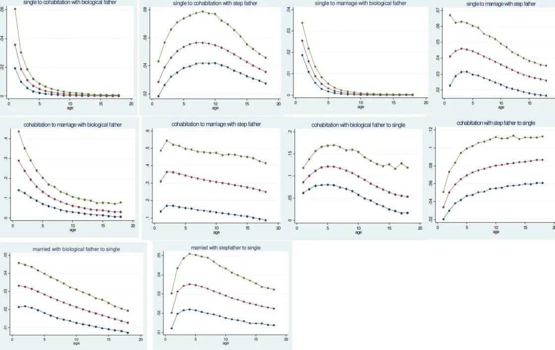
child’s household. Consider the effect of a one standard deviation increase in the female wage rate, which was estimated to cause an increases of 0.060 and 0.057 in the proportion of childhood

living with no father for children of black and Hispanic mothers, respectively. The simulated increase in the probability that the mother was single at the birth of the child is 0.038 (se 0.035) for blacks and 0.056 (se 0.031) for Hispanics, accounting for a substantial part of the increase in

the proportion of childhood living with no father (not shown). Figure 2 shows the simulated effects of the wage increase on annualized transition rates of children of black mothers among

of marriage increase by .02 to .03, thus contributing to the increase in time spent with no father. Cohabitations break up at a more rapid rate as well. Surprisingly, transitions into cohabitation

and marriage also increase. The corresponding effects for children of Hispanic mothers (not shown) are all in the same direction, but smaller and less often significantly different from zero.

Another interesting finding in Table 3 is the negative effect of a higher male wage rate for children of Hispanic mothers on the proportion of childhood living with no father (-.037), and the

increase in time spent living with the married biological father (.059). The simulated effect of an increase in the male wage rate on the probability that the mother was single at the birth of the

child is -.046 (se .023) for children of Hispanic mothers, which can account for all of the -.037 change in the proportion of childhood spent with no father. Changes in transition rates contribute

little in this case (not shown).

We now use the estimates to address a different question: how did the observed trends in

the contextual variables affect family structure, compared to a counterfactual scenario in which the contextual variables remained constant at their state-and-race/ethnicity-specific 1970-1974

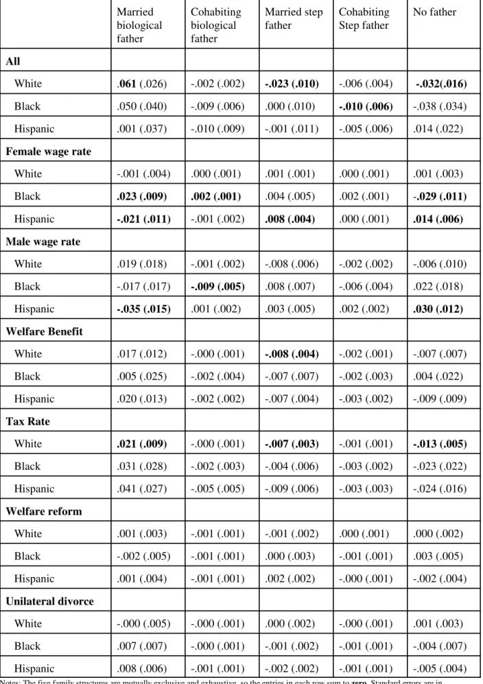
means, the values that prevailed when the NLSY79 cohort of women was entering adolescence. The first panel of Table 4 shows the simulated impact of exposure to the observed values of the

contextual variables compared to the counterfactual in which they all remained at their early 1970s levels. For children of white mothers, the simulations imply that changes in the contextual variables caused an increase in the proportion of childhood spent with the married biological

father of 6.1 percentage points, and decreases of 2.3 percentage points in time with a married step father, and 3.2 percentage points in time spent with no father. These are moderately large effects,

married step father, and 7% with no father (see Appendix Table A-3). The simulated effects for the children of black mothers are similar in sign and magnitude, but are not as precisely

estimated. The effects for Hispanics are substantially smaller. These results imply that if the contextual variables had remained at their early values during the past 30 years, the proportion of

time children lived without their biological father (or without any father) would have been even larger than the observed proportions.

The remaining panels of Table 4 show the effects of changing one variable at a time. An important source of the total effects for whites and blacks is the change in the average tax rate,

which declined substantially for families with children beginning in the mid 1980s. This was reinforced by a declining female wage rate for blacks. For whites, the decline in the welfare

benefit also contributed to the observed changes. For Hispanics, female and male wage trends that both caused less time spent in marriage and with the biological father were offset by the

effects of trends in tax rates and welfare benefits. Because female and male wage rates tend to move in the same direction and have opposite effects on most behaviors, the relatively large

effects of both male and female wages for blacks and Hispanics shown in Table 3 tend to cancel each other out. The effects of welfare reform and unilateral divorce are negligible for all three

groups, not surprising given the small estimates in Table 3.

The final issue considered here is whether the model can explain the large changes in family structure in recent decades in the U.S. There are no consistent time series available from

the 1970s onward on children living in cohabiting arrangements and on biological versus step fathers, so the only trend we can analyze is the proportion of children living with the mother

of the observed trend in the proportion of children living with no father from the early 1970s through the early 2000s can be explained by our model: in one case we hold all the contextual

variables constant at their 1970-1974 state-race/ethnicity-specific means, and in the other case we hold them all constant at the corresponding 2000-2004 values. Comparing the two simulations

gives an estimate of the effect of the observed changes in contextual variables on the proportion of childhood spent living with no father.

Table 5 uses CPS data to show that the proportion of children living with no father increased from 0.095 to 0.191 for whites from 1970-74 to 2000-04, and from 0.388 to 0.572 for

blacks. For Hispanics, the time series begins in 1980, and there was a small increase from 0.253 to 0.278 from 1980-84 to 2000-04. The table shows that our simulations cannot explain any of

the observed change for whites, and only a very small proportion for blacks. The simulations over-predict the magnitude of the increase for Hispanics, but it is not clear how much weight to

put on this, given that the composition of the Hispanic population is changing over time, while the NLSY79 Hispanic sample is representative only as of 1979. One other series available on a

consistent basis is the fraction of those children living with no father whose mother has never been married. Table 5 shows that this increased from 0.086 to 0.417 since the early 1970s, a

change of 0.331. The observed changes in the contextual variables predict an increase of 0.037, only about one tenth of the observed change. Thus, as in much previous research, our estimates indicate that the economic and policy variables we considered contributed little to the observed

changes in family structure.

23_{The entries in column 1 of Table 6 differ slightly from the corresponding entries in} Table 3 because the results in Table 6 use the actual point estimates of the parameters rather than 200 draws from the parameter distribution as in Table 3.

The results discussed above are based on a specification with a rich set of controls for fixed geographic effects: 22 state dummies and nine census division dummies. As discussed

above, this specification has the advantage of controlling for unobserved differences across states and census divisions that could be correlated with the contextual variables. The source of

identification is variation in specific trends in the contextual variables around the state-specific means. In order to determine whether the results are sensitive to the source of

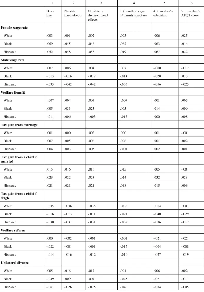
identification, we re-estimated the model with two alternative specifications: one that drops the state fixed effects, and one that drops the nine division dummies as well. Table 6 shows the

simulated effects of the contextual variables on the proportion of childhood spent living with no father, for alternative model specifications. Column 1 reproduces the results for the main

specification, from the last column of Table 3.23 _{Columns 2 and 3 report results from the new} specifications. Most of the simulated effects are very similar, suggesting that responses to

permanent differences across states are similar to responses to variation around means within states. There are a few notable differences, however: the effect of the welfare benefit for blacks

changes from 0.005 to 0.031; the effect of welfare reform for blacks changes from 0.022 to 0.001; and the effect of unilateral divorce changes from 0.049 to 0.009 for blacks and from

-0.061 to -0.026 for Hispanics.

Another important feature of the specification is the absence of controls for the

characteristics of women, other than race/ethnicity. The effects that we attribute to the contextual