Pensions, Labor, and Individual Choice

(1)

This PDF is a selection from an out-of-print volume from the National Bureau

of Economic Research

Volume Title: Pensions, Labor, and Individual Choice

Volume Author/Editor: David A. Wise, ed.

Volume Publisher: University of Chicago Press

Volume ISBN: 0-226-90293-5

Volume URL: http://www.nber.org/books/wise85-1

Publication Date: 1985

Chapter Title: Social Security, Health Status, and Retirement

Chapter Author: Jerry A. Hausman, David A. Wise

Chapter URL: http://www.nber.org/chapters/c7133

Chapter pages in book: (p. 159 - 192)

(2)

and Retirement

Jerry A. Hausman

David A. Wise

As people age they would like to work less. We observe, however, that for most persons, retirement is abrupt. The typical person retires from a job at which he was working full time, although many work part time on another job after retirement. Because retirement is a discrete outcome, it is natural to think of it in a qualitative choice framework. But retirement also has a time dimension, age, which not only characterizes retirement but affects the desire for it as well. Thus it is natural to describe retirement within the context of a continuous time qualitative choice model. In this spirit, we pursue a probability model of time to retirement (age of retirement).

We shall begin with a failure rate or hazard model specification common in the statistical and biometric literature (see Cox 1972 or Kalbfleisch and Prentice 1973, for example). Such a model was recently used by Lan- caster (1979) to describe the duration of unemployment. Our model paral- lels his, with some slight extensions.' This model is essentially a reduced- form specification. In particular, it seems to have no natural utility maximization or first choice interpretation common to qualitative choice models in the econometric literature (e.g., McFadden 1973; Hausman and Wise 1978).

We then pursue another continuous time model of retirement that we hope will ultimately lend itself to a more structural interpretation but which also maintains the advantages of the hazard model. The central idea is to specify disturbances that follow a continuous time Brownian Jerry A. Hausman is professor of economics, Massachusetts Institute of Technology, and research associate, National Bureau of Economic Research. David A. Wise is John F. Stam- baugh Professor of Political Economy, John F. Kennedy School of Government, Harvard University, and research associate, National Bureau of Economic Research.

We are grateful for the extensive research assistance of Andrew Lo, Douglas Phillips, Lynn Paquette, and Robert Vishny.

(3)

160 Jerry A. HausmadDavid A. Wise

motion (or Wiener) process. (See, e.g., Cox and Miller 1965; Karlin and Taylor 1975.) This leads to retirement likelihoods that have much in common with probit qualitative choice models while capturing the continuous time hazard idea as well. The specification of this model as we have set it up differs substantially from the hazard model. In particular, we make ex- plicit use of hours worked before retirement, a consideration that plays no role in the hazard model. To date, however, the specifications of this model have not yielded entirely plausible results. We present the model none- theless, in the hope that our experience will be of interest to others facing similar problems.

Empirical analysis is based on the Longitudinal Retirement History Survey (LRHS). The survey began in 1969 with over 11,000 persons who were aged 58-63 at that time. A series of follow-up surveys were used to obtain information on these persons at two-year intervals through 1979. We use all six surveys. The LRHS provides detailed labor supply, social security, earnings, health, and other information about those surveyed. To motivate the development below, we shall have in mind observations on each individual at selected ages.

The empirical focus of the paper is the effect of health and social security wealth, or social security payments, on retirement. Labor force participation fell significantly during the period of our data; the participation rate of men fell particularly substantially. The rates for 60-64-year-olds and those 65 between 1969 and 1979 were as shown in the unnumbered table below. Year 60-64 65

+

1969 75.8 27.4 1971 74.0 26.3 1973 68.9 23.4 1975 65.4 21.9 1977 62.6 19.9 1979 61.1 20.3

Part of this decline may have resulted from real increases in social security benefits, at least between 1969 and 1975. But counteracting influences were provided by increased real earnings during the beginning of the period and by large increases in future social security benefits from continued work. This latter effect has been emphasized by Blinder et al. (1980). Our models attempt to distinguish the effects of these influences.

The estimates based on both of the models that we use suggest a strong effect of social security benefits on the probability of retirement, with the increase in benefits between 1969 and 1975 accounting for possibly a 3%- 5% increase in the probability of retirement for men 62-66. Both models suggest that increases in real earnings decrease the probability of retire-

(4)

ment. Results based on the hazard model indicate that increases in future social security benefits decrease the probability of retirement, while the initial results of the Wiener model suggest the opposite. Because the Brownian motion model is in the early stages of formulation and the results are preliminary, it may be premature to attempt to explain the differences in results.

We begin by setting forth the hazard model. Then we present descriptive statistics that help motivate our specification of this model. For con- venience, we also present data that help to understand our formulation of the Brownian motion alternative. After presenting estimates based on the hazard model, we describe a continuous time model of retirement based on a Brownian motion process and then present initial estimates based on this model.

6.1 The Proportional Hazard Approach 6.1.1 The Model

Suppose the probability that a person has retired by age t is given by

where 8

>

0. This is a convenient probability specification with the intu- itive property that the probability of retirement goes to one as t gets large. For example, if 8 were a function only of age, with 19 ( t ) = f(t) = t " - l / a , a

>

0, then G(t) would be 1

-

exp[t"/c~~]-~, with exp[*]-' going to zero as t increases. Note thatf(t) is increasing with age if a

>

1 and decreasing with ageif0

<

CY

<

1.

Associated with this "cumulative distribution" function is the density function

describing the likelihood of retirement at ages t (0

<

t

<

a). The "instantaneous" hazard rate describes the conditional likelihood of retirement at age t , given that the person has not retired before t. It is simply

(3)

To make the distribution function G(t) a function of individual attributes, the instantaneous hazard rate 8 is parameterized in terms of attributes X, in this case including age itself. For expository purposes, it is useful to develop the specification in stages. Suppose first that 8 is a function of age t and of individual attributes X I that do not change with age such

(5)

162 Jerry A. Hausman/David A. Wise

that 8(t) = exl@-f(t) = exI@I.P-I/a, where

PI

is a vector of parameters and XI a vector of attributes. In this case, the probability of being retired by age t is G(t) = 1 - exp[exI@I * P / a 2 ] - I .

Now suppose that there are unobserved as well as observed determi- nants of retirement. A convenient way to allow for unobserved individual attributes is to specify a random individual-specific term v that enters 8 such that

(4) 8(t) = v.exl@I.P-l/a.

Note that v is time invariant; it simply induces a proportional shift in the hazard function 8( a ) over all values of age t. The same is true for differences in XI.

If we assume that v has

a

gamma distribution over individuals (0

<

v

<

m), we can obtain a closed-form solution for G(t).3 In particular, the probability that a person with attributes XI has retired by age t is given by

with the last term obtained after some manipulation. Although this expression is not defined for a2 = 0, as the variance goes to zero, G(t;XI) goes to 1

-

exp($l@.P/a2)-I, the result with no random term.

Finally, suppose that there are some measured individual attributes Xz that change with age. We again specify 8 in a separable manner as

(6) 8(t) = u-ex1@1.X2(t).f(t)

.

(7) G ( ~ ; x ) = 1 - [I

+

u2exp(XIPI)

.

x2(7) * f(7)d~i

.

Now the probability of retirement by age t becomes

The specification is completed by describing the integral

(8) Os'X2(7) 'f(7)dT

.

Since we do not have continuous observations on X2, which would presumably allow integration over the function X2(t) determined by such

a

path, we specify the integral using the piecewise linear formulation

0s' X~(T)

-

f(7)d7 =

2

g2@ ) P 2

-

Yg\f(7)d7

,

(9)

where p denotes the period. For example, p = 0 indicates the period between age 54 and the age at the time of the first survey, p = 1 indicates the period between the first and second survey, and so on. Note that 54 is tak-

(6)

en as an arbitrary starting point, implicitly assuming that no one would have retired before this age. The variable %(p) is the average of

XZ

during period p , and to@) and t,@) are the initial and final ages, respectively, of the person during period p . (A discretely changing variable, like married or not, is taken to be the value of the variable the next time it is observed. If the variable is continuaus, like income, the average is obtained by assuming that the variable followed a linear path over time.) We can also alter the specification of 0 to allow for a discontinuous jump in the hazard rate at any age t . For example,

X I

can include dummy variables that assume nonzero values at particular ages.

Given 0 ( t ) and G(t), it is straightforward to specify the likelihood of a variety of sample observations (see, e.g., Lancaster 1979). In particular, in our case there are three possibilities: the person was retired when first surveyed at age t( 1) with corresponding probability G[t(l)], the person had not retired by the last (Nth) survey period at age t(N) with probability

1 - G [ t ( N ) ] , or the person retired between the nth and mth surveys, when he was aged

t(n)

and t(m), respectively, with probability G[t(n)]

-

G[t(m)]. The likelihood function obtained from these terms may be maxi- mized to obtain estimates of the coefficients /3 on the variables X and on age, as well as the variance u2 of u .

6.1.2 Some Descriptive Statistics

Before we discuss estimates based on this model, we shall present sum- mary statistics that help to motivate the model and our particular specification of it. Although our estimates are based on non-self-employed males, for comparative purposes, we also present descriptive data for self- employed men and for women. Empirical hazard rates for non-self-employed men are shown in table 6.1, by age and survey year. Tables 6.2 and

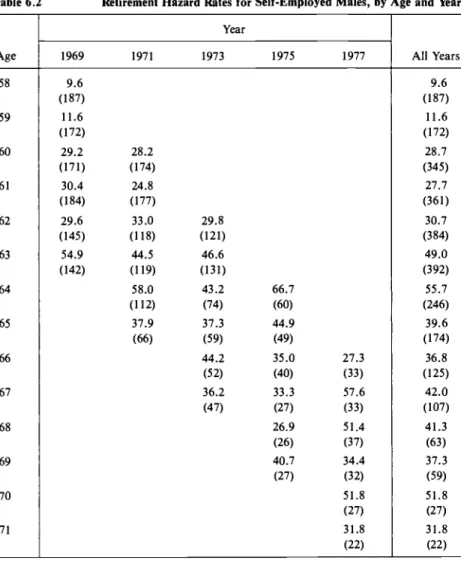
6.3 contain analogous data for self-employed men and for women, respectively. These data show the proportion of those not retired in a given year who retired during the next two-year interval. First we observe that the pattern of rates for self-employed men is quite different from the pattern for the non-self-employed. In particular, the jump at age 62 is much less pronounced for the self-employed, and the rates thereafter are much lower. The rates for women, however, are not strikingly different from those for men. This suggests that the availability of social security at 62

for the non-self-employed may play a substantial role in retirement behavior.

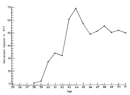
The hazard rates for men are graphed in figure 6.1. While the rates increase rather smoothly to age 62, we observe substantial jumps between ages 63 and 65 and then very little increase in the hazard rates after 65. This pattern would appear to be inconsistent with a hazard rate 0(t) = f(t)

= t"-'/a that depends only on age and is always increasing in age for a

>

1 . Thus we allow the hazard rate O( - ) to depend on individual attributes X,

(7)

Table 6.1 Retirement Hazard Rates for Non-Self-Employed Males, by Age and Year

Year Age 58 59 60 61 62 63 64 65 66 67 68 69 70 71 1969 1971 1973 1975 1917 30.5 (662) (723) 34.8 (604) (534) 72.9 (480) 58.9 (236) 36.2 64.6 33.9 (445) 60.3 (438) 68.1 (398) 56.7 (701) 45.8 (144) 52.6 (116) All Years 10.7 (782) 12.0 (872) 27.2 (1488) 34.2 (1542) 32.3 (1766) 60.7 (1518) 69.2 (1119) 57.3 (630) 49.0 (404) (3 13) 55.4 ( 166) 50.4 (125) 52.0 50.0 (32) 51.4 (50)

Note: The hazard rate in year t is the ratio of the number of people who retire between years t

and t

+

2 to the number of nonretired people in year t, in percent. Numbers in parentheses are numbers of observations used to calculate hazards.

as well as on age. In particular, this pattern motivates the assumption of the unobserved random terms u that induce proportional shifts in the hazard rate, given

X

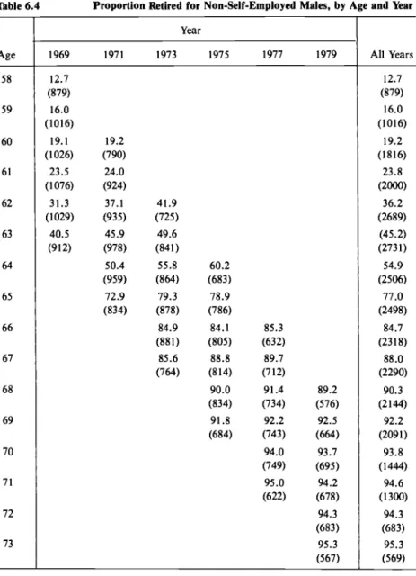
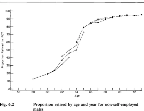
and t.

The percentage of non-self-employed men that is retired is shown in table 6.4 and for each age and year. Figure 6.2 presents the same data graphically. The most striking feature of these data is the very marked increase between 1969 and 1973 in retirement rates of men 62-65. For example, 31% of 62-year-olds were retired in 1969; by 1973, almost 42% of this

(8)

Table 6.2 Retirement Hazard Rates for Self-Employed Males, by Age and Year Age 58 59 60 61 62 63 64 65 66 67 68 69 70 71 Year 1969 1971 1973 1975 1977 9.6 (187) 11.6 (172) 29.2 (171) 30.4 (184) 29.6 (145) 54.9 (142) 29.8 (121) 46.6 (131) 43.2 (74) 37.3 (59) (52) 36.2 (47) 44.2 66.7 (60) 44.9 (49) 35.0 (40) 33.3 26.9 (26) 40.7 (27) (27) 27.3 (33) 57.6 (33) 51.4 (37) 34.4 (32) 51.8 (27) 31.8 (22) All Years

Note: The hazard rate in year t is the ratio of the number of people who retire between years 1 and t t 2 to the number of nonretired people in year t, in percent. Numbers in parentheses

are numbers of observations used to calculate hazards.

age group were retired. Note that the limited evidence provided in these data suggests little change in retirement rates after 1973. About 79% of 65-year-olds were retired in both 1973 and in 1975.

The estimates we present below depend in part on our definition of retirement. We assume that a person is retired when he says that he is fully or partially retired. Although this may seem an obvious choice, on reflec- tion, it becomes clear that retirement status is ambiguous. For example, our definition does not correspond to zero hours of work. While many

(9)

166 Jerry A. HausmadDavid A. Wise ~~ ~~ ~

Table 6.3 Retirement Hazard Rates for Women, by Age and Year

Age 58 59 60 61 62 63 64 65 66 67 68 69 70 71 Year 1969 1971 1973 1975 1917 16.9 (231) 22.8 (272) 32.5 38.4 (274) ( 198) 34.6 40.4 (243) (220) (242) ( 187) (1 17) 52.4 54.8 58.6 (185) (168) (133) 31.8 31.0 35.0 55.2 68.6 65.4 (181) (137) (78) ( 107) (85) (67) 60.7 61.2 61.2 49.4 61.1 42.8 (89) (54) (35) 61.2 46.2 58.8 (49) (39) (34) 59.6 47.8 50.0 53.3 (26) (30) 44.8 (52) (23) (29) 61.1 (18)

Note: The hazard rate in year t is the ratio of the number of people who retire between years t and t

+

2 to the number of nonretired people in year t, in percent. Numbers in parentheses are numbers of observations used to calculate hazards.

people who are retired by our definition do not work at all, many do. In practice, our definition corresponds closely to retirement from a full-time or primary job. It is important to realize the significance

of

this distinction. It is possible, for example, that social security benefits have effects on retirement, by our definition, that are different from their effects on work after retirement. If hours of work are used to define retirement, the two types of effect are confounded. We have chosen to try to separate them. (Although we had intended to consider both retirement and work after retirement, we have been able to address only the first in this paper.

(10)

30

20

/.I

10

55 56 57 58 59 60 61 62 63 64 65 66 67 68 69 70 71

M e

Fig. 6.1 Conditional retirement probabilities (hazards) by age for non- self-employed males.

In subsequent work we have addressed work after retirement. See Burtless and Moffitt [ 19831 .)

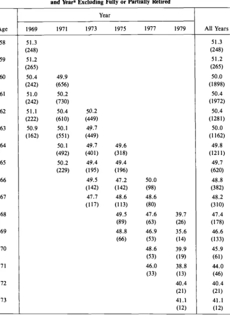
The data in tables 6.5 and 6.6 help to clarify the distinction. Mean hours of work per week by retirement status and age, as well as employment status and sex, are shown in table 6.5. The first two columns of the table pertain to non-self-employed men. Notice that mean hours of work per week decline with age if those who are fully or partially retired are included in the sample. But among those who are not retired, there is virtually no decline between ages 58 and 63 and very little decline thereafter. Thus almost all of the reduction in hours is due to zero or reduced hours of work among those who are retired.4 The same is true for self-employed men and for women. Most of the numbers in table 6.5 represent averages over two or three survey years. The details by year are shown in tables 6 . A . l

through 6.A.6. In addition to little decline in hours worked per week among the nonretired, table 6.A.6 shows that there is also very little decline in weeks worked per year among men who are not self-employed and not retired.

While this empirical fact is not inconsistent with the hazard model specification of retirement, it is at variance with the standard form of the Brownian motion specification that we shall consider subsequently.

6.1.3 Hazard Model Parameter Estimates

The variables used in our analysis are defined as follows:

Social security (SS) payments: The monthly payments a person would receive were he to retire at a given age.

(11)

Table 6.4 Proportion Retired for Non-Self-Employed Males, by Age and Year

Age 58 59 60 61 62 63 64 65 66 67 68 69 70 71 72 73 Year 1969 1971 1973 1975 1977 1979 12.7 (879) 16.0 (1016) 19.1 (1 026) 23.5 (1076) 31.3 (1 029) 40.5 (912) 19.2 (790) 24.0 (924) 37.1 41.9 (935) (725) 45.9 49.6 (978) (841) 50.4 55.8 (959) (864) 72.9 79.3 (834) (878) 84.9 (881) 85.6 (764) 85.3 (632) 89.7 (712) 91.4 (734) 92.2 (743) 94.0 (749) 95 .O (622) All Years 12.7 (879) 16.0 (1016) 19.2 (1816) 23.8 (2ooo) 36.2 (2689) (45.2) (2731) 54.9 (2506) 77.0 (2498) 84.7 (23 18) 88.0 (2290) 90.3 (2 144) 92.2 (2091) 93.8 ( 1444) 94.6 (1300) 94.3 (683) 95.3 (569) Note: The number in parentheses is the number of observations used to calculate the associated mean.

Change in (A) social security payments: The increment to monthly

so-

cial security payments were a person to work for another year and then retire.

Social security wealth: The present discounted value of social security payments were a person to retire at a given age.

(12)

1 0 0 90 80 v 70- .- 60- : Z 50- ;” 40- 2 30- 20 I- a B - -.&-4---- -

+-..*--

- , @.y-/ ~ f-. -

i p

p7

P - J

Jf

d/‘

lY

- /+’ 10- 0 . 4 - 1 1 1 1 1 1 1 1 1 1 1 1 1 1 1 1 1 L 56 58 60 62 64 66 68 70 72

Fig. 6.2 Proportion retired by age and year for non-self-employed males.

Table 6.5 Mean Hours of Work per Week by Age, Sex, Employment Status, and Retirement Status 58 59 60 61 62 63 64 65 66 67 68 69 70 71 72 73 Men Not Self-Employed Not Totala Retired 42.4 42.8 42.3 42.8 41.8 42.2 41.5 42.1 41.0 42.1 40.8 42.4 39.3 41.5 36.5 41.3 33.8 41.2 32.2 39.6 30.0 38.8 29.8 39.4 28.2 37.1 28.9 36.9 25.9 35.6 29.8 36.0 Self-Employed ~~ ~~~ ~ ~ Not Totala Retired 48.7 50.0 47.2 49.6 47.5 49.4 46.7 49.0 45.3 48.8 43 .O 48.2 42.0 49.2 37.7 47.4 37.6 45.6 35.3 46.0 37.0 47.0 32.6 43.5 34.7 47.2 31.9 41.4 31.6 43. I 30.6 35.8 Women Not Totala Retired 38.1 38.5 37.1 38.0 31.3 38.7 36.5 38.2 35.8 38.6 34.1 38.0 33.5 37.8 30.5 36.4 28.5 35.9 26.7 35.2 26.8 34.8 24.8 34.3 25.5 34.9 24.0 29.5 28.1 33.9 21.1 29.9 =Includes fully or partially retired.

(13)

Table 6.6 Mean of Weeks Worked per Year for Non-Self-Employed Men, by Age and Yearn Excluding Fully or Partially Retired

Age 58 59 60 61 62 63 64 65 66 67 68 69 70 71 72 73 ~~ ~~ Year 1969 1971 1973 1975 1977 1979 49.9 (656) 50.2 (730) 50.4 50.2 (610) (449) 50.1 49.7 (551) (449) 50.1 49.7 (492) (401) 50.2 49.4 (229) (195) 49.5 47.7 ( 142) (1 17) All Years 51.3 (248) 51.2 (265) 50.0 (1 898) 50.4 (1 972) 50.4 (1281) 50.0 (1 162) 49.8 (121 1) 49.7 (620) 48.8 (382) 48.2 (310) 47.4 (178) 46.6 (133) 45.9 (61) 44.0 (46) 40.4 (21) (12) 41.1

aFor 1971-79, the variable is one-half the number of weeks worked in the past two years, while the 1969 variable is usual weeks per year. The number in parentheses is the number of

observations used to calculate the associated mean.

Change in social security wealth: The change in the present discounted value of social security payments were a person to work for another year and then retire.

(14)

Bad health: One if the person reported that poor health “limited the kind and amount of work” he could do, zero otherwise.

Earnings: Estimated earnings were the person to work for an additional year.

Liquidassets: Total of liquid assets.

Pension eligibility: One if the person would receive a private pension were he to retire, zero otherwise.

Education: Years of schooling.

Dependents: Number of completely supported children. Age: Years old.

Because of limitations and apparent inaccuracies in reporting nonliquid assets in the RHS that, in particular, make it difficult to compare these assets from one year to the next, we have not used these values in our analysis. After more concerted data cleaning and estimation, we will probably be able to include nonliquid assets in future work.

The results of four alternative specifications are presented in table 6.7.

The first two use social security payments as an explanatory variable, while the next two use social security wealth instead. Liquid assets are used in one

of

each of these groups.

To interpret the parameter estimates it is helpful to consider a case simpler than ours, with the hazard O(t) = exlBl P - I / a . In this case, the time T to retirement is given by E(7) = exp( - XIDl *a), with ln[E(7)] =

- XlBl *a, so that a unit increase in

XI

yields a percentage change in E(7) equal to

-Dl

- a

.

Our model is more complicated, so that this simple result does not hold, but it is still a useful guide to interpretation. To obtain a better idea of the effects of changes in the variables in our model we must present simulation results. We do this after discussing the parameter estimates themselves.

First we find that an increase in monthly social security payments increases the likelihood of retirement after age 62, while larger increments in payments prolong work. The relevant parameters are measured with con- siderable precision. Thus our results appear to confirm the hypothesis of Blinder et al. (1980), although they think of this increment as an addition to the wage. We obtain comparable results when we use social security wealth instead of payments. According to the likelihood values, however, the social security wealth specification appears to fit the data much better than the payments version.

Poor health reduces the age of retirement substantially, by 1%-2% according to our estimates. Its effect is approximately equivalent to an increase of $70 per month in social security payments between the ages of 62

and 64, according to our results. Poor health has a somewhat greater effect than a $10,000 increase in social security wealth between 62 and 64,

based on specifications (3) and (4). Liquid assets also are associated with earlier retirement, but because we have not calculated the annuity value of

(15)

Table 6.7 Hazard Model Parameter Estimates (Standard Errors in Parentheses)

Variable SS payments, age 62-64 SS payments, age 5 65 A SS payments SS wealth, age 62-64 YS wealth, age 5 65 A SS wealth Bad health Earnings (10,OOOs) Liquid assets (10,OOOs) Pension eligibility Education Dependents Age parameter a Standard deviation of v Likelihood value Sample size (100s) (1 0,000s) ,595 (.067) 1.702 (.OW - 1.020 (.148) - - - .394 (.loo) - .474 (.109) - .033 (.076) ( .025) (.078) 2.695 (.165) 1.509 (.067) - .476 - .608 - 3559.9 2000 Specification .594 (.067) I .73 1 (.069) - 1.022 (.150) - - - .407 (.lo) - .567 (.113) .060 (.009) .029 (.076) ( .026) (.079) 2.739 (.170) I .525 - .481 - .608

-

3553.6 2000 (3) - -

-

.598 ( . a 8 1 1.357 (.089) (.611) .699 (.133) (.155) - 8.265 - .I54

-

- .089 - .453 - .558 (.098) ( .029) (.095) 2.807 (.217) 1.970 (.090) -3213.1 2000 (4) -

-

- .603 (.048) 1.386 (.091) (.613) .780 (.133) (.160) .078 (.025) (.099) - .457 (‘030) - ,559 (.096) 2.860 (.223) 1.991 (.091) - 8.244 - .301 - .097 - 3208.5 2000

these assets their effect cannot be directly compared with the effects of social security payments or wealth.

Finally, we see that the more educated tend to retire later. An additional year of education is associated with about a 1.3% increase in the age of retirement. For example, suppose a person with 12 years of education would retire at age 60. We predict that a like person with 16 years of education would retire at age 63, all else equal. People with more dependent children are less likely to retire.

The only anomalous result is the statistically insignificant effect of private pension eligibility. The RHS provides no details of private pension

(16)

plans, and we suspect that the limited information that is available may simply be inadequate to reveal, even in a gross way, the effects of pension availability.

It could be argued that since social security is dependent in large part on earnings, it may in principle be difficult to distinguish their effects. This possibility seems not to be evident in our results. All the relevant parameters have theoretically plausible signs, with currently available assets increasing the likelihood of retirement and monetary rewards to working decreasing the likelihood of retirement.

To give a better idea of the effects of social security on retirement, according to our estimates, we have performed several illustrative simula- tions. All of them begin with our sample of persons who were 60 years old and not retired in 1969. For this group, we first calculate the average probability of being retired by ages 62, 64, and 66. Estimates are obtained using both specifications (2) and (4) from table 6.7. These estimates are shown in the first column of table 6.8.

The next column presents estimates with all of the social security values reduced by amounts reflecting the increases in primary insurance benefits between 1969 and 1975. According to these calculations, if benefits had been maintained at the 1969 level approximately 3% fewer people would have been retired at age 64 (in 1973) and about 5% fewer at age 66 (in

1975).

These figures may be compared with the labor force participation rates shown in the introduction. The labor force participation rates of men 60- 64 fell 9% between 1969 and 1973 and 13.7% between 1969 and 1975. For men over 65, labor force participation fell 14.5% between 1969 and 1973

and 20% between 1969 and 1975. Thus the increase in social security benefits over this period may account for possibly one-third of the decrease, according to our estimates. Our estimates pertain to retirement status, of course, and a substantial number of retired persons are in the labor force.

Table 6.8 Simulated Probabilities of Retirement, by Age, for Selected Changes in Social Security Provision

Current SS Maintained N o SS

Age Law at 1969 Level 62-64 No SS and No ASS

Using SS Wealth (Specification 4)

62 ,288 .288 ,221 .305

64 .496 .48 1 ,320 .418

66 .686 .655 ,613 .655

Using SS Payments (Specification 2)

62 .324 .322 .288 .278

64 .510 .493 .411 .407

(17)

Our estimated effects of social security appear also to be somewhat lower than those of Hurd and Boskin (1981), although their definition of retirement corresponds more closely to labor force participation than ours does. A good deal of the effect they estimate could pertain t o persons who are retired by our definition.

We also simulated the effects of a much grosser change in social security, allowing payments to begin at 65 instead of 62, but for persons 65

and over assuming the benefits that were actually available t o this age group. The results are shown in columns 3 and 4 of tabulation 1 , assuming in the third column that social security wealth (or payments) is zero for persons 62-64 and in the fourth column that the increment as well is set t o zero. This simple procedure probably makes most sense with respect t o payments. According t o this specification, such a scheme would reduce retirement rates at age 64 by about 20% and at 66 by about 8%. Thus these estimates suggest that changes in social security benefit amounts and in particular the age at which they are awarded could have very substantial effects on retirement behavior.

6.2 A Brownian Motion Retirement Process 6.2.1 The Model

The hazard model of retirement ignores one potentially important piece of information. No use of hours worked is made in that specification. We attempt t o utilize this information in an alternative formulation of the retirement process, based on changes in “desired hours” of work. In this specification, changes in desired hours of work occur with changes in health status, social security wealth, age, and the monetary return t o working. The basic idea is that if desired hours decrease to a sufficiently low level, the person chooses to stop working altogether or t o change jobs. Because of fixed costs of working, desired hours do not need to fall to zero for this change in job status t o occur. We use hours worked information by specifying observed retirement status at time t as a function of observed hours as well as other variables at time t - 1.

To begin, we shall think of retirement occurring when hours of work fall below zero. We later relax this assumption. The analysis of a Brow- nian motion process depends on whether it is possible to move back and forth between the retired and non-retired states. If not, the process is said t o be absorbing. For expository purposes, we shall first present the ideas assuming that retirement is not absorbing. Then we shall assume that it is. It is the second version that we estimate. (In practice, typically retirement from a primary job is absorbing, but after retirement, it is possible to move among levels of work status, including zero hours.) Then we shall relax the implications inherent in this specification by considering desired hours of work versus potential hours of work on a primary job. This

(18)

specification is motivated by the evidence in tables 6.5 and 6.6 that suggest little reduction in observed hours of work as one approaches retirement. Finally, we present parameter estimates, which must be considered preliminary at this stage.

If

Retirement Is Not Absorbing

Suppose that the time path of hours worked by an individual who works H(0) = HO hours at some starting age is described by the graph in figure 6.3. The slope u of the solid line represents the “drift” in hours worked as the person ages. The random deviation E from the drift is as-

sumed to follow a Brownian motion (Weiner) process. That is,

Every increment e(t

+ 6)

- f ( t ) is normally distributed with mean zero and variance u2d; and

The increments for every pair of disjoint time intervals are independent.

It is common to refer to H ( t ) as a Brownian motion process with drift u.

The assumptions imply that at any time t , E(t) is normally distributed with mean zero and variance u2t. And because the increments in the process are assumed independent, hours worked at time t

+

d , given H(t ), is a function only of hours worked at time t (and the drift u). Given Ho, the increment by time t is normally distributed with mean ut and variance u2t, that is,

(10)

where in our example u is negative.

tired at age t, given Ho, is simply

H( t)

-

N(H0

+

ut, &),

If retirement means that H I 0, the probability that the person is re-

r

-w0

+

ut)

1

H(0) = Hol = dl 7 -

In other words, this is the probability that at time t the process was at least

Ho lower than it was at time zero, where the expected fall is ut and the variance of the change is a2t.

(19)

Differences in individuals are accounted for by parameterizing the drift

u. In theory, u could depend on

Ho,

as well as other individual attributes like health. Because the values of variables like pension eligibility change with age, presumably the drift u will also change. Thus we propose a piecewise linear drift with kink points that correspond to ages at the time of the surveys. The graph of H(t) might then look something like figure 6.4, where the first survey is at age t i . Now, given that the individual was working H I hours at age ti, the probability

of

retirement at age t2 is

Analogous expressions apply to subsequent age intervals. Note that the age of the first survey varies among individuals.

The simplicity of this analysis results first from the conditioning on initial hours of work and second from the assumption that retirement is not absorbing. In practice, however, retirement from a primary job is probably absorbing for most people; it is typically not possible to return to work on that job. We shall thus develop a specification analogous to the one above, but with retirement assumed to be absorbing. We shall not estimate the model above to describe retirement but shall return to it in subsequent work to describe work “after retirement.” In this case, the assumptions below seem more plausible to us.

If

Retirement Is Absorbing

Again we condition on initial observed hours

NO,

where more generally initial time is when the first of any two consecutive surveys was conduct- ed. Because the density vanishes at zero, the process is no longer normally distributed at period t but obeys the probability density function

(13) pW,t;Ho) =

1

&zexp[- 2a2t 1 ( H

-

Ho - ut)2 1 9 2uHo ( H

+

Ho - ut)2 2o2t - exp

[

-

az-

where the second of the exponentiated terms in the brackets is the result of the “sink” at zero. (See Cox and Miller 1965.)

Again paralleling Cox and Miller, the probability that retirement has occurred at age t , given

HO

and absorption at zero hours, is

(20)

t

H l i )

u3

.-.

Fig. 6.4

This is analogous to the function G(t) in section 6.1. The probability density function corresponding to the time of absorption is then given by

This is the counterpart to the proportional hazard density in equation (2).

The likelihood function for this model is formed from the expression for p ( * ) in equation (13) and G ( . ) in equation (14). That is, the person either is working at level H , with likelihoodp( a ) , or has retired, with probability G . Observations from the first survey are used only to condition the observed outcome at the time of the second survey. (In future work we shall enter an expression for the likelihood of the first-survey outcome.) Persons are followed only through the survey period in which they retired, at which point they are presumed to have been absorbed into the retirement state.

This analysis is based on the implicit assumption that hours of work can be reduced continuously until the person no longer wants to work at all; then retirement occurs. But suppose that the alternative to retirement is working the customary hours on a primary job, as suggested by the sum- mary data presented above. The specification in the next section is intended to address this concern.

If

Desired Hours Diverge from Production Practice

Suppose now that we think of desired hours of work decreasing with age, like actual hours of work in the section above. We use H to indicate desired hours. Suppose that actual observed hours, denoted by

A,

may diverge by an amount d from desired hours. Assume that observed hours be-

fore retirement represent required hours on the primary job. Finally, suppose that an individual retires if desired hours fall below a. These ideas are reflected in figure 6.5.

(21)

Fig. 6.5

The person will retire by t if during this period H(t) falls from

Ho

+

d to a, that is, if the process falls by an amount

(Po

+

6) - a. Of course, we do not observe d or a, only

PO.

To develop the likelihood of this outcome, we shall begin by writing out the probability that the process H ( t ) falls from

H(0) to the level a by t . First we write the probability density function for H a t age t , given the initial position Ho and the absorbing barrier at a, as

d H , t ; H o , a) =

1 H - Ho - ut)*

2u(a

-

Ho)

-

( H

-

No

-

~ ( u - H o )

-

ut)2 2u2t

(16)

1

The probability that retirement has occurred by t is given by G(tlH0,a) =

["-%"'

I

(17) = 1 - 1 - q ) 2u(a - Ho a2 a - HO - ut - ( a

-

Ho)

-

ut

+

exp( 2u(a - Ho cr2

+

exp( a - HO - ut

= 4

6

- ( a

-

Ho)

-

ut

-3

If a = 0, equations (16) and (17) reduce to equations (13) and (14), respectively. Note that G gives the probability that the process falls from Ho to a, sometime before t .

We would like to know the probability that the process falls from

go

+

d to

a.

If we substitute

PO

+

d for HO in equation (17), then the terms a

-

HO in (17) become a - d - = b -

A.

We of course know neither a nor d . Suppose, however, that b varies randomly across individuals. In this in- stance it is natural to assume that b is distributed normally, say with mean vb and variance a;. If this density is denoted by

f,

then the probability of

(22)

retirement for an individual with unknown b is obtained integrating over all values of b, giving

(18)

At least the deviation d = HO -

RO

is likely to depend on age. Thus in principle we should allow shifts in U b with age. The estimates below, how-

ever, allow only for a single b. 6.1.2 Estimates

At its current stage of development the outstanding weakness of the model is that it does not allow for permanent unobserved individual effects. We intend to extend the specification to the case of unobserved individual effects in subsequent work. We give the first set of results in table

6.9. The results in columns 1 and 3 are based on the equations (13) and

(14) in section 6.2 above. Those in columns 2 and 4 are based on the specifications in section 6.3, and allow the absorbing barrier to be estimated. The variable definitions coincide with the definitions used in table 6.7 for the hazard model. The results are considerably easier to interpret than the hazard results because the implicit left-hand variable is desired weekly hours.

In the first column note that the size of social security payments has an important effect on desired hours, with the size of payments after age 65

having a larger effect. But the change in social security payments has a negative sign-indicating that, contrary to expectation, desired hours fall with expected increases from working. The effect is estimated very pre- cisely. The effect on desired hours of work, however, is very small, less than one hour per $100 increase in the payment increment, for example. Earnings have the expected effect, although the size of the effect is again small. Bad health and pension eligibility both have large and significant effects on desired hours. In column 2 we estimate a more general specification by allowing the absorbing barrier to differ from zero as in our second model. The estimate of the barrier is about four hours, which leads to a small decrease in the magnitude of the other coefficient estimates. How-

ever, the relative magnitudes remain constant for the effects of the right- hand-side variables.

In column 3 we replace social security payments and their change with social security wealth measures. The model does not fit the data as well, in contrast to our findings for the hazard model. Neither social security wealth before age 65 nor earnings significantly affects desired hours. Fur- thermore, the change in social security wealth again has the “wrong” sign, although its effect on desired hours is small. The effects of bad health, pension eligibility, and the socioeconomic variables are quite similar to the results for the model with social security payments instead of social security wealth.

(23)

Table 6.9 Brownian Motion Process Parameter Estimates (Standard Errors in Parentbeses) Variable SS payments, age 62-64 SS payments, age L 65 A SS payments (100s) SS wealth, age 62-64 SS wealth, age z 65 A SS wealth (1000s) Bad health Earnings (1000s) Pension eligibility Education Dependents Constant Absorbing barrier Standard deviation Likelihood value Sample size ( 1 ( 1 ooos) - 3.35 - 6.38 (1.77) (1.32) - ,583 (.072) - - - - 8.58 (1.53) .161 (.103) 2.40 (1.40) .660 (.191) .542 (.767) - 13.42 (3.40) - 30.25 (1.01) - 12598.5 2000 Specification -3.15 (1.60) (1.19) - .543 - 5.87 (. 064) -

-

- - 7.68 (1.37) .I39 (.117) - 2.20 (1.27) .592 (.172) .495 (.692) - 11.81 (3.40) 3.96 (.025) 27.44 (.868) - 12387.8 2000 (3) - - - .019 (.065) (.050) (.046) - .306 - .128 - 6.86 (1.51) - .019 (.132) - 3.30 (1.41) .594 (.195) 1.90 (.821) - 20.2 (2.77) - 30.42 (1.09) - 12962.1 2000 (4) - - - .023 (.063) (.048) (.045) (1.432) .03 1 (.127) ( 1.355) 368 (.187) 1.806 (.785) (2.639) 1.982 (.018) - .290 - .125 - 6.574 -3.083 - 19.405 29.08 (1.02) - 2000 6.3 Conclusions

Our results suggest a strong effect of social security benefits on the probability of retirement. Increases in real earnings decrease the likelihood of retirement. Increases in future social security benefits decrease the probability of retirement, according to the results we find the most re- liable. Our major conclusions are based on a hazard model specification of retirement. We also presented a Brownian motion formulation of retirement and presented some initial results based on it. Our hope is that future work will yield a more satisfactory version of the model.

(24)

Notes

1 . Other recent applications of the hazards model are Diamond and Hausman (1982) and

2. From selected issues of Employment and Earnings, table A-4.

3. We standardize by setting the mean of the distribution equal to one. Sensitivity of the results to the distribution assumptions is investigated by Lancaster (1979), Lancaster and Nickell (1980), Baldwin (1983), and Heckman and Singer (1984).

4. See Gustman and Steinmeier (1981) for similar evidence. Flynn and Heckman (1982).

Comment

Gary Burtless

This paper contains a careful assessment of alternative mathematical representations of the retirement process. Contrary to the promise implied by its title, the paper is only tangentially concerned with effects of health and social security on retirement. Its main concern is accurate statistical representation of processes that occur over time. Two representations are considered. The first section contains an analysis using a hazard-rate model. The second contains a novel representation of continuous time processes, which the authors refer to as a “Brownian motion” model.

There are several fundamental problems in modeling the retirement process. Unlike consumption of margarine or housing or trips to Disney- land, there is no natural translation of retirement into a consumption rate per unit of time. One either is or is not retired. And in most cases retirement, like death, is an “absorbing” state: one seldom returns.

This would present no special problems if all the factors affecting retirement were constant, or at least reasonably

so,

before the actual date of retirement. In that case, exogenous variables relevant to estimation would essentially be fixed at the start of the lifetime or working life. The analyst could proceed with estimation exactly as he does in estimating an ordinary demand relationship, with “fraction of expected lifetime devoted to retirement” being the dependent variable instead of consumption of margarine or housing services or whatever.

Of course, there are a couple of special problems. Retirement must be defined, which is not an easy task when some individuals define themselves as retired even though working 40 hours a week, while others persist in saying they’re not retired even though they have not worked full time for years. Another problem is that we do not observe expected lifetimes, nor do we necessarily observe retirement ages for all persons in a cohort. Some respondents have not retired by the last survey date, so their retirement ages are unobserved. Death also interferes with unbiased estimation. If a respondent dies before he retires, the analyst is denied the oppor-

(25)

tunity of observing a retirement age. From the point of view of the analyst-though not of the respondent-this is an inconvenience much like the case of nonretirement.

The problems just mentioned can be surmounted using due care as well as modern statistical models that handle sample censorship. In fact, ex- cept for the now trivial problem of censorship, with sufficiently good observations one could estimate demand for retirement using ordinary least squares.

But the major problem in estimation is the fact that most factors affecting retirement are changing, even as the retirement decision is being made. Someone previously in good health has a heart attack at age 55. Someone steadily employed on a $10-an-hour job is unexpectedly laid off, perhaps permanently. Unanticipated inflation erodes the value of a pension entitlement. These changes alter the economic trade-offs involved in retirement. The margarine consumer can take the price of margarine as well as other relevant factors t o be fixed in making his weekly or monthly pur- chases, and the economist can analyze this consumption behavior accord- ingly. But the case of retirement is much less straightforward.

A common way to get around this problem is to analyze retirement over only a very short period, such as a year. The idea is that the variables affecting retirement are unlikely t o change much over this period, so unanticipated changes can be safely ignored. The obvious problem with this strategy is that the sample of nonretirees at the beginning of some interest- ing year-say age 62-is highly self-selected. It excludes all individuals whose tastes or circumstances caused them t o retire before age 62. So the results cannot be generalized to the whole population without strong untested assumptions. Considering all individuals’ statuses-rather than changes in status-at age 62 causes a different kind of problem. The characteristics that initially caused retirees in this sample t o retire may have changed by age 62, although their retirement status obviously has not. Consequently, the factors inducing retirement are only partially observed.

The contribution of Hausman and Wise is to offer two mathematical formulations of the retirement process that get around these problems. They essentially observe 10 years of individuals’ lives and then try t o model the dynamic process that causes them t o retire before, during, or after that interval.

Their first model is based on the hazard or time-to-failure model first popularized in the biometrics literature, and subsequently applied in so- ciological work on marital separations and in economic research on the duration of unemployment spells. It is assumed that consumers have two choices at any point in time, t o remain at work or to become retired. In any unit of time a certain fraction of individuals will choose to retire. By selecting a convenient mathematical representation of that probability

(26)

density, the authors can easily compute the finite probability that retirement will occur between any two arbitrarily selected points. The method of maximum likelihood estimation finds those parameter values that most closely fit the observed retirement patterns in the sample, including retirees, nonretirees, and the deceased. It is then straightforward to modify this density function to take account of variables such as race and sex that are fixed over time. Essentially these factors have a proportional impact on the probability density, raising or lowering the chance of retirement as the case may be. The authors further modify their specification to permit these variables to have impacts that vary in different time periods-before and after age 65, for example. Individual-specific random differences are also introduced, though I wonder what practical effect this has on the parameter estimates.

To take care of time-varying variables-such as wealth, wages, and social security entitlements-the authors essentially divide up the individual’s lifetime into short time periods-two-year intervals-and then assume that in each period the variable has an effect on retirement probabilities that is proportional to its average value in that period.

The estimates from this model indicate that social security has an extremely modest effect. They show that the 20% increase in real benefit levels in 1972 reduced the fraction of men working at age 64 by 1.5 percentage points, from around half to slightly less than half. It reduced the fraction working at age 66 by about 3 percentage points. These results are very similar to those recently obtained by Robert Moffitt and me (Burtless and Moffitt 1985). In obtaining our results we used the same data set as Hausman and Wise but a substantially different representation of the retirement process.

But the authors are unsatisfied with the economic underpinnings of the hazard rate model, so they go on to estimate a “Brownian motion” model. The idea here is that retirement takes place when an unobserved index of work preferences falls below a critical threshold value. They call this unobserved index “desired hours,” and they assume the index trends downward during advanced age, though it also has random disturbances that may cause it to rise temporarily at certain ages. Estimates from this ingenious model are not very satisfactory, and I find them less easy to interpret because they are expressed in terms of unobserved desired hours rather than in more natural units of measurement, for example, average retirement ages or retirement probabilities per year. The sign of one of the social security coefficients is opposite to the one expected. This coefficient shows, contrary to the earlier result, that as the gain in future social security benefits from extra work rises, nonretirees desire to work fewer hours.

I shall give my reactions to the two models in reverse order. The second model does not seem to me an improvement over the first, so I am not sure

(27)

Table 6 . A . l Mean Hours of Work per Week for Non-Self-Employed Men, by Age

Age 58 59 60 61 62 63 64 65 66 67 68 69 70 71 72 73

-

and Year, Including Fully or Partially Retired

Year 1969 1971 1973 1975 1977 1979 42.4 (794) 42.3 (889) 42.1 (842) (832) 41.3 (723) 41.4 (589) 41.7 41.4 (670) 41.3 (741) 41 .O 40.8 (657) (490) 40.4 40.6 (617) (505) 39.2 39.8 (564) (461) 38.3 35.7 (299) (283) 32.8 (259) 33.0 (202) All Years 42.4 (794) 42.3 (889) 41.8 (1512) 41.5 (1573) 41.0 ( 1870) 40.8 (1711) 39.3 (1 408) 36.5 (877) 33.8 (650) 32.2 (592) 30.0 (478) 29.8 (399) 28.2 (239) 28.9 (198) (100) 29.8 (73) 25.9

Note: The number in parentheses is the number of observations used to calculate the associated mean.

why the authors felt it was needed. They state or imply that the economic rationale for the first model is unconvincing, but they do not show why the second model is better. In a future version of the paper, their reasoning needs to be made clearer.

I do not see why unobserved “desired hours’’ are a better way to model retirement than the simpler on/off representation implicit in the hazard

(28)

Age

Table 6.A.2 Mean Hours of Work per Week for Non-Self-Employed Men, by Age

and Year, Excluding Fully or Partially Retired

~ ~~~ ~ Year 1969 1971 1973 1975 1977 1979 58 59 60 61 62 63 64 65 66 67 68 69 70 71 72 73 42.8 (774) (854) (8 18) 42.4 (789) 42.3 (665) 42.5 (531) 42.8 42.4 41.8 (641) 41.7 (7 12) 42.0 42.1 (597) (441) 42.3 42.2 (542) (444) 41.4 41.5 (482) (395) 42. I 41.4 (222) (192) 41.5 (139) 39.1 (1 15) 40.8 (96) 39.2 (80) 38.5 (63) 38.9 (53) 37.6 (43) (33) 40.1 All Years 42.8 (774) 42.8 (854) 42.2 (1459) 42.1 (1501) 42.1 (1 703) 42.4 (1517) 41.5 (1191) 41.3 (606) 41.2 (377) 39.6 (309) 38.8 39.4 (167) (84) 36.9 (73) 35.6 (35) 36.0 (215) 37.1 (31) Note: The number in parentheses is the number of observations used to calculate the associated mean.

rate model. As the authors’ own statistics on average weekly hours show, there is no tendency for actual (as opposed to desired) hours to decline pri- or to retirement. Why assume that the underlying process causing retirement is any different from the process we typically observe? What we observe is a steady level of work effort until the retirement age, at which point work effort drops significantly.

(29)

Table 6.A.3 Mean Hours of Work per Week for Self-Employed Men, by Age and Year, Including Fully or Partially Retired

Year Age 58 59 60 61 62 63 64 65 66 67 68 69 70 71 72 73 1969 1971 1973 1975 1977 1979 48.7 (167) 47.2 ( 176) ( 159) (172) 45.4 ( 176) 42.7 (172) 46.4 46.4 48.5 (174) (187) 45.8 44.7 (131) (130) 43.2 43.0 (145) (150) 42.6 40.8 (153) (109) 37.7 36.9 (137) (114) 38.6 (94) 35.8 47.0 (103) 42.4 (86) 38.7 (83) 39.7 (72) 33.6 (73) 35.5 (57) 33.2 (68) 34.5 (83) 36.3 (79) (65) (71) 31.8 33.0 (71) (56) 33.9 35.5 (63) (56) (64) (48) (43) 30.6 (45) 40.4 35.2 31.3 32.7 31.0 All Years

Nore: The number in parentheses is the number of observations used to calculate the associated mean.

Their hazard rate model is extremely well implemented and explained, although I think they should go into more detail in explaining their representation of time-varying variables: What are the implications of their particular specification?

(30)

Table 6.A.4 Mean Hours of Work per Week for Self-Employed Men, by Age and Year, Excluding Fully or Partially Retired

Age

-

58 59 60 61 62 63 64 65 66 67 68 69 70 71 72 73 Year 1969 1971 1973 1975 1977 1979 50.0 (147) 49.6 (148) 48.5 (133) 48.5 (145) 48.7 (137) 47.5 (125) 48.9 ( 5 5 ) 48.4 (41) 47.0 (38) 45.4 (25) 44.6 (25) 44.0 (25) 46.7 (28) 46.9 (33) 50.7 44.8 (36) (36) 43.9 42.5 (33) (26) 43.0 52.0 (26) (23) 41.6 41.2 (25) (19) (12) 35.8 (18) 43.1 All Years 50.0 ( 147) 49.6 (148) 49.4 (288) 49.0 (302) 48.8 (334) 48.2 (338) 49.2 (2 19) 47.4 (158) 45.6 (114) 46.0 (99) 47.0 (97) 43.5 (84) (49) (44) 43.1 (12) 35.8 (18) 47.2 41.4

Note: The number in parentheses is the number of observations used to calculate the associated mean.

My final comment should not be taken as a criticism of this work but as a statement of how far we still need to go in this kind of research. The main problem with these models, it seems to me, is that they take full account of a worker’s history but no account of his potential history. For ex-

(31)

Table 6.A.5 Mean Hours of Work per Week for Women, by Age and Year,

Age 58 59 60 61 62 63 64 65 66 67 68 69 70 71 72 73 -

Including Fully or Partially Retired

Year 1969 1971 1973 1975 1917 1979 37.7 (200) 35.5 (220) 35.0 36.1 (216) (137) 34.3 33.6 (193) (155) 35.2 31.5 (194) (165) 31.2 31.3 (139) (114) 32.2 (1 10) 27.8 (76) 33.5 ( 106) 28.3 (84) 24.4 28.4 (96) (60) 26.2 25.9 (79) (53) 28.7 23.6 (77) (53) 27.0 24.3 (56) (46) 26.7 (48) 24.3 (29) 27.4 (46) 22.8 (47) 24.1 (42) 23.7 (31) 28.1 (36) 21.1 (22) All Years

Note: The number in parentheses is the number of observations used to calculate the associated mean.

ample, consider the social security entitlement. The hazard rate model in- tegrates over all past values of potential social security entitlements the worker might have had up t o his observed age at retirement. All potential entitlements he might receive from working one extra year in the future, or two or 10 extra years, are ignored. But of course these potential entitle-

(32)

Table 6.A.6 Mean Hours of Work per Week for Women, by Age and Year,

Excluding Fully or Partially Retired

Age 58 59 - 60 61 62 63 64 65 66 67 68 69 70 71 72 73 _ _ Year 1969 1971 1973 1975 1977 1979 39.2 (180) 37.4 (200) 37.8 39.4 (180) (110) 37.8 37.0 (156) (125) 38.5 36.6 (154) (125) 37.4 37.3 38.3 (76) 35.7 (90) (72) (40) 38.5 (80) 33.8 (56) 30.7 (46) 36.9 (34) 34.9 (45) 38.3 (24) All Years

Note: T h e number in parentheses is the number of observations used to calculate the associated mean.

ments and their rate of change may be exactly the factors motivating the worker when he chooses t o retire. Consider the worker who retires at age

64, perhaps because he was laid off. Why does he not attempt t o find another job? Why does he choose, instead, to retire? Perhaps because the rate of return from added work, in terms of added social security wealth,

(33)

drops sharply at age 65. His decision is motivated by the future drop in social security entitlements rather than by the change he is now experiencing or has experienced in the past.

This is just a special case of the nonlinear budget constraint problem that Hausman and Wise understand very well: Since the price of retirement is not constant, to properly model the consumer’s choice the analyst should include all the relevant prices-including the prices the consumer chooses not to face. By ignoring future retirement prices, the hazard model may misrepresent the retirement process. However, in view of the pro- gress this paper represents over most past models of retirement, this should be considered a relatively minor quibble.

References

Baldwin, R. H. 1983. Army recruit survival functions: Estimation and strategy for use. Ph.D. dissertation, Massachusetts Institute of Tech- nology.

Blinder, A.; Gordon, R.; and Wise, D. E. 1980. Reconsidering the work disincentive effects of social security. National Tax Journal 33:43 1-42.

Boskin, M., and Hurd, M. 1981. The effect of social security on retirement in the early 1970’s. NBER Working Paper no. 659.

Burtless, G., and Moffitt, R. A. 1983. The effect of social security on labor supply of the aged: The joint choice of retirement date and post-retirement hours of work. Mimeographed. Rutgers, N. J.: Rutgers Uni- versity, University of Wisconsin and Mathematical Policy Research.

.

1985. The just choice of retirement age and postretirement hours of work. Journal of LaborEconomics 3 (April).

Cox, D., and Miller, H. D. 1965. The theory of stochasticprocesses. New York: Chapman & Hall.

Diamond, P. A. , and Hausman, J. A. 1982. Individual retirement and savings behavior. Mimeographed. Cambridge: Massachusetts Institute of Technology, Department of Economics.

Flyen, C., and Heckman, J . 1982. New methods for analyzing structural models of labor force dynamics. Journal of Econometrics 18: 115-68.

Gustman, A., and Steinmeier, T. 1984. Partial retirement and the analysis of retirement behavior. Industrial and Labor Relations Review 37~403- 15.

Hausman, J . , and Wise, D. 1978. A conditional probit model for qualitative choice: Discrete decisions recognizing interdependence and hetero- geneous preferences. Econometrica 42; 403 -26.

Heckman, J . , and Singer, B. 1984. The identifiability of the proportional hazard model. Review of Economic Studies.

(34)

Kalbfleisch, J. D., and Prentice, R . L. 1980. The statistical analysis of failure time data. New York: Wiley.

Karlin, S . , and Taylor, H. 1975. Afirst course in stochasticprocess. New York: Academic Press.

Lancaster, T. 1979. Econometric methods for the duration of unemployment. Econornetrica 47 : 939-5 6.

Lancaster, T., and Nickell, S. 1980. The analysis of re-employment probabilities for the unemployed. Journal of the Royal Statistical Society

McFadden, D. 1973. Conditional logit analysis of qualitative choice behavior. In Frontiers in econometrics, ed. D. Zarmbka. New York: Aca- demic Press.

(35)