Do child tax benefits affect the wellbeing of children? evidence from Canadian child benefit expansions

(1)

Do Child Tax Benefits Affect the Wellbeing of

Children? Evidence from Canadian Child Benefit

Expansions

∗

Kevin Milligan

Department of Economics

UBC

and NBER

kevin.milligan@ubc.ca

Mark Stabile

School of Public Policy and Governance, and Rotman School of

Management

University of Toronto

and NBER

mark.stabile@utoronto.ca

The Suntory Centre

Suntory and Toyota International Centres for Economics and Related Disciplines

London School of Economics and Political Science Houghton Street

London WC2A 2AE

PEP 1 Tel: (020) 7955 6674

∗_{This research has been supported by a CLSRN grant. We thank Josh Lewis for excellent}

research assistance. We also thank seminar participants at Alberta, Cornell, Dalhousie, Georgia State, LSE, McGill, RAND, and Simon Fraser, as well as lunch workshop participants at UBC and several conference participants and discussants for many very helpful suggestions. This paper represents the views of the authors and does not necessarily reflect the views of Statistics Canada. The data used in his article can be obtained through application to Statistics Canada’s Research Data Centre program at

(2)

Abstract

A vast literature has examined the impact of family income on the health and development outcomes of children. One channel through which increased income may operate is an improvement in a family’s ability to provide food, shelter, clothing, books, and other expenditure-related inputs to a child’s development. In addition to this channel, many scholars have investigated the relationship between income and the psychological wellbeing of the family. By reducing stress and conflict, more income helps to foster an environment more conducive to healthy child development. In this paper, we exploit changes in child benefits in Canada to study these questions. Importantly, our approach allows us to make stronger causal inferences than has been possible with the existing, mostly correlational, evidence. Using variation in child benefits across province, time, and family type, we study outcomes spanning test scores, mental health, physical health, and deprivation measures. The findings suggest that child benefit programs in Canada had significant positive effects on test scores, as has been featured in the existing literature. However, we also find that several measures of both child and maternal mental health and well-being show marked improvement with higher child benefits. We find strong and interesting differences in the effects of benefits by sex of the child: benefits have stronger effects on educational outcomes and physical health for boys, and on mental health outcomes for girls.

(3)

Public Economics Programme

The Public Economics Programme was established in 2009. It is located within the Suntory and Toyota International Centres for Economics and Related Disciplines (STICERD) at the London School of Economics and Political Science. The programme is directed by Frank Cowell and Henrik Kleven. The Discussion Paper series is available free of charge. To subscribe to the PEP paper series, or for further information on the work of the Programme, please contact our Research Secretary, Leila Alberici on:

Telephone: UK+20 7955 6674 Fax: UK+20 7955 6951 Email: l.alberici@lse.ac.uk

Web site: http://sticerd.lse.ac.uk/PEP

© Authors: Kevin Milligan and Mark Stabile. All rights reserved. Short sections of text, not to exceed two paragraphs, may be quoted without explicit permission provided that full credit, including © notice, is given to the source.

(4)

Introduction

A primary tool for addressing child poverty and increasing the chances for children to succeed in school, and subsequently the labor market, is income transfers to families with children. Almost all developed countries either have direct child benefits or target welfare/social assistance benefits at families with children. These benefits are meant to help achieve several goals. First, by investing in children of lesser means, society aims to provide these children with opportunities to be well-adjusted and productive members of society, with improved educational, and later, labor market outcomes. Second, benefit programs allow society to help achieve distributional and equity goals regardless of the future returns of these transfer programs.

Child benefit programs, as well as social assistance programs that target groups such as single parents with young families, transfer income to expand the budget set of qualifying families. There are several potential mechanisms through which this expansion of family budgets may improve outcomes for children. On the one hand, families may simply use the income to purchase more goods and services, including those goods that are valuable in maintaining basic child welfare and also for enhanced child development (food, clothing, books, etc.). On the other hand, income transfers may have indirect effects such as reducing stress and improving household relations, increasing the chance and opportunities for employment, and others. These indirect channels, while not goods and services purchased with the extra income, may benefit family members, including children, and therefore improve their ability to function, learn, and improve themselves.

(5)

These two channels are explored in Mayer (1997) and Yeung et al (2002), among others, and we borrow terminology from the previous literature here. Direct purchases of resources useful for child development is called the ‘resources’ channel. Improved family relations and emotional well-being is called the ‘family process’ channel. While the majority of the economic literature has focused on the resources channel, our paper instead examines the effects of benefit programs on a wide range of child outcomes which fall naturally under the family process channel. Recent research (Currie and Stabile, 2009; Currie, Stabile, Manivong and Roos, 2008) has documented a strong relationship between early child mental health and not only short term educational achievement, but longer-term economic outcomes such as welfare take-up. So, findings about the impact on children have important long-run implications into adulthood.

The paper offers two main contributions to the previous work in this area. First, it uses an exogenous source of child benefit income based solely on legislative variation rather than the observed income or other choices made by the family. Second, it uses a detailed Canadian survey of child well-being that includes several important outcomes of interest spanning test scores, mental health, physical health, and poverty measures. This survey allows a more rigorous examination of the family process channel than has been explored in previous work.

Our findings suggest that child benefit programs in Canada had significant positive effects on several measures of both child and maternal mental health and well-being, as well as a few measures of child physical health. We also find evidence of direct effects of child benefits on test scores. Interestingly, we find strong differences in the outcomes improved by child benefits by the sex of the child. For boys, benefits have much stronger effects on educational outcomes and physical health measures. For girls, benefits have much stronger effects on mental health measures. These differences suggest that the channels through which benefits improve outcomes may be multiple and may differ by gender.

(6)

Previous work

There is an extensive literature on the broader relationship between income and child health and development.1 Several difficulties make the study of this relationship complex,

including measuring income, distinguishing between permanent or transitory effects, finding exogenous ways to measure income, capturing the effects of other inputs into this production relationship, and finding the proper outcomes to capture the potential effects. Further, documenting a relationship between family income and child outcomes does not in itself help us understand through which channels income works to achieve any measured effects. Mayer (1997) provides a thorough treatment of the sociological theory and developed new empirical evidence based on the NLSY, finding that income was not a strong determinant of long-run outcomes. Blau (1999) presents a discussion of these issues from an economist’s perspective and reviews much of the previous literature that does not deal directly with the issue of the endogeneity of income. Using fixed effects models and the NLSY, Blau concludes that the effects of permanent family income on test scores are small compared to other family and child characteristics, leaving income transfers as a poor policy tool to improve the outcomes of low-income children.

On the other hand, a more recent study by Dahl and Lochner (2008), also using the NLSY, finds reasonably substantial effects of income on child test scores. Dahl and Lochner use changes in the earned income tax credit over several years to exogenously identify income through fixed-effect IV models. This identification strategy relies on federal changes in the benefit structure of the EITC and the tax code over time that has different impacts at different points of the income distribution. Two important contrasts with our work are that we build our

1

(7)

estimates on across-province and across family-size variation and that we incorporate a much broader set of outcomes than just test scores.

A study in the child development literature by Yeung, Linver, and Brooks-Gunn (2002) focuses on understanding the channels through which family income matters for child development. The authors hypothesize and test the two channels discussed earlier in the introduction, being resources and family process. The authors use the Panel Study of Income Dynamics to test these two perspectives. They find stronger evidence in support of the second hypothesis than the first although these results are primarily based on direct OLS estimates of this relationship including a wide variety of explanatory variables. So, while suggestive, it is difficult to draw causal inferences from this evidence. Morris et al. (2004) examine the effects of U.S. welfare reform and antipoverty policies on child wellbeing at different points in the life cycle. Their findings suggest improvements in child wellbeing as a result of policy changes for children making the transition into middle childhood but negative effects of the same set of policies for children making the transition into early adolescence suggesting that similar policies may indeed have very different implications for different children at different times.

In a Canadian study using the National Longitudinal Survey of Children and Youth, Dooley and Stewart (2004) employ a variety of OLS and fixed-effects models to estimate the relationship between family income and test sores. The results from these models are similar to those found in Blau (1999) in that they find a small relationship between income and test scores. They also find some limited impact of the resources channel through measures of children’s activities (day camps, sports, etc.) and housing amenities.

Previous literature has also explored the relationship between shocks to parental socioeconomic status and child wellbeing by examining the effects of job displacement for the father on later life income by the family (Oreopoulos et al., 2005). The findings suggest that

(8)

there are strong intergenerational effects of worker displacement, with children of fathers who were displaced earning less, having higher unemployment and higher take-up of social assistance than otherwise equal children of non-displaced workers.

Our work builds on this literature in a variety of ways. First, we exploit variation over time, across provinces, and across number of children, to develop an exogenous measure of benefit income as an instrument for child benefits. Second, we are able to examine a variety of outcomes, including test scores, but also including a variety of physical and mental health measures. As a result we are able to provide an exogenous estimate of the effects of benefit income on a variety of potential pathways for child development, and on a standard set of test score measures to capture child outcomes.

Policy

The Canadian child benefit system consists of two main benefits. First, the Canada Child Tax Benefit (CCTB) is paid to parents of children age 0 to 17. This is a federal benefit initiated in 1993 that pays the same across the country with two small exceptions.2 The CCTB is payable for

a twelve-month period running from July to June, with the amount dependent upon the reported net income of the parents in the previous calendar year.3 So, the July 2005 to June 2006

maximum annual benefit of $1,228 per child was reduced based on reported family net income from 2004. Benefits do not depend on earned income specifically, so families with no income still qualify for the benefit. Take-up is high—in many provinces the application is given to

2

In Alberta, the benefit is differentiated by age of the child. For example, in 2005 children age zero to six received $1,124 while those age 16 to 17 received $1,423. Until 1997, benefits paid to Quebec residents depended on how many children were in the family, with higher-order children receiving more benefits. We account for each of these exceptions in our benefit calculator.

3

For 2005, the clawback threshold is $36, 378, with a reduction rate of 2.5 percent for income over that threshold for one-child families, and 5 percent for two or more child families.

(9)

families of newborns and the administration is well-integrated with the tax system so any tax filer who qualifies will be made aware of the transfer. The benefit level was constant in nominal dollars between 1993 and 1999, but has been indexed to CPI inflation since 2000. A small supplement ($86 annually in 2005) is available for a third or higher order child, and another supplement ($243 annually in 2005) was available until 2006 for children age zero to six for those not claiming childcare expenses.

The second component of the child benefit system is the National Child Benefit program, begun in 1998. This program is a federal-provincial initiative that features a federally-paid benefit called the National Child Benefit Supplement (NCBS). Provinces, at their discretion, could subtract the NCBS from welfare recipients in their province and use the ‘savings’ to fund different provincial programs and child benefits. This yielded substantial differences in benefits across provinces. In addition, the province of Quebec, while it elected to stay outside the NCB program, instituted major reforms of its child benefits system in 1997 and 2005. The details of each province’s programs are provided in the Appendix. In short, two provinces introduced new transfers that weren’t related to earnings, two provinces introduced earnings-related benefits, and three provinces did both. Across provinces, there were large differences in the structure of benefits across family size.

In addition, some provinces have provincially-funded and administered benefits. In particular, Manitoba and Quebec feature unique components to their system and British Columbia introduced a benefit very similar to the National Child Benefit Supplement two years before the rest of the country in 1996. These elements are also included in our measure of child benefits.

The net impact of these changes is a large degree of heterogeneity in child benefits across several dimensions: year, province, number of children, and income. There is no explicit

(10)

dependence of benefits on marital status or education, but benefit levels across those dimensions will vary through differences in family income. Because our empirical strategy will attempt to exploit only the exogenous components of policy variation, we concentrate primarily on three dimensions of heterogeneity (year, province, number of children).

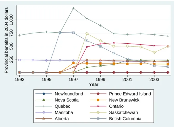
We provide several figures to emphasize the extent of variation in these programs. Figure 1 begins with a depiction of the benefits for which a two-child family from Ontario would be eligible through time. The values come from a tax and benefit simulator.4 Importantly, much of

the increase comes for those at 10,000 and 25,000 of income, through the expansion of the National Child Benefit program and the associated provincial program. This is part of the motivation for our focus on the results for lower education families, as they are more likely to be in the lower income ranges that saw the large increases in benefits through the late 1990s. Figure 2 shows the cross-provincial variation in three panels, representing families with one, two, and three children. For these graphs, we use the actual average provincial benefits among low education families in our sample. The differences across provinces are strong. Quebec follows its own path with a large reform in 1997.5 British Columbia moves early by instituting a benefit in

1996. Most other provinces follow in 1998, but some provinces—such as Prince Edward Island—do not institute a provincial benefit. It is these differences across province, through time, and across family size that we exploit in our empirical strategy described below.

Empirical Strategy

A standard model for estimating the impact of child benefits on a variety of child outcomes in the policy context described above would be as follows:

Outcome_pyki =α₀+α₁X_pyki+α₂BEN_pyki+η_pyki (1)

4

We use the Canadian Tax and Credit Simulator (CTaCS). This is described in Milligan (2007).

5

The appendix shows that the province of Quebec is a major and therefore important source of variation in child benefits. Excluding Quebec from the analysis weakens the results presented below, although a good number of the findings still hold, with slightly larger standard errors. These results are available upon request.

(11)

Where the indexes on the variables represent provinces (p), years (y), number of children (k), and families (i). The vector X contains observable family level characteristics as well as control variables for time and province effects. BEN is a measure of benefit income for a family, either reported or derived based on eligibility criteria.

The crucial empirical challenge for estimating the impact of child benefits on outcomes is that individuals who receive benefit income may be different than other households in both observable and unobservable dimensions. Therefore, a standard regression of outcomes on benefit income may lead to biased estimates. OLS regressions of this type show a strong negative relationship between receipt of, or eligibility for, benefit income and outcomes, even controlling for other income sources and a variety of observable characteristics. To overcome this problem, we employ a solution that extracts plausibly exogenous legislative variation in benefits to remove the bias of unobserved correlates of child outcomes. In particular, we use a simulated benefits approach similar to that in Currie and Gruber (1996) where we use variation in benefit eligibility that is unrelated to individual level characteristics. Variation in benefits comes through changes in benefit generosity over time, across provinces, and across number of children. Specifically, the method involves taking a single random sample of families from a data set with detailed income and benefit data and pushing them through a tax and benefit calculator 400 times—once for each of the ten provinces, each of the ten years between 1994 and 2003, and of four family sizes (0, 1, 2, or 3 children). The tax and benefit calculator we employ is the CTaCS package, which is described in detail in Milligan (2007). The child benefits components of the calculator were developed by looking directly at the legislation and regulations for each province and coding these parameters and program rules into the calculator. We then take the average

(12)

benefit level for each of these cells.6 The resulting benefit levels differ across time periods, years,

and family sizes only through differences in legislated benefit levels and not by income or any unobservables that may be correlated with income. This simulated benefit sample is then used to instrument for actual calculated benefits that a family is eligible for, based on both family and legislative benefit characteristics.

As in Currie and Gruber (1996), we impute the benefit that each family is eligible for by using the family’s income and demographic information available in our data. Reported benefits are available in some years of the data but not all, therefore we rely on calculated benefits based on eligibility and not actual reported benefit data. We explore the relationship between benefits for which families are eligible and true take-up of benefits below to confirm that take-up levels are sufficiently high such that we are capturing the true benefit levels in the population. For the analyses that use sub-samples of the data, such as education group or marital status, we restrict the simulated benefits to the distribution within these sub-samples7.

As described in more detail below, we use the Survey of Labour and Income Dynamics (SLID) to simulate benefits as this survey was designed to collect detailed data on income and benefit eligibility and has far more detailed and accurate income information than the main survey we use to measure child well being, the National Longitudinal Survey of Children and Youth (NLSCY). We aggregate the benefits to the cell level from the SLID and then merge these cells with the NLSCY.

6

From the SLID we take a 10 percent random sample of families with children across all years from 1996 to 2004 This amounts to 9,818 families. The 10% random sample is sufficiently large that there is considerable support across the entire income distribution. For our analysis of sub-samples such as low education, we take the sub-sample of simulated benefits from low-education families to create our cells, not the complete sample. High education families are therefore not included in the simulated cells for low education groups.

7

Specifically, for the entire sample the simulated benefits are collapsed by province, year, and number of children. For the low education sample, the simulated benefits are collapsed by province, year, number of children and education group, and merged back into the individual level data based on the cell groups. Each IV estimate then uses the corresponding benefit cells as the first stage. Using the all-education group set of cells for all first stage

(13)

Using both the individual level imputed benefit, and the simulated aggregate benefit we estimate first-stage equations of the following type:

pyki pyk

pyki

pyki X SIMBEN

BEN =β₀ +β₁ +β₂ +ε . (2)

The imputed child benefit levels BENpyki are predicted by the set of observable characteristics Xpyki and the simulated benefit level SIMBENpyk. We include not only the main effects of

province, years, and number of children, but also the second order interactions of these three factors.

The predicted values from our first-stage can then be used in a second-stage regression using child outcomes, taking the following form:

Outcome_pyki =α₀+α₁X_pyki+α₂B ENˆ _pyki+η_pyki. (3)

The predicted value of the child benefit is used to explain various child outcome measures Outcomepyki. We include the same Xpyki characteristics in the second stage regression

including all second order interactions. In this way, the identification of the impact of child benefits comes through the exclusion of the fully saturated third order interactions of the province, year, and number of children effects. So long as the simulated benefit measure is a good (even if not perfect) predictor of actual benefit eligibility and so long as there are no confounding province-year-number of children trends or policies that invalidate the exclusion restriction, the simulated benefit represents a valid instrument.

ˆ

B EN_pyki

To summarize, our methodology therefore uses 4 steps. 1. We take a random sample of families from the SLID and simulate the benefits these families would be eligible for in each province-year-number of children combination between 1994 and 2004. 2. We aggregate these simulated benefits up to the province-year-number of children cell level and merge these cells into our estimation sample in the NLSCY. 3. We calculate eligible child benefits for each family

(14)

in our estimation sample using all available family characteristics. 4. We instrument for eligible child benefits in the NLSCY using the simulated cells merged from the SLID.

An important challenge to this identification strategy might come from other policy reforms contemporaneous with the changes in child benefits. For example, provincial spending programs introduced as part of the NCB program could have influenced child wellbeing. There were also reforms to provincially-run welfare programs in the mid to late 1990s.8 Similarly, other

policy reforms such as the subsidized childcare program in Quebec studied in Baker, Gruber, and Milligan (2008) might affect the environment. However, our inclusion of province by year effects goes some way to control for most of these concerns. That is, any impact of new provincial spending programs that affects all family sizes equally will be picked up by the province-year dummies as there is no reason to expect them to have differentially impacted families with different numbers of children. The income benefits are the only aspect of policy that explicitly depends on the number of children of which we are aware, however to the extent that other policies have differing impact on families of different sizes our empirical strategy may suffer.

A key assumption underlying this approach is the exogeneity of the province of residence, year, and number of children. For the province, this assumption would be violated if individuals switched provinces in order to benefit from different incentive structures. We consider this possibility unlikely, as the benefits are unlikely to surpass the costs of moving.9 The

number of children may also be influenced by benefits. Assuming that children are exogenous to benefits is standard in the EITC literature in the US (see Hotz and Scholz 2003), but the assumption may be violated if fertility decisions depend on fiscal incentives. Milligan (2005)

8

On both of these points, see Milligan and Stabile (2007) for more policy detail.

9

This claim is supported by recent empirical evidence in Gelbach (2004) who concludes that “ . . . evidence suggests little reason for concern (due to welfare migration) in using cross-state variation in welfare generosity to identify incentive effects of the welfare system on other outcome variables.”

(15)

found strong evidence that fertility did respond to fiscal incentives in Quebec’s Allowance for Newborn Children program in the late 80s and early 90s, but found much less evidence of a response among women more likely to be at-risk for being on welfare.

Data

We use two data sources for the study. Our primary source for data is the National Longitudinal Study of Children and Youth (NLSCY). This survey focuses on Canadian children, with data currently available for six biannual waves spanning 1994-95 to 2004-05. The content of the survey combines extensive parent-reported health, well-being, and developmental information on the child and family with detailed labor market and income information for the parents. The survey initially covered children aged 0 to 11 in wave 1 and has followed that initial cohort to ages 10 to 21 in wave 6. Young children were added in each wave to fill in the gap, allowing cross-sectional coverage of all ages.10

We use all families in each of the NLSCY waves with children ages 10 and under. We focus on children of these ages as the majority of outcomes of interest are asked on a consistent basis to this subset. The resulting data set comprises approximately 56,000 observations over six cycles. However, for many of the outcomes we examine, the variables are limited to explicit age ranges, making the sample sizes for the analysis considerably smaller that the full data set. Finally, because there is some over-sampling of children in smaller provinces, we use the provided weights to recover population-level results.

The NLSCY contains several variables spanning achievement measures, physical, and mental health including having repeated a grade, a math score, a PPVT score, having been diagnosed with a learning disability, measures of hyperactivity, emotional and anxiety disorders,

10

For wave 5, cross-sectional child observations were only added in the age range 0-5. Because the longitudinal cohort was ages 8-19 in wave 5, this left an unfilled gap at ages 6-7 for wave 5. Similarly, there is an age gap in the range 6 to 9 for wave 6.

(16)

physical aggression, suffering from hunger, height and weight, and mother’s health status. Means and age ranges for the variables presented in each of the results tables.

Questions are asked of the person most knowledgeable about the child (in 92% of cases this is the mother) about whether the child repeated a grade in past two years. The Peabody Picture Vocabulary Test is administered to children ages 4-6 and is a widely used measure of cognition for preschoolers. In the NLSCY, mathematics tests were administered to children in grades two through ten (beyond the age limits of our sample) and are based on the Canadian Achievement Tests. Response rates for the Math tests are slightly low and various researchers have investigated how these low response rates might bias analysis using the test scores11 and

have concluded that the low response is random, for the most part. The question on learning disabilities asks about whether the child has been diagnosed and is answered by the person most knowledgeable about the child. The questions on mental and emotional health are asked of parents of all children aged 4 through 11 (we list the questions in the data appendix). The responses to these questions are categorized by disorder, and then added together to determine a hyperactivity score (8 questions), an emotional behavior score (8 questions), an aggressive behavior score (6 questions) an indirect aggression score (5 questions), and a prosocial behavior score (10 questions) for the child. The mother’s depression score is again based on a series of twelve questions asked to the child’s mother about her feelings and behavior over the past week.

The child and mother health questions are reported based on a 5 point scale for self-assessed health of excellent to poor. We combine the bottom three measures for the child as very

11

In cycle 5 the response rate for the mathematics test was 81%. Currie and Stabile (2006) discuss an analysis of the non-responses to the NLSCY math tests for previous cycles performed by Statistics Canada which reports little difference between responders and non-responders at that time. In the cycle 5 codebook, Statistics Canada notes that the response rate is lower in higher grades, and higher among students who performed well on previous cycle math tests.

(17)

few parents report their child to be in poor health. Height and weight measures are also self-reported by the parent as are measures of injuries in the past twelve months, and reports of the child experiencing hunger because of lack of resources to buy food.

Parent reports about their children are sometimes thought less reliable. Parents may hold a more optimistic opinion of their child’s abilities and activities than a disinterested observer. Beyond any bias in their true assessments, parents might also be reluctant to report low achievements out of shame or embarrassment. On the other hand, differences in parent versus expert reports may lie in differences in information—parents may be better informed and thus make more accurate reports. Evidence suggests that parent reports can be reliable in the spheres of motor milestones (Bodnarchuk and Eaton 2004), child health (Spencer and Coe 1996), and behavior and temperament (Clarke-Stewart et al. 2000). However, the validity of the particular measures in the NLSCY may differ from the measures in those studies. A common finding in the literature on validity of parent-reported measures is that the validity of parent-reports for acute events (such as an illness or the reaching of a milestone) is higher than for more general and broad questions.12

The other survey we use is the Survey of Labour and Income Dynamics (SLID), stacking together the public-use cross sections for the years 1996 to 2004. We use this survey both to populate our simulation sample used to generate the simulated child benefits and also for validation of the predictive power of the simulated benefits as the SLID, unlike the NLSCY, has actual reported child benefits for the entire range of years used in our study. The SLID is conducted annually by Statistics Canada with a stratified random sampling of Canadians. With survey weights, the data are potentially nationally representative. The SLID provides detailed information on demographics, and more precise information on income and benefits received

12

Baker, Gruber, and Milligan (2008) have an extensive discussion of the measures in the NLSCY in their Appendix B.

(18)

over the past year than the NLSCY which allows us to provide more complete income and benefit information to the tax calculator. In particular, the income measures available on the SLID are attached from the respondent’s income tax records, which makes them quite relevant for the tax calculator. The sample size per year is around 35 thousand census families made up of 60 thousand individuals aged 15 and higher.

Results

The first set of results we present shows the mean benefit levels federally, provincially, and in total. We next explore the first stage relationship between our simulated child benefits and actual reported child benefits. Following the discussion of the first stage results, we turn to our analysis of child and family outcomes from the NLSCY. Our main specifications use the simulated benefits to instrument for eligible imputed benefits and rely on within province-year-number of children variation as discussed above. We consider the entire sample of children, as well as samples by sex of the child and also present results for children of mothers with lower levels of education, as these families are more likely to be eligible for child benefits (as shown below). We show our analysis in three groups of outcome variables: education, mental and emotional wellbeing, and health and nutrition. Finally, we present specification checks that use alternative sub-samples.13

For all continuous variables, we have normalized the variables using the mean and standard deviation, so that the coefficients can be interpreted in terms of changes in standard

13

The models estimates here all include multiple children from the same household due to the sampling in the NLSCY. We have re-estimated all the models using only a single child from each family and find very similar results with little change in the P-values.

(19)

deviations. The key independent variable is the dollar value of child benefits. All dollar values in the paper are transformed to 2004 constant dollars.

Benefit levels

Table 1 presents the mean and standard deviation of benefit levels at the federal and provincial level, as well as the total. We show the results across all observations and broken down by mother’s education. This is important to understand where our variation is coming from and to motivate our sample choices and robustness checks. The data used for this table is the 2004 SLID for families with a child under or at age 10, with all results in 2004 dollars.

The first row indicates that 85 percent of Canadian families receive some child benefits, with an average amount of $2,174—this includes those with zero in the average. Not shown in the table, a breakdown by income shows that the proportion of families with income under $60,000 receiving some child benefits is almost 1—in the SLID take-up appears close to universal. Only 28.8 percent of families receive any provincial benefits, reflecting both more narrow income targeting and also that several provinces have no provincial benefit. The average benefit is only $222, but among those receiving any benefit it is $769.

The last four rows break down the sample into groups by maternal highest level of education. For high school graduates and drop-outs, over 90 percent are receiving benefits. This reflects low income levels for these families, not an education-related take-up rate. While the proportion receiving benefits remains relatively high across all education groups, the average benefit does decline sharply, reflecting the phase out of benefits at higher income levels. The provincial benefits are positive for only 14.6 percent of families, with a much lower average

(20)

amount. This is important because our identifying variation comes not from province (and family size) level variation. For higher education families, the provincial benefits are not sizeable.

The relationship between simulated benefits and reported child benefits

We begin with an analysis of the relationship between our simulated child benefits and actual reported child benefits in the SLID. This analysis allows us to validate the accuracy of our simulated benefits. These first stage results are performed using the person files of the SLID for the years 1996 to 2004. The SLID includes a much larger sample than the NLSCY, is specifically designed as an income survey, and includes reported benefit information for all of the years in our time span of interest. These three reasons make it a preferable data source for validation of our benefit simulation.

The results appear in Table 2. Each result in the table comes from a separate regression of reported child benefits on simulated benefits with a set of standard control variables. The controls include year dummies, province dummies, number of children dummies, respondent and spouse education and age group dummies, a marital status indicator, and age of youngest child dummies. A standard error, clustered at the province level, is reported beneath in parentheses. The different rows of the table show results from different subsamples of the SLID data. The columns show results using different formulations of the policy variable. The first column shows results using a difference-in-differences specification that exploits only province-year variation. We show the first stage for this more limited source of variation for the purpose of better understanding how much the differences across family size benefit our first stage.In the province-year models, the simulated benefit cells are aggregated at the province-year level (as

(21)

opposed to the province-year-number of kids level as described above) and then merged back with the individual level data. The second column uses a triple-difference specification with simulated benefits varying on a province-year-number of children basis—this is the main specification used in our analysis and includes all two-way interaction terms. The third column is also a triple difference specification, but uses a measure of child benefits that adjusts for the reduction of welfare benefits resulting from the NCB clawback. That is, it accounts for the net change in income.14

The first result is a regression using families with a child age 0 to 17, which captures any families potentially eligible for child benefits. The reported coefficient of 0.941 indicates that an extra $1 of simulated benefits is predicted to increase reported child benefits by $0.941. The result is highly significant and indicates that the simulated benefits are a very precise and accurate predictor of reported child benefits. The coefficient is little-changed in the triple difference specifications in columns two and three. The next row restricts the sample to children age 0 to 10, which is the age range we use for the NLSCY analysis to follow. In this sample, the province-year specification shows an increase in actual benefits of $1.354 for every $1 of simulated benefits. In the second and third columns, the estimated coefficient falls back under $1.00. In the subsample containing only those observations where the respondent has high school education or less, the point estimates in the triple-difference specifications are slightly lower at $0.860 and $0.868, but remain highly significant. As with all of our results here, we cannot reject the hypothesis that the coefficient equals 1.0. Overall, the analysis of the relationship between our simulated benefits and actual child benefits in the SLID allows for firm confidence that the simulated benefits are good predictors of actual benefits.

14

For these simulations, families in the simulation sample who had social assistance income and were in a

‘clawback’ province had their benefit level adjusted to account for the clawback. See Milligan and Stabile (2007) for details on the clawback.

(22)

Effects of Child Benefits on Child Outcomes

We now present the main results that examine the effects of child benefits on three sets of outcomes. These results use the National Longitudinal Survey of Children and Youth, which, as noted above, has detailed measures on educational outcomes, mental/behavioral outcomes, and physical health outcomes. All our results are IV results where the instrument is the simulated benefit measure derived from the SLID, as discussed above. First stages from these results are reported along with the outcome measures. As we discussed earlier, the NLSCY has weaker income information and incomplete child benefit information. For this reason we impute benefits to our NLSCY observations and instrument for these using the simulated benefit measure. The first stage results computed directly in the NLSCY are not as close a fit as those presented in Table 2 above, but remain strong and significant predictors of eligible benefits with coefficients ranging from 0.47 to 0.66.15 We now turn to presenting the results of each set of outcomes in

turn.

Educational Outcomes

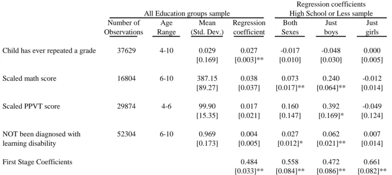
Table 3 contains the results for education outcomes. For each dependent variable, we report the number of observations, the age range covered by the variable, the mean and standard deviation, and finally the coefficient on the benefit variable in four different specifications. The number of observations varies primarily because of differing age ranges for the dependent variables. For example, the PPVT scores are available only for children between ages 4 and 6. Reported are the second stage coefficients on child benefits, using the simulated benefits as an instrument.

15

(23)

The first row reports whether the child has ever repeated a grade. In the full sample, the significant coefficient of 0.027 suggests that an increase of $1,000 in benefits leads to a 2.7 percentage point increase in the probability of having repeated a grade. This result does not persist in the lower education sample including both sexes, and for the lower education sample broken down by sex. This leaves the result inconclusive.

The math and PPVT scores show a small positive, but insignificant, relationship between benefits and test outcomes for the entire sample. However, the results in the low education sample show positive and significant relationships for the math score, and a large but imprecise estimate for the PPVT. For the math score, the coefficient is 0.073, indicating an increase of 7.3 percent of a standard deviation for an increase in $1,000 of benefits. When the lower education sample is broken down by sex we find stark differences. The coefficient for math scores for boys is 0.24 and for the PPVT is 0.392, implying very sizable increases in test scores for boys. In contrast, there is no evidence of an impact for girls.

The final row of Table 3 displays the result for a binary variable describing whether the child has been diagnosed with a learning disability, as answered by the parent. The mean of this variable is 0.969, reflecting the fact that very few children have been diagnosed with a learning disability. The estimated coefficient in the full sample is not statistically distinguishable from zero, but in the high school or less sample the estimated coefficient is a significant 2.7 percentage points. Once again, once the sample is broken down by sex we see that this result is driven by boys with a significant coefficient of 6.2 percentage points, and a small and insignificant coefficient for girls.

Overall, the evidence shows some positive impact on educational outcomes. These results appear to be concentrated among boys of families from lower education households (as measured by the educational status of mother). However, since the full sample includes many

(24)

families who were not recipients of child benefits, we would expect any impact to be diluted. So, the stronger effects in the lower education sample are consistent with expectations. The magnitude of the results is very comparable to other recent work. For example, Dahl and Lochner (2008) find that a $1000 increase in income leads to an increase in math scores of 6% of a standard deviation versus our 7.3% for boys and girls combined.

Mental and Emotional Wellbeing

We now turn to indicators of mental and emotional wellbeing. Recent literature has highlighted the importance of early mental health problems for long-term educational and labour market success (Currie et al, 2008). These dependent variables take the form of scores, aggregated up from responses to individual questions. We report the questions from the questionnaire in the appendix. These scores have been developed in accordance with established practices in developmental psychology. Baker, Gruber, and Milligan (2008) provide some detail on studies of the validity of these measures. For the regressions, we have again scaled the variables by the mean and standard deviation so that coefficients estimates reflect the proportion of a standard deviation resulting from a $1,000 change in benefits.

The first row of Table 4 shows the results for the hyperactivity-inattention score. There is a negative and significant impact in the full sample. In the low education sample, the estimated coefficient is larger in magnitude, but the precision of the estimate is weak, rendering the coefficient insignificantly different from zero. The second row of the table studies the pro-social behavior score. As can be seen in the appendix, these questions reflect how much the child helps other children. The coefficients here are negative, but not significant. For emotional disorder-anxiety, the point estimates are uniformly negative, but not statistically significant anywhere but

(25)

the full sample. Taken together, this evidence is not very informative about the emotional impact of child benefits.

We now turn to measures of aggression. The next row shows the results for conduct disorder-physical aggression, measuring violent acts towards others. The impact with the full sample is negative and statistically significant and is practically identical for the sample from lower education households. When we break down the sample, however, it appears that this result is driven by the girls in the sample. The estimated impact of a thousand dollar increase in child benefits is -0.164, which implies an impact of 16 percent of a standard deviation. The estimated impact on boys is small and insignificant. The table now moves from physical to indirect aggression. Indirect aggression measures social rather than violent conflict with other children. The results here are strongly significant in the low-education sample, and again are driven by a very large result for girls. An extra thousand dollars of benefit is predicted to change girls’ indirect aggression score by 22 percent of a standard deviation.

We close this analysis with an examination of the depression score of the mother. The depression questions are asked of the person most knowledgeable, so to keep the responses consistent we selected only the mothers who were the respondent. The results for this dependent variable are negative and very strong, indicating a significant improvement on maternal depression of increased child benefits. The coefficient on simulated benefits in the full sample is -0.101, which rises to -0.200 in the low-education sample. There are differences in the point estimates for boys and girls, but the confidence intervals overlap.

To summarize, several indicators of emotional and behavioral wellbeing indicate that increased child benefits improve the outcomes of children and their mothers. The results are particularly strong for physical aggression and for maternal depression. Unlike the test score results where it appears that the effects are strongest for the boys from lower education

(26)

households, the effects on mental well-being are concentrated among girls from lower education households in two of the five measures of mental health, and are slightly stronger among the mothers of girls from lower education families for our measure of maternal mental health.

Health and Nutrition

The final set of variables we analyze looks at the health outcomes of children and their mothers. These results are reported in Table 5, following the same format as the previous two tables. In the first row is a dummy variable for never having experienced hunger. The mean of this variable is 0.987, reflecting the fact that very few children in the NLSCY have ever experienced hunger. The results in the full sample show no change in this variable when simulated benefits increase, but in the low education sample the coefficient is 0.014, indicating a small improvement. For hunger, the result is much stronger among boys than girls.

Parent assessments of the child’s general health level show no change in the specifications for both sexes together, but show a negative result for boys only (for this variable, the positive coefficients indicate a worsening of health). For height, there is a fairly large and significant impact on height for low-education boys, but little effect for girls. For weight, there is no significant effect evident. The next row looks at Body Mass Index (BMI) by forming a dummy variable indicating BMI exceeding the age-specific cutoff for obesity. There is a large and significant drop of 6.3 percentage points for boys, but not for girls. For injuries, there is a slight positive impact in the whole sample, but not in the low-education sample.

Overall, the health results show some indication that hunger is reduced, but this appears to have little impact on the general health of the child, although there is some improvement in height but not weight. For the subsample of just boys from lower education household, the effects are much more pronounced with an increase in the number of boys who never experience

(27)

hunger and improved height and lower obesity.16 Again, the results are consistent with other

work in the literature. For example, Anderson et al. (2009) find children ages 2-11 from families at the U.S. poverty line are 2.4 percent heavier than families at three times the poverty line.

Specification Checks:

Tables 6 and 7 present specification checks for our analysis. First, we run seemingly unrelated regression models on the three groups of outcomes: educational, mental and behavioral, and physical health. These models allow us to account for the fact that many of the outcomes in our analysis may be jointly determined. These models are run using the simulated benefit directly in a reduced form version of equation (3) above.17 The results are presented in

Table 6 and focus on the sample of children from low education families. The results from these models are very similar to those presented in Tables 3 through 5 above. We continue to find strong educational effects, particularly for boys. The mental and behavioral effects are also strong (somewhat stronger, in fact, although this is in part due to the reduced form specifications) and the results are, once again, stronger for girls. The physical health effects, on the other hand, are somewhat diminished in these models. Overall, these models suggest that our results are robust to accounting for the possibility that the outcomes examined are jointly determined.

16

Further analysis (not reported here, but available on request) suggests that the height and BMI changes are focused mainly on kids over three years of age. While the change of 14 percent of a standard deviation seems large, it translates into a change of about 1.6 cm or 0.6 inches over the course of the year.

17

In contrast to the models above where we use the simulated benefit to instrument for the imputed benefit level for each family. Using the simulated benefit in the reduced form produces very similar results across all the models estimated. See Milligan and Stabile (2008) for a full set of results using this specification.

(28)

Second, we examine the effects of child benefits on the population least likely to receive benefits and least likely to benefit from the income—children of university graduates. We expect that among this sub-sample, our results should be much weaker. While there still may be examples of university graduates who receive child benefits, the impact should be substantially reduced if we are estimating the true effect of the child benefits on outcomes. Our findings, reported in Table 7, confirm this hypothesis. While we do find a few positive effects of the benefits (on height and physical aggression for example), there are also effects going in the other direction. We interpret this pattern as much weaker than what we observed in the low-education sample, providing us with some additional comfort about our main findings.

Third, in results unreported here we also examined how sensitive our specifications are to the inclusion of separate time trends for each province by number of kids group. For our full sample, (all education groups) this specification yields quite similar results and magnitudes although the standard errors are slightly larger as would be expected. We take this as further evidence that province specific programs outside of the child benefits are not driving our findings. However, for the low-education sample, this specification yields few significant results with standard errors that are considerably larger and it is difficult to make any reasonable inferences here.

Conclusions

In this paper, we study the impact of child benefits on measures of education, emotional and behavioral wellbeing, and health. We find indications that increased child benefits led to improved test scores, decreased aggression and maternal depression, and a reduction in hunger. Our empirical approach based on exogenous policy changes makes us more confident these results are causal than has been possible with the existing, mostly correlational, literature.

(29)

A particularly striking finding in our results is the large difference between the effects of benefit income on boys versus girls. Further, these differences depend on the type of outcome being examined, although they are quite consistent within type of outcome (various health measures versus various education measures). On many of our education and physical health measures we find considerably larger effects for boys. For many of our mental health variables we find considerably larger effects for girls. Finding such differences between sexes is consistent with evidence from other studies examining the impact of various programs on children of various ages (see, for example, Angrist et al (2006), Dynarski (2005) for differences at the college level, and Anderson (2006) for differences at the pre-school level).

Most of the economics research on child benefits has focused on the labor market, educational, and direct-consumption aspects of increased child benefits. We take our findings as evidence that a broader set of outcomes should be included in any assessment of the costs and benefits of expanded transfer payments to families with children.

(30)

References

Anderson, Michael (2006) “Uncovering Gender Differences in the Effects of Early Intervention: A Reevaluation of the Abecedarian, Perry Preschool, and Early Training Projects,” MIT Department of Economics, Ph.D. Thesis.

Anderson, Patricia, Butcher, Kristine, and Diane Whitmore Schanzenbach (2009),

“Childhood Disadvantage and Obesity: Is Nurture Trumping Nature?” in Jonathan Gruber (ed.) The Problems of Disadvantaged Youth: An Economic Perspective. Chicago: University of Chicago Press.

Angrist, Josh, Lang, Daniel, and Phil Oreopoulos (2006), “Lead them to Water and Pay them to Drink: An experiment with services and incentives for college achievement.” NBER Working Paper 12790.

Baker, Michael, Jonathan Gruber, and Kevin Milligan (2008), “Universal Childcare, Maternal Labor Supply, and Family Well-being,” Journal of Political Economy, Vol. 116, No. 4, pp. 709-745.

Blau, David M. (1999), “The effect of income on child development,” The Review of Income and Statistics, Vol. 81, No. 2, pp. 261-276.

Bodnarchuk, J.L. and W.O. Eaton (2004), “Can Parent Reports be Trusted?” Journal of Applied Developmental Psychology, Vol. 25, No. 4,pp. 481-490.

Clarke-Stewart, K.A., Fitzpatrick, M.J., Allhusen, V.D. and Goldberg, W.A., (2000), “Measuring difficult temperament the easy way,”Journal of Developmental and Behavioral Pediatrics, Vol. 21, No. 3, pp. 207–220.

Currie, Janet and Jonathan Gruber (1996), “Health insurance eligibility, utilization of medical care, and child health,” Quarterly Journal of Economics, Vol. 111, No. 2, pp. 431-466.

Currie, Janet and Mark Stabile (2006), “Child Mental Health and Human Capital

Accumulation: The Case of ADHD,” Journal of Health Economics, Vol. 25, No. 6, pp. 1094-1118.

Currie, Janet and Mark Stabile (2009), “Mental Health in Childhood and Human Capital,” in Jonathan Gruber (ed.) An Economic Perspective on the Problems of Disadvantaged Youth. Chicago: University of Chicago Press.

Currie, Janet, Stabile, Mark, Manivong, Phongsack and Leslie L Roos, (2008) “Child Health and Young Adult Outcomes” NBER Working Paper No.

14482.

Dahl, Gordon B. and Lance Lochner.(2008), “The Impact of Family Income on Child

(31)

14,599.

Dooley, Martin and Jennifer Stewart (2004), “Family income and child outcomes in Canada,”

Canadian Journal of Economics, Vol. 37, No. 4, pp. 898-917.

Dynarski, Susan (2005), “Building the Stock of College-Educated Labor,” NBER Working Paper no. 11604.

Gelbach, Jonah (2004), “Migration, the Life Cycle, and State Benefits: How Low is the Bottom?” Journal of Political Economy, Vol. 112, No.5, pp. 1090-1130.

Haveman, Robert and Barbara Wolfe (1995), “The Determinants of Children’s Attainments: A Review of Methods and Findings,” Journal of Economic Literature, Vol. 33, No. 4, pp. 1829-1878.

Hotz, V. Joseph and John Karl Scholz (2003), “The Earned Income Tax Credit,” in Robert Moffitt (ed.) Means-tested Transfer Programs in the United States.Chicago: University of Chicago Press.

Mayer, Susan E. (1997), What Money Can’t Buy. Cambridge MA and London: Harvard University Press.

Milligan, Kevin (2005), “Subsidizing the Stork: New Evidence on Tax Incentives and Fertility,”Review of Economics and Statistics, Vol. 87, No. 3, pp. 539-555. Milligan, Kevin (2007), Canadian Tax and Credit Simulator. Database, software and

documentation, Version 2007-2.

Milligan, Kevin and Mark Stabile (2007), “The integration of child tax credits and welfare: Evidence from the Canadian National Child Benefit program,” Journal of Public Economics, Vol. 91, No. 1-2, pp. 305-326.

Milligan, Kevin and Mark Stabile (2008), “Do Child Tax Benefits Affect the Wellbeing of Children?” NBER Working Paper #14624.

Morris, Pamela, Duncan, Greg, and Elizabeth Clark-Kauffman (2004), “Child Wellbeing in an Era of Welfare Reform: The sensitivity of transitions in development to policy change,” Institute for Policy Research, Northwestern University, Working Paper.

Oreopoulos, Phil, Page, Marianne, and Ann Huff Stevens (2005), “The Intergenerational Effects of Displacement,” NBER Working Paper 11587.

Spencer N.J. and C. Coe (1996), “The development and validation of a measure of parent-reported child health and morbidity: the Warwick Child Health and Morbidity Profile,”

Child: Care, Health and Development, Vol. 22, No. 6, pp. 367-379.

(32)

for Young Children’s Development: Parental Investment and Family Processes,” Child Development, Vol. 73, No. 6, pp. 1861-1879.

(33)

Table 1: Benefit levels by education group

Federal Benefits Provincial benefits Total benefits

Greater Greater Greater

Observations than zero Amount than zero Amount than zero Amount All observations 5134 0.850 2174 0.288 222 0.850 2396

(0.357) (2418) (0.453) (556) (0.357) (2778) High school dropout 484 0.978 3651 0.493 403 0.978 4054

(0.146) (2821) (0.500) (733) (0.146) (3259) High school graduate 763 0.933 2835 0.361 326 0.978 3161

(0.249) (2445) (0.481) (651) (0.249) (2870) Some post-high school 2835 0.884 2199 0.294 211 0.884 2411

(0.320) (2369) (0.456) (527) (0.320) (2710) University degree 1052 0.672 1103 0.146 106 0.672 1209

(0.470) (1756) (0.353) (423) (0.470) (2033)

Notes: Data come from the 2004 SLID.The table shows the proportion of observatios with child benefits greater than zero and the average child benefits (including those with zero). This is repeated for federal benefits, provincial benefits, and total benefits. Beneath each mean is the standard deviation in parentheses. Each row represents a different sample.

(34)

Table 2: The Relationship Between Simulated Benefits and Actual Child Benefits (SLID data)

Nobs. (1) (2) (3)

Type of variation Province- Province-

Province-in policy varible year year-number year-number

children children,

net measure

All kids age 0-17 85396 0.941 0.905 0.884

(0.104) (0.105) (0.102)

Just kids age 0-10 55959 1.354 0.979 0.966

(0.141) (0.135) (0.131)

Kids age 0-10 17704 0.980 0.860 0.868

Just highschool or less (0.260) (0.177) (0.179)

Notes: Regressions using the Survey of Labour and Income Dynamics. Regressors include year dummies, province dummies, respondent and spouse age group dummies, respondent and spouse education group dummies, age of youngest child dummies, and a marital status indicator. The second and third columns also include interaction terms for province*year, year*number of children, and province*number of children.

(35)

Table 3: IV Results: Educational Outcomes

Regression coefficients All Education groups sample High School or Less sample Number of Age Mean Regression Both Just Just Observations Range (Std. Dev.) coefficient Sexes boys girls Child has ever repeated a grade 37629 4-10 0.029 0.027 -0.017 -0.048 0.000

[0.169] [0.003]** [0.010] [0.030] [0.005] Scaled math score 16804 6-10 387.15 0.038 0.073 0.240 -0.012

[89.27] [0.037] [0.017]** [0.064]** [0.014] Scaled PPVT score 29874 4-6 99.90 0.017 0.160 0.392 -0.049

[15.35] [0.021] [0.147] [0.169]* [0.124] NOT been diagnosed with 52304 6-10 0.969 0.004 0.027 0.062 0.007 learning disability [0.173] [0.005] [0.012]* [0.021]** [0.014]

First Stage Coefficients 0.484 0.558 0.472 0.661

[0.033]** [0.084]** [0.086]** [0.082]**

Notes: Data is the NLSCY.Table shows the number of observations, age range, mean, and standard deviation for each dependent variable in the first three columns. The last four columns report coefficients on imputed child benefits for an instrumental variables regression with the indicated variable as the dependent variable. Regressions include province fixed effects, year fixed effects, number of children fixed effects and second order interaction terms between these fixed effects. All regressions also include controls for sex of child, age of child and mother, martial status, mother's education, mother's immigrant status, father's education, father's age, father's immigrant status, urban/rural dummies, Standard errors are clustered at the province level, and reported beneath the estimates, with one star for results significant at the 10 percent level and two stars for those significant at the 1 percent level of significance.

(36)

Table 4: IV Results: Mental and Emotional Wellbeing Outcomes

Regression coefficients All Education groups sample High School or Less sample

Number of Age Mean Regression Both Just Just

Observations Range (Std. Dev.) coefficient Sexes boys girls Hyperactivity-inattention score, 4-11 58916 4-10 4.364 -0.068 -0.121 -0.167 -0.065

[3.373] [0.015]** [0.099] [0.158] [0.045] Prosocial behaviour score - 4-11 42545 4-10 13.068 -0.087 -0.157 -0.157 -0.135 [3.887] [0.057] [0.127] [0.158] [0.109]

Emotional disorder - 58987 4-10 2.426 -0.096 -0.032 -0.031 -0.038

Anxiety score, 4-11 [2.411] [0.023]** [0.033] [0.103] [0.053]

Conduct disorder - physical 58958 4-10 1.421 -0.100 -0.108 -0.044 -0.164

aggression score 4-11 [1.868] [0.032]** [0.055]* [0.080] [0.046]**

Indirect aggression score - 4-11 56634 4-10 0.994 -0.030 -0.156 -0.075 -0.219 [1.562] [0.026] [0.044]** [0.062] [0.026]** Mother's Depression Score 98602 0-10 4.568 -0.101 -0.200 -0.144 -0.221

[5.348] [0.016]** [0.063]** [0.029]** [0.087]*

(37)

Regression coefficients All Education groups sample High School or Less sample

Number of Age Mean Regression Both Just Just

Observations Range (Std. Dev.) coefficient Sexes boys girls Never experienced hunger because o 82134 2-10 0.987 -0.002 0.014 0.036 -0.003

[0.111] [0.003] [0.005]* [0.011]** [0.007] In general, child is in good/fair/poor 108917 0-10 0.118 0.005 0.019 0.050 -0.009 [0.323] [0.003] [0.012] [0.028] [0.007] Current height in metres and centime 91533 0-10 1.086 -0.010 0.045 0.137 -0.012 [0.245] [0.007] [0.025]* [0.048]* [0.015] Current weight of child in kilograms 102424 0-10 21.225 -0.016 -0.038 -0.046 -0.039 [9.752] [0.008] [0.039] [0.040] [0.041]

Obese 67798 0-10 0.199 -0.002 -0.032 -0.063 -0.008

[0.399] [0.004] [0.021] [0.034]* [0.011] injured in last 12 months 108869 0-10 0.094 0.009 -0.004 -0.029 0.011

[0.292] [0.004]* [0.011] [0.023] [0.010] Mother health status is excellent 108065 0-10 0.354 0.011 -0.001 0.022 -0.011 [0.478] [0.009] [0.011] [0.011]* [0.016]

(38)

Table 6: Seemingly Unrelated Regressions Across Outcome Categories

Both Sexes Male Female

Child has ever repeated a grade -0.033 0.012 -0.012

[0.010]** [0.016] [0.011]

Scaled math score 0.067 0.185 -0.024

[0.045] [0.067]** [0.059]

Scaled PPVT score -0.056 0.183 -0.138

[0.077] [0.116] [0.099]

NOT been diagnosed with learning disability 0.036 0.093 0.016

[0.011]** [0.020]** [0.012]

Hyperactivity-inattention score, 4-11 -0.116 -0.174 -0.052

[0.044]** [0.064]** [0.060]

Prosocial behaviour score - 4-11 -0.148 -0.082 -0.201

[0.041]** [0.057] [0.058]**

Emotional disorder - Anxiety score, 4-11 -0.044 -0.076 0.017

[0.044] [0.062] [0.063]

Conduct disorder - physical aggression score -0.128 -0.141 -0.143

[0.042]** [0.065]* [0.054]**

Indirect aggression score -0.088 -0.061 -0.109

[0.050]* [0.063] [0.078]

Mother's Depression Score -0.168 -0.042 -0.267

[0.045]** [0.060] [0.068]**

Never experienced hunger because of lack of money 0.013 0.019 0.006

to buy food. [0.004]** [0.005]** [0.007]

In general, child is in good/fair/poor health -0.005 -0.016 0.005

[0.011] [0.016] [0.015]

Current height in metres and centimetres 0.023 0.041 -0.003

[0.014] [0.020]* [0.021]

Current weight of child in kilograms. -0.031 -0.005 -0.057

[0.019] [0.028] [0.027]*

Obese -0.016 -0.026 -0.002

[0.013] [0.018] [0.019]

Injured in last 12 months 0.008 -0.008 0.018

[0.010] [0.015] [0.013]

Mother health status is excellent 0.003 0.039 -0.022

[0.014] [0.020] [0.020]

Regression Coefficients for High School or Less Sample