On the Number of Planar Orientations with Prescribed Degrees
∗ Stefan Felsner Florian ZickfeldTechnische Universit¨at Berlin, Fachbereich Mathematik Straße des 17. Juni 136, 10623 Berlin, Germany
{felsner,zickfeld}@math.tu-berlin.de
Abstract
We deal with the asymptotic enumeration of combinatorial structures on planar maps. Prominent instances of such problems are the enumeration of spanning trees, bipartite perfect matchings, and ice models. The notion of orientations with out-degrees prescribed by a function α: V → N unifies many different combinatorial structures, including the
afore mentioned. We call these orientations α-orientations. The main focus of this pa-per are bounds for the maximum number of α-orientations that a planar map with n
vertices can have, for different instances of α. We give examples of triangulations with 2.37n
Schnyder woods, 3-connected planar maps with 3.209n
Schnyder woods and inner triangulations with 2.91n
bipolar orientations. These lower bounds are accompanied by upper bounds of 3.56n
, 8n
and 3.97n
respectively. We also show that for any planar map
M and anyαthe number ofα-orientations is bounded from above by 3.73n
and describe a family of maps which have at least 2.598n
α-orientations.
AMS Math Subject Classification: 05A16, 05C20, 05C30
1
Introduction
A planar mapis a planar graph together with a crossing-free drawing in the plane. Many dif-ferent structures on planar maps have attracted the attention of researchers. Among them are spanning trees, bipartite perfect matchings (or more generally bipartite f-factors), Eulerian orientations, Schnyder woods, bipolar orientations and 2-orientations of quadrangulations. The concept of orientations with prescribed out-degrees is a quite general one. Remarkably, all the above structures can be encoded as orientations with prescribed out-degrees. Let a planar mapM with vertex setV and a functionα:V →Nbe given. An orientationXof the
edges of M is anα-orientation if every vertexv has out-degreeα(v). For the sake of brevity, we refer to orientations with prescribed out-degrees simply as α-orientations in this paper.
For some of the above mentioned structures it is not obvious how to encode them as α -orientations. For Schnyder woods on triangulations the encoding by 3-orientations goes back to de Fraysseix and de Mendez [10]. For bipolar orientations an encoding was proposed by Woods [40] and independently by Tamassia and Tollis [35]. Bipolar orientations of M are one of the structures which cannot be encoded as α-orientations on M, an auxiliary map M′ (the angle graph of M) has to be used instead. For Schnyder woods on 3-connected ∗The conference version of this paper is to appear in the proceedings of WG’07 (LNCS) under the title ”On the Number ofα-Orientations”.
planar maps as well as bipartitef-factors and spanning trees Felsner [14] describes encodings as α-orientations. He also proves that the set of α-orientations of a planar map M can always be endowed with the structure of a distributive lattice. This structure on the set of α-orientations found applications in drawing algorithms in [4], [17], and for enumeration and random sampling of graphs in [19].
Given the existence of a combinatorial structure on a class Mn of planar maps with n
vertices, one of the questions of interest is how many such structures there are for a given mapM ∈ Mn. Especially, one is interested in the minimum and maximum that this number
attains on the maps fromMn. This question has been treated quite successfully for spanning
trees and bipartite perfect matchings. For spanning trees the Kirchhoff Matrix Tree Theorem allows to bound the maximum number of spanning trees of a planar graph with n vertices between 5.02nand 5.34n, see [31, 28]. Pfaffian orientations can be used to efficiently calculate the number of bipartite perfect matchings in the planar case, see for example [24]. Kasteleyn has shown, that the k×ℓsquare grid has asymptoticallye0.29·kℓ ≈1.34kℓ perfect matchings. The number of Eulerian orientations is studied in statistical physics under the name of ice models, see [2] for an overview. In particular Lieb [22] has shown that the square grid on the torus has asymptotically (8√3/9)kℓ≈1.53kℓ Eulerian orientations and Baxter [1] has worked out the asymptotics for the triangular grid on the torus as (3√3/2)kℓ≈2.598kℓ.
In many cases it is relatively easy to see which maps in a classMncarry a unique object of
a certain type, while the question about the maximum number is rather intricate. Therefore, we focus on finding the asymptotics for the maximum number of α-orientations that a map from Mn can carry. The next table gives an overview of the results of this paper for different
instances of Mn andα. The entrycin the “Upper Bound” column is to be read asO(cn), in
the “Lower Bound” column as Ω(cn) and for the “≈c” entries the asymptotics are known.
Graph class and orientation type Lower bound Upper bound
α-orientations on planar maps 2.598 3.73
Eulerian orientations 2.598 3.73
Schnyder woods on triangulations 2.37 3.56
Schnyder woods on the square grid ≈3.209
Schnyder woods on 3-connected planar maps 3.209 8
2-orientations on quadrangulations 1.53 1.91
bipolar orientations on stacked triangulations ≈2
bipolar orientations on outerplanar maps ≈1.618
bipolar orientations on the square grid 2.18 2.62
bipolar orientations on planar maps 2.91 3.97
The paper is organized as follows. In Section 2 we treat the most general case, whereMn
is the class of all planar maps with nvertices andα can be any integer valued function. We prove an upper bound which applies for every map and everyα. In Section 2.3 we deal with Eulerian orientations. In Section 3.1 we consider Schnyder woods on plane triangulations and in Section 3.2 the more general case of Schnyder woods on 3-connected planar maps. We split the treatment of Schnyder woods because the more direct encoding of Schnyder woods on triangulations as α-orientations yields stronger bounds. In Section 3.2 we also discuss
the asymptotic number of Schnyder woods on the square grid. Section 4 is dedicated to 2-orientations of quadrangulations. In Section 5, we study bipolar orientations on the square grid, stacked triangulations, outerplanar maps and planar maps. The upper bound for planar maps relies on a new encoding of bipolar orientations of inner triangulations. In Section 6.1 we discuss the complexity of counting α-orientations. In Section 6.2 we show how counting α-orientations can be reduced to counting (not necessarily planar) bipartite perfect matchings and the consequences of this connection are discussed as well. We conclude with some open problems.
2
Counting
α
-Orientations
A planar map M is a simple planar graph G together with a fixed crossing-free embedding planar map
ofG in the Euclidean plane. In particular,M has a designated outer (unbounded) face. We denote the sets of vertices, edges and faces of a given planar map byV,E, and F, and their respective cardinalities by n,m and f. The degree of a vertex v will be denoted byd(v).
Let M be a planar map and α : V → N. An orientation X of the edges of M is an
α-orientationif for all v∈V exactlyα(v) edges are directed away fromv inX. α
-orientation
Let X be an α-orientation of M and let C be a directed cycle in X. Define XC as the orientation obtained from X by reversing all edges of C. Since the reversal of a directed cycle does not affect out-degrees the orientation XC is also anα-orientation of M. The plane
embedding of M allows us to classify a directed simple cycle as clockwise (cw-cycle) if the cw-cycle
interior, Int(C), is to the right of C or as counterclockwise (ccw-cycle) if Int(C) is to the left ccw-cycle of C. IfC is a ccw-cycle ofX then we say thatXC isleft ofXand X isright ofXC. Felsner left of
right of
proved the following theorem in [14].
Theorem 1 LetM be a planar map andα :V →N. The set ofα-orientations ofM endowed
with the transitive closure of the ‘left of ’ relation is a distributive lattice.
The following observation is easy, but useful. Let M and α :V →N be given, W ⊂V and
EW the edges of M with one endpoint in W and the other endpoint in V \W. Suppose all
edges of EW are directed away from W in some α-orientation X0 of M. The demand ofW
for Pw∈Wα(w) outgoing edges forces all edges in EW to be directed away fromW in every
α-orientation of M. Such an edge with the same direction in every α-orientation is a rigid
edge. rigid edge
We denote the number of α-orientations of M by rα(M). Let M be a family of pairs
(M, α) of a planar map and an out-degree function. Most of this paper is concerned with lower and upper bounds for max(M,α)∈MrαM(M) for some familyM. In Section 2.1, we deal
with bounds which apply to allM andα, while later sections will be concerned with special instances.
2.1 An Upper Bound for the Number α-Orientations
A trivial upper bound for the number ofα-orientations onM is 2mas any edge can be directed
in two ways. The following easy but useful lemma improves the trivial bound.
Lemma 1 LetM be a planar map, A⊂E a cycle free subset of edges ofM, andαa function
α :V → N. Then, there are at most 2m−|A| α-orientations of M. Furthermore, M has less
Proof. LetX be an arbitrary but fixed orientation out of the 2m−|A|orientations of the edges
of E\A. It suffices to show that X can be extended to an α-orientation of M in at most one way. We proceed by induction on |A|. The base case |A|= 0 is trivial. If|A|>0, then, as A is cycle free, there is a vertexv, which is incident to exactly one edge e∈ A. If v has out-degreeα(v) respectivelyα(v)−1 inX, thenemust be directed towards respectively away from v. In either case the direction of e is determined by X, and by induction there is at most one way to extend the resulting orientation of E \(A−e) to an α-orientation of M. If v does not have out-degree α(v) or α(v)−1 in X, then there is no extension of X to an α-orientation of M. The bound 2m−n+1 <4n follows by choosing A to be a spanning forest
and applying Euler’s formula.
A better upper bound for generalM and α will be given in Proposition 1. The following lemma is needed for the proof.
Lemma 2 LetM be a planar map withnvertices that has an independent setI2 ofn2 vertices
which have degree 2 inM. Then, M has at most(3n−6)−(n2−1) edges.
Proof. Consider a triangulationT extendingM and letB be the set of additional edges, i.e.,
of edges ofT which are not inM. Ifn= 3 the conclusion of the lemma is true and we may thus assumen >3 for the rest of the proof. Hence, there are no vertices of degree 2 inT, and every vertex ofI2 must be incident to at least one edge fromB. If there is a vertexv∈I2, which is
incident to exactly one edge fromB, thenvand its incident edges can be deleted fromI2, from
M and fromT, whereby the result follows by induction. The last case is that all vertices ofI2
have at least two incident edges inB. Since every edge inB is incident to at most two vertices fromI2 it follows that|I2| ≤ |B|. Therefore,|EM|=|ET| − |B| ≤ |ET| − |I2|= (3n−6)−n2.
Remark. It can be seen from the above proof, that K2,n2 plus the edge between the two vertices of degreen2 is the unique graph to which onlyn2−1 edges can be added. For every
other graph at leastn2 edges can be added.
Proposition 1 Let M be a planar map, α :V → N, and I =I1∪I2 an independent set of
M, where I2 is the subset of degree 2 vertices in I. Then, M has at most
22n−4−|I2|· Y v∈I1 1 2d(v)−1 d(v) α(v) (1) α-orientations.
Proof. We may assume that M is connected. Let Mi, for i= 1, . . . c, be the components of
M −I. We claim thatM has at most (3n−6)−(c−1)−(|I2| −1) edges. Note, that every
component C of M −I must be connected to some other component C′ via a vertex v ∈ I such that the edgesvw and vw′ with w ∈C and w′ ∈ C′ form an angle at v. As w and w′ are in different connected components the edgeww′ is not in M and we can add it without destroying planarity. We can add at leastc−1 edges not incident toI in this fashion. Thus, by Lemma 2 we have thatm+ (c−1)≤3n−6−(I2−1).
LetS′ be a spanning forest ofM −I, and let S be obtained from S′ by adding one edge incident to every v∈ I. Then, S is a forest with n−c edges. By Lemma 1 M has at most 2m−|S|α-orientations and by Lemma 2
For every vertexv∈I1 there are 2d(v)−1 possible orientations of the edges ofM−S atv.
Only the orientations withα(v) orα(v)−1 outgoing edges atvcan potentially be completed to an α-orientation ofM. SinceI1 is an independent set it follows thatM has at most
2m−|S|· Y v∈I1 1 2d(v)−1 d(v)−1 α(v) + d(v)−1 α(v)−1 ≤22n−4−|I2|· Y v∈I1 1 2d(v)−1 d(v) α(v) (2) α-orientations.
Corollary 1 Let M be a planar map and α : V → N. Then, M has at most 3.73n α
-orientations.
Proof. Since M is planar the Four Color Theorem implies, that it has an independent set I
of size|I| ≥n/4. LetI1,I2 be as above. Note, that for d(v)≥3
1 2d(v)−1 d(v) α(v) ≤ 1 2d(v)−1 d(v) ⌊d(v)/2⌋ ≤ 34. (3)
Thus, the result follows from Proposition 1, as 22n−4−|I2| 3 4 |I1| ≤22n−4 3 4 n 4 ≤3.73n.
Remark. The best lower bound for general α and M, which we can prove, comes from Eulerian orientations of the triangular grid, see Section 2.3.
2.2 Grid Graphs
Enumeration and counting of different combinatorial structures on grid graphs have received a lot of attention in the literature, see e.g. [2, 7, 22]. In Section 2.3 we present a family of graphs that have asymptotically at least 2.598n Eulerian orientations. This family is closely related to the grid graph, and throughout the paper we will use different relatives of the grid graph to obtain lower bounds. We collect the definitions of these related families here.
The grid graph Gk,ℓwith krows and ℓcolumns is defined as follows. The vertex set is
Vk,ℓ={(i, j)|1≤i≤k, 1≤j ≤ℓ}.
The edge set Ek,ℓ=Ek,ℓH ∪Ek,ℓV consists of horizontal edges
Ek,ℓH =n{(i, j),(i, j+ 1)} |1≤i≤k, 1≤j ≤ℓ−1o and vertical edges
EVk,ℓ=n{(i, j),(i+ 1, j)} |1≤i≤k−1, 1≤j≤ℓo.
We denote the ith vertex row by ViR = {(i, j) | 1 ≤ j ≤ ℓ} and the jth vertex column by VjC ={(i, j) |1 ≤i≤k}. The jth edge column EjC is defined as EjC ={{(i, j),(i, j+ 1)} | 1≤i≤k}. The number of bipolar orientations ofGk,ℓ is studied in Section 5.1.
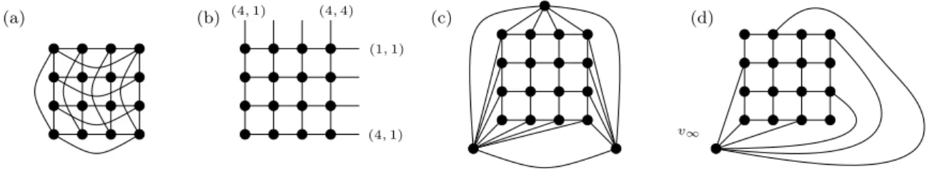
The grid on the torus GT
k,ℓ is obtained from Gk+1,ℓ+1 by identifying (1, i) and (k+ 1, i)
as well as (j,1) and (j, ℓ+ 1) for all i and j, see Figures 1 (a) and (b). Edges of the form {(i,1),(i, ℓ)} are called horizontal wrap-around edges while those of the form {(1, j),(k, j)} are the vertical wrap-around edges. Note thatGk,ℓcan be obtained fromGTk,ℓby deleting the
khorizontal and theℓvertical wrap-around edges.
Lieb [22] shows thatGTk,ℓhas asymptotically (8√3/9)kℓEulerian orientations. His analysis involves the calculation of the dominant eigenvalue of a so-called transfer matrix, see also Section 4. v∞ (1,1) (4,1) (4,1) (4,4) (a) (b) (c) (d)
Figure 1: Two illustrations ofGT
4,4, the augmented gridG∗4,4, and the quadrangulationG4,4.
We consider the number of Schnyder woods on the augmented grid G∗k,ℓ in Section 3.2, see Figure 1 (c). The augmented grid is obtained fromGk,ℓby adding a triangle with vertices
{a1, a2, a3} to the outer face. The triangle is connected to the boundary vertices of the grid
as follows. The vertex a1 is adjacent to all vertices of V1R, a2 is adjacent the vertices from
VℓC and a3 to the vertices fromVkR∪V1C.
When we consider 2-orientations in Section 4 we use the quadrangulation G
k,ℓ, see
Fig-ure 1 (d). It is obtained from the gridGk,ℓ by adding one vertexv∞ to the outer face which is adjacent to every other vertex of the boundary such that (1,1) is not adjacent to v∞. For kand ℓeven this graph is closely related to the torus grid GT
k,ℓ, which can be obtained from
G
k,ℓ by reassigning end vertices of edge as follows.
{(1, j), v∞} → {(1, j),(k, j)} 2≤j≤ℓ {(k, j), v∞} → {(k, j),(1, j)} 2≤j≤ℓ
{(i,1), v∞} → {(i,1),(i, ℓ)} 2≤i≤k {(i, ℓ), v∞} → {(i, ℓ),(i,1)} 2≤i≤k Sincek, ℓare even this does not create parallel edges and the resulting graph isGT
k,ℓminus
the edgese1 ={(1,1),(1, ℓ)}and e2 ={(1,1),(k,1)}.
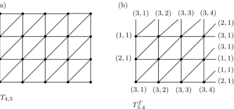
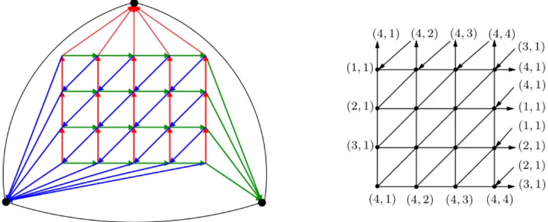
We also use the triangular grid Tk,ℓ in Sections 2.3 and 5.2. It is obtained from Gk,ℓ
by adding the diagonal edges {(i, j),(i−1, j+ 1)} for 2 ≤ i ≤ k and 1 ≤ j ≤ ℓ−1, see Figure 2 (a). The augmented triangular grid T∗
k,ℓ, which we need in Section 3.1 is obtained
in the same way fromG∗k,ℓ, see Figure 7.
The terms vertex row, vertex column and edge column are used for the triangular grid analogously to the definition above forGk,ℓ.
We also use the triangular grid on the torusTk,ℓT , see Figure 2 (b). We adopt the definition from [1], therefore it differs slightly from that of the square grid on the torus. More precisely, instead of identifying vertices (i, ℓ+ 1) and (i,1) we identify vertices (i, ℓ+ 1) and (i−1,1) (and (1, ℓ+ 1) with (k,1)) to obtainTk,ℓT fromTk,ℓ. This boundary condition is called helical.
The wrap-around edges are defined analogously to the square grid case.
Baxter [1] was able to determine the exponential growth factor of Eulerian orientations of Tk,ℓT as k, ℓ → ∞. Baxter’s analysis uses similar techniques as Lieb’s [22] and yields an asymptotic growth rate of (3√3/2)kℓ.
(b) TT 3,4 (3,1) (3,2) (3,3) (3,4) (2,1) (1,1) (1,1) (3,1) (3,1) (3,1) (3,2) (3,3) (3,4) (2,1) (1,1) (2,1) (a) T4,5
Figure 2: The triangular gridT4,5, and T3,4T .
2.3 A Lower Bound Using Eulerian Orientations
Let M be a planar map such that every v ∈ V has even degree and let α be defined as α(v) = d(v)/2, ∀v ∈ V. The corresponding α-orientations of M are known as Eulerian
orientations. Eulerian orientations are exactly the orientations which maximize the binomial Eulerian orientations
coefficients in equation (1). The lower bound in the next theorem is the best lower bound we have for max(M,α)∈MrαM(M), where Mis the set of all planar maps and no restrictions are
made forα.
Theorem 2 Let Mn denote the set of all planar maps with n vertices and E(M) the set of
Eulerian orientations ofM ∈ Mn. Then, forn big enough,
2.59n≤(3√3/2)kℓ≤ max
M∈Mn|E
(M)| ≤3.73n.
Proof. The upper bound is the one from Corollary 1. For the lower bound consider the
trian-gular torus gridTT
k,ℓ. As mentioned above Baxter [1] was able to determine the exponential
growth factor of Eulerian orientations ofTT
k,ℓask, ℓ→ ∞. Baxter’s analysis uses eigenvector
calculations and yields an asymptotic growth rate of (3√3/2)kℓ. This graph can be made into a planar map Tk,ℓ+ by introducing a new vertexv∞ which is incident to all the wrap-around edges. This way all crossings between wrap-around edges can be substituted by v∞. As every Eulerian orientation of Tk,ℓT yields a Eulerian orientation ofTk,ℓ+ this graph has at least (3√3/2)kℓ≥2.598kℓ Eulerian orientations fork, ℓ big enough.
3
Counting Schnyder Woods
Schnyder woods for triangulations have been introduced as a tool for graph drawing and graph dimension theory in [32, 33]. Schnyder woods for 3-connected planar maps are introduced in [12]. Here we review the definition of Schnyder woods and explain how they are encoded as α-orientations. For a comprehensive introduction see e.g. [13].
LetM be a planar map with three verticesa1, a2, a3 occurring in clockwise order on the
outer face of M. A suspension Mσ of M is obtained by attaching a half-edge that reaches
into the outer face to each of these special vertices. special
vertices
LetMσ be a suspended 3-connected planar map. ASchnyder wood rooted ata
1, a2, a3 is
an orientation and coloring of the edges of Mσ with the colors 1,2,3 satisfying the following
rules.
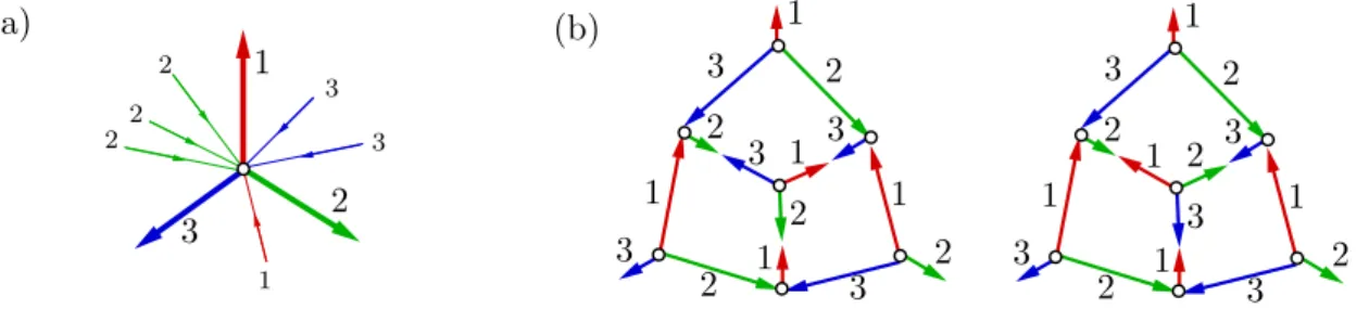
(W1) Every edge eis oriented in one direction or in two opposite directions. The directions of edges are colored such that ifeis bidirected the two directions have distinct colors. (W2) The half-edge at ai is directed outwards and has colori.
(W3) Every vertexv has out-degree one in each color. The edgese1, e2, e3 leavingvin colors
1,2,3 occur in clockwise order. Each edge enteringv in color ienters v in the clockwise sector fromei+1 toei−1, see Figure 3 (a).
(W4) There is no interior face the boundary of which is a monochromatic directed cycle.
2 3 3 2 2 2 1 3 1 (b) (a) 2 1 1 3 1 2 2 1 3 1 2 3 3 2 3 2 1 3 1 2 2 1 3 1 1 3 3 2 3 2
Figure 3: The left part shows edge orientations and edge colors at a vertex, the right part two different Schnyder woods with the same underlying orientation.
In the context of this paper the choice of the suspension vertices is not important and we refer to the Schnyder wood of a planar map, without specifying the suspension explicitly.
Let Mσ be a planar map with a Schnyder wood. Let Ti denote the digraph induced by
the directed edges of color i. Every inner vertex has out-degree one inTi and in fact Ti is a
directed spanning tree ofM with rootai.
In a Schnyder wood on a triangulation only the three outer edges are bidirected. This is because the three spanning trees have to cover all 3n−6 edges of the triangulation and the edges of the outer triangle must be bidirected because of the rule of vertices. Theorem 3 says, that the edge orientations together with the colors of the special vertices are sufficient to encode a Schnyder wood on a triangulation, the edge colors can be deduced, for a proof see [10].
Theorem 3 LetT be a plane triangulation, with verticesa1, a2, a3 occuring in clockwise order
on the outer face. Let αT(v) := 3 if v is an internal vertex and αT(ai) := 0 for i= 1,2,3.
Then, there is a bijection between the Schnyder woods of T and the αT-orientations of the
inner edges ofT.
In the sequel we refer to anαT-orientation simply as a 3-orientation. Schnyder woods on
3-connected planar maps are in general not uniquely determined by the edge orientations, see Figure 3 (b). Nevertheless, there is a bijection between the Schnyder woods of a 3-connected planar mapM and certainα-orientations on a related planar mapMf, see [14].
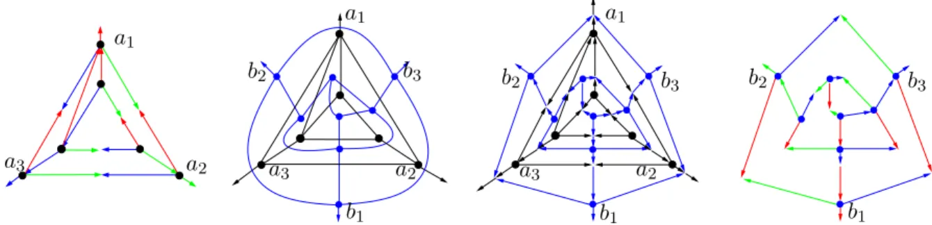
In order to describe the bijection precisely, we first define thesuspension dualMσ∗ofMσ, suspension
dual
which is obtained from the dualM∗ofM as follows. Replace the vertexv∗
∞, which represents the unbounded face ofM inM∗, by a triangle on three new verticesb1, b2, b3. Let Pi be the
those on Pi are incident to bi instead of v∞∗ . Adding a ray to each of the bi yieldsMσ∗. An
example is given in Figure 4.
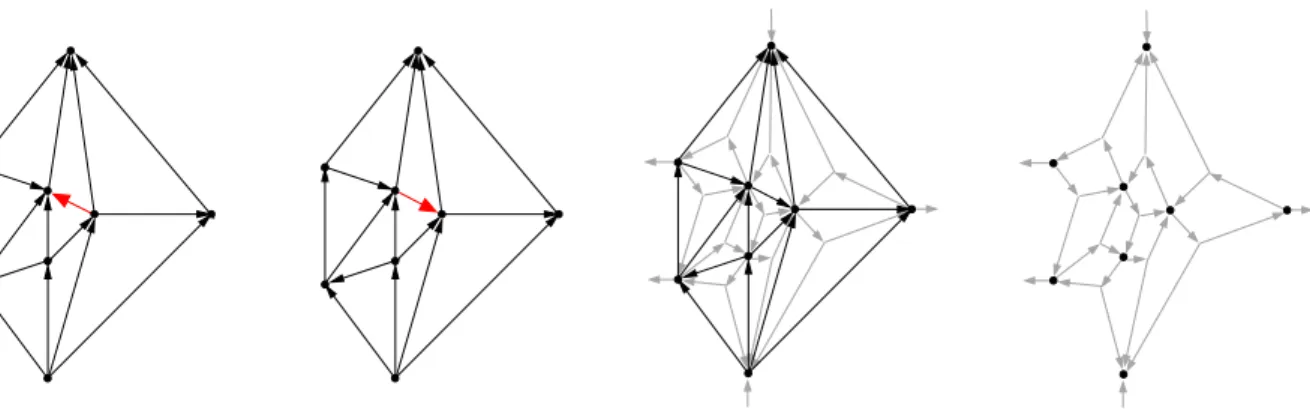
a2 a3 b2 b3 a1 a1 a2 a3 a3 a1 b3 b2 a2 b3 b2 b1 b1 b1
Figure 4: A Schnyder wood, the primal and the dual graph, the oriented primal dual com-pletion and the dual Schnyder wood.
Proposition 2 LetMσ be a suspended planar map. There is a bijection between the Schnyder woods of Mσ and the Schnyder woods of the suspension dual Mσ∗. Figure 5 illustrates how
the coloring and orientation of a pair of a primal and a dual edge are related.
2 3 1 2 1 3 3 2 1
Figure 5: The three possible oriented colorings of a pair of a primal and a dual edge. The completion Mf of Mσ and Mσ∗ is obtained by superimposing the two graphs such
that exactly the primal dual pairs of edges cross, see Figure 4. In the completion Mf the common subdivision of each crossing pair of edges is replaced by a new edge-vertex. Note that the rays emanating from the three special vertices of Mσ cross the three edges of the triangle induced by b1, b2, b3 and thus produce edge vertices. The six rays emanating into the
unbounded face of the completion end at a new vertexv∞ placed in this unbounded face. A pair of corresponding Schnyder woods onMσ and Mσ∗ induces an orientation ofMfwhich is
an αS-orientation where
αS(v) =
3 for primal and dual vertices 1 for edge vertices
0 forv∞.
Note, that a pair of a primal and a dual edge always consists of a unidirected and a bidirected edge, which explains why αS(ve) = 1 is the right choice. Theorem 4 says, that the edge
orientations of Mf are sufficient to encode a Schnyder wood of Mσ, the edge colors can be deduced, for a proof see [14].
Theorem 4 The Schnyder woods of a suspended planar map Mσ are in bijection with the
αS-orientations of Mf.
In the rest of this section we give asymptotic bounds for the maximum number of Schnyder woods on planar triangulations and 3-connected planar maps. We treat these two classes
separately because the more direct bijection from Theorem 3 allows us to obtain a better upper bound for Schnyder woods on triangulations than for the general case. We also have a better lower bound for the general case of Schnyder woods on 3-connected planar maps than for the restriction to triangulations.
Stacked triangulations are plane triangulations which can be obtained from a triangle Stacked tri-angulations
by iteratively adding vertices of degree 3 into bounded faces. The stacked triangulations are exactly the plane triangulations which have a unique Schnyder wood and we have a generalization of this well-known result for general 3-connected planar maps, which we state here without a proof.
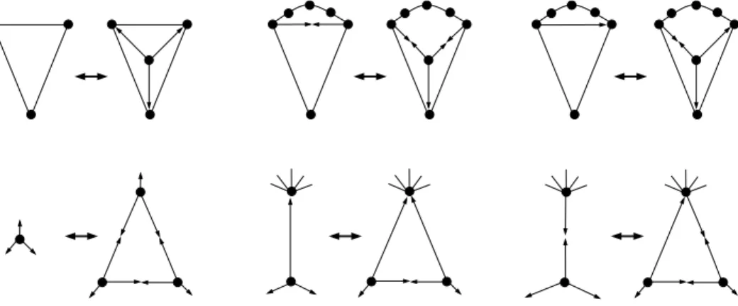
Theorem 5 All 3-connected planar maps, which have a unique Schnyder wood, can be con-structed from the unique Schnyder wood on the triangle by the six operations show in Figure 6 read from left to right.
Figure 6: Using the three primal operations in the first row and their duals in the second row every graph with a unique Schnyder wood can be constructed.
3.1 Schnyder Woods on Triangulations
Bonichon [3] found a bijection between Schnyder woods on triangulations withnvertices and pairs of non-crossing Dyck-paths, which implies that there areCn+2Cn−Cn+12 Schnyder woods
on triangulations withnvertices. ByCnwe denote thenth Catalan numberCn= 2nn/(n+1).
Hence, asymptotically there are about 16nSchnyder woods on triangulations withnvertices. Tutte’s classic result [38] yields that there are asymptotically about 9.48nplane triangulations
on n vertices. See [27] for a proof of Tutte’s formula using Schnyder woods. The two results together imply that a triangulation with n vertices has on average about 1.68n Schnyder woods. The next theorem is concerned with the maximum number of Schnyder woods on a fixed triangulation.
Theorem 6 Let Tn denote the set of all plane triangulations with n vertices and S(T) the
set of Schnyder woods ofT ∈ Tn. Then,
2.37n≤max
T∈Tn|S
The upper bound follows from Proposition 1 by using that for d(v)≥3 d(v) 3 ·21−d(v)≤ 5 8.
For the proof of the lower bound we use the augmented triangular gridT∗
k,ℓ. Figure 7 shows
a canonical Schnyder wood onTk,ℓ∗ in which the vertical edges are directed up, the horizontal edges to the right and diagonal ones left-down.
(4,1) (4,1) (3,1) (1,1) (1,1) (2,1) (2,1) (3,1) (4,2) (4,3) (4,4) (4,1) (4,2) (4,3) (4,4) (3,1) (2,1) (1,1) (4,1)
Figure 7: The graphsT4,5∗ with a canonical Schnyder wood andT4,4 with the additional edges
simulating Baxter’s boundary conditions.
Instead of working with the 3-orientations of T∗
k,ℓ we useα∗-orientations of Tk,ℓ where
α∗(i, j) = 3 if 2≤i≤k−1 and 2≤i≤ℓ−1 1 if (i, j)∈ {(1,1),(1, ℓ),(k, ℓ)} 2 otherwise.
For the sake of simplicity, we refer toα∗-orientations ofTk,ℓ as 3-orientations.
Intuitively,Tk,ℓ promises to be a good candidate for a lower bound because the canonical
orientation shown in Figure 7 on the left has many directed cycles. We formalize this intuition in the next proposition, which we restrict to the casek=ℓonly to make the notation easier.
Proposition 3 The graphT∗
k,k has at least 25/4(k−1)
2
Schnyder woods. For kbig enoughT∗
k,k
has
2.37k2+3 ≤ |S(Tk,k∗ )| ≤2.599k2+3
Proof. The face boundaries of the triangles ofTk,k can be partitioned into two classes C and C′ of directed cycles, such that each class has cardinality (k−1)2 and no two cycles from the
same class share an edge. Thus, a cycleC∈ C′ shares an edge with three cycles from C if it does not share an edge with the outer face ofTk,k and otherwise it shares an edge with one
or two cycles fromC.
For any subset D ofC reversing all the cycles inDyields a 3-orientation of Tk,k, and we
can encode this orientation as a 0-1-sequence of length (k−1)2. After performing the flips of a given 0-1-sequence a, an inner cycle C′ ∈ C′ is directed if and only if either all or none of the three cycles sharing an edge withC′ have been reversed. IfC′ ∈ C′ is a boundary cycle,
then it is directed if and only none of the adjacent cycles from Chas been reversed. Thus the number of different cycle flip sequences on C ∪ C′ is bounded from below by
X
a∈{0,1}(k−1)2
2PC′∈C′XC′(a).
HereXC′(a) is an indicator function which takes value 1 ifC′is directed after performing the flips of aand 0 otherwise.
We now assume that everya∈ {0,1}(k−1)2
is chosen uniformly at random. The expected value of the above function is then
E[2PXC′] = 1
2(k−1)2
X
a∈{0,1}(k−1)2
2PC′∈C′XC′(a).
Jensen’s inequality E[ϕ(X)] ≥ ϕ(E[X]) holds for a random variable X and a convex
functionϕ. Using this we derive that
E[2PXC′]
≥2E[PXC′]= 2PP[C′flippable].
The probability thatC′ is flippable is at least 1/4. ForC′ which does not include a boundary edge the probability depends only on the three cycles fromC that share an edge withC′ and two out of the eight flip vectors for these three cycles makeC′ flippable. A similar reasoning applies forC′ including a boundary edge. Altogether this yields that
X
a∈{0,1}(k−1)2
2PC′∈C′XC′(a)
≥2(k−1)2 ·2(k−1)2/4.
Different cycle flip sequences yield different Schnyder woods. The orientation of an edge is easily determined. The edge direction is reversed with respect to the canonical orientation if and only if exactly one of the two cycles on which it lies has been flipped. We can tell a flip sequence apart from its complement by looking at the boundary edges.
For the upper bound we use Baxter’s result for Eulerian orientations on the torus Tk,ℓT (see Sections 2.2 and 2.3). Every 3-orientation ofTk,ℓ plus the wrap-around edges, oriented
as shown in Figure 7 on the right, yields a Eulerian orientation ofTT
k,ℓ. We deduce that Tk,ℓ∗
has at most 2.599n Schnyder woods.
Remark. Let us briefly come back to the number of Eulerian orientations of Tk,ℓT , which was mentioned in Sections 2.2 and 2.3 and in the above proof. There are only 22(k+ℓ)−1 different orientations of the wrap-around edges. By the pigeon hole principle there is an orientation of these edges which can be extended to a Eulerian orientation ofTT
k,ℓ in
asymp-totically (3√3/2)kℓways. Thus, there are out-degree functionsαkℓforTk,ℓsuch that there are
asymptotically 2.598kℓ α
kℓ-orientations. Note, however, that directing all the wrap-around
edges away from the vertex to which they are attached in Figure 7 induces a unique Eulerian orientation ofTk,ℓ.
We have not been able to specify orientations of the wrap-around edges, which allow to conclude thatTk,ℓhas (3
√
3/2)kℓ3-orientations with these boundary conditions. In particular we have no proof that Baxter’s result also gives a lower bound for the number of 3-orientations.
3.2 Schnyder Woods on the Grid and 3-Connected Planar Maps
In this section we discuss bounds on the number of Schnyder woods on 3-connected pla-nar maps. The lower bound comes from the grid. The upper bound for this case is much larger than the one for triangulations. This is due to the encoding of Schnyder woods by 3-orientations on the primal dual completion graph, which has more vertices. We summarize the results of this section in the following theorem.
Theorem 7 Let M3n be the set of 3-connected planar maps withnvertices andS(M) denote the set of Schnyder woods of M ∈ M3
n. Then,
3.209n≤ max
M∈M3
n
|S(M)| ≤8n. The example used for the lower bound is the square gridGk,ℓ.
Theorem 8 Fork, ℓbig enough the number of Schnyder woods of the augmented grid G∗k,ℓis asymptotically |S(G∗k,ℓ)| ≈3.209kℓ.
Proof. The graph induced by the non-rigid edges in the primal dual completion Ge∗
k,ℓ of G∗k,ℓ
is G2k−1,2ℓ−1 −(2k−1,1). This is a square grid of roughly twice the size as the original
and with the lower left corner removed. The rigid edges can be identified using the fact that αS(v∞) = 0 and deleting them induces α′S on G2k−1,2ℓ−1 −(2k−1,1). The new αS′ only
differs from αS for vertices, which are incident to an outgoing rigid edge, and it turns out,
that α′S(v) = d(v)−1 for all primal or dual vertices and αS′ (v) = 1 for all edge vertices of G2k−1,2ℓ−1 −(2k−1,1). Thus, a bijection between α′S-orientations and perfect matchings
of G2k−1,2k−ℓ−(2k−1,1) is established by identifying matching edges with edges directed
away from edge vertices. The closed form expression for the number of perfect matchings of G2k−1,2k−ℓ−(2k−1,1) is known (see [21]) to be k Y i=1 ℓ Y j=1 4−2 cosπi k −2 cos πj ℓ .
The number of perfect matchings ofG2k−1,2ℓ−1−(2k−1,1) is sandwiched between that
ofG2k−2,2ℓ−2 and that of G2k,2ℓ. Therefore the asymptotic behavior is the same and in [24],
the limit of the number of perfect matchings ofG2k,2ℓ, denoted as Φ(2k,2ℓ), is calculated to
be lim k,ℓ→∞ log Φ(2k,2ℓ) 2k·2ℓ = log 2 2 + 1 4π2 Z π 0 Z π 0
log(cos2(x) + cos2(y))dxdy ≈0.29. This implies that G∗
k,ℓ has asymptoticallye4·0.29·kℓ≈3.209kℓ Schnyder woods.
Remark. In [36] Temperley discovered a bijection between spanning trees ofGk,ℓand perfect
matchings of G2k−1,2ℓ−1 −(2k−1,1). Thus, Schnyder woods of G∗k,ℓ are in bijection with
spanning trees ofGk,ℓ, see Figure 8. This bijection can be read off directly from the Schnyder
wood: the unidirected edges not incident to a special vertex form exactly the related spanning tree. Encoding both, the Schnyder woods and the spanning trees, asα-orientations also gives an immediate proof of this bijection.
We now turn to the proof of the upper bound stated in Theorem 7. The proof uses the upper bound for Schnyder woods on plane triangulations, see Theorem 6. We define a
Figure 8: A Schnyder wood on G∗4,4, the reduced primal dual completion G7,7−(7,1) with
the corresponding orientation and the associated spanning tree.
triangulation TM such that there is in injective mapping of the Schnyder woods ofM to the
Schnyder woods ofTM. The triangulation TM is obtained from M by adding a vertexvF to
every face F of M with |F| ≥4, see Figure 9. The generic structure of a bounded face of a Schnyder wood is shown on the left in the top row of Figure 9, for a proof see [13]. The three
edges, which do not lie on the boundary of the triangle, are thespecial edgesofF. special edges
3 3 1 3 2 3 2 1 3 1 2 3 2 1 3 2 2 2 3 2 3 1 2 1 2 1 2 3 1 2 2 3 1 1 2 3 1 1 1 2 2 1 3 2 1 2 3 3 2 3 2 2 3 1 1 2 1 2 2 3 3
Figure 9: A Schnyder wood on a mapM induces a Schnyder wood onTM. The three special
edges of a face are those, which do not lie on the black triangle.
A vertex vF is adjacent to all the vertices of F. A Schnyder wood of M can be mapped
to a Schnyder wood of TM using the generic structure of the bounded faces as shown in
Figure 9. The green-blue non-special edges ofF become green unidirected. Their blue parts are substituted by unidirected blue edges pointing from their original start-vertex towards vF. Similarly the blue-red non-special edges become blue unidirected and the red-green ones
red unidirected. Three of the edges incident tovF are still undirected at this point. They are
directed away fromvF and colored in accordance with (W3).
Let two different Schnyder woods be given that have different directions or colors on an edgee. That the map is injective can be verified by comparing the edges on the boundary of the two triangles on which the edgeelies in TM.
Thus, it suffices to bound the number of Schnyder woods ofTM. We do this by specializing
Proposition 1. We denote the set of vertices of TM that correspond to faces of size 4 inM
by F4 and its size byf4 and similarlyF≥5 andf≥5 are defined. Note that I =F4∪F≥5 is an
independent set and TM has a spanning tree in which all the vertices fromI are leaves. Let
nT denote the number of vertices ofTM. Then, TM has at most
23nT−6−nT ·Y v∈I 1 2d(v)−1 d(v) 3 ≤4n+f4+f≥5 · 1 2 f4 · 5 8 f≥5 = 4n·2f4· 5 2 f≥5 (4) Schnyder woods. Note that n+f4+f≥5+f4+ 2f≥5≤m+f4+ 2f≥5 ≤3n−6 which implies
that f4+32f≥5≤n. Maximizing equation (4) under this condition yields that the maximum
8n is attained whenf4 =n. ThusM has no more than 8n Schnyder woods.
The proof of the lower bound 3.209ninvolves the result about the number of perfect match-ings of the square grid. This result makes use of non-combinatorial methods. Therefore, we complement this bound with a result for another graph family, which uses a straight-forward analysis, but still yields that these graphs have more Schnyder woods than the triangular grid, see Section 3.1.
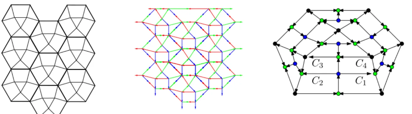
The graph we consider is thefilled hexagonal gridHk,ℓ, see Figure 10. Neglecting bound- filled
hexagonal grid
ary effects he hexagonal grid has twice as many vertices as hexagons. This can be seen by associating with every hexagon the vertices of its northwestern edge. Thus, neglecting bound-ary effects, the filled hexagonal grid has five vertices per hexagon. The boundbound-ary effects will not hurt our analysis becauseHk,ℓ has only 2(k+ℓ) boundary vertices but 5·kℓ+ 2(k+l)
vertices in total.
Proposition 4 Fork, ℓ big enough the filled hexagonal grid Hk,ℓ has
2.63n≤ |S(Hk,ℓ)| ≤6.07n.
C2 C1
C4
C3
Figure 10: The filled hexagonal grid H3,3, a Schnyder wood on this grid and the primal-dual
suspension of a hexagonal building block ofHk,ℓ. Primal vertices are black, face vertices blue
and edge vertices green.
Proof. We count how many different orientations we can have on a filled hexagon. We do
this using the bijection from Theorem 4. The right part of Figure 10 shows a feasible αS
-orientation of a filled hexagon. Note that this -orientation is feasible on the boundary when we glue together the filled hexagons to a gridHk,ℓ and add a triangle of three special vertices
hexagon. As these edges belong to a triangle in the hexagon on their other side, the cycle flips in any two filled hexagons can be performed independently.
Let us now count how many orientations a filled hexagon admits, see the right part of Figure 10 for the definition of the cycles C1, C2, C3 and C4. If the 6-cycle induced by the
central triangle is directed as shown in the rightmost part of Figure 10 then we can flip either C1 or C2 and if C2 is flipped, C3 can be flipped as well. This yields 43 orientations, as the
situation is the same at the other two 4-faces of the hexagon. If the 6-cycle is flipped the same calculation can be done with C3 replaced by C4. This makes a total of 2·43 = 128
orientations per filled hexagon. That is, there are at least 128k·ℓ ≥2.6395·k·ℓ orientations of Hk,ℓ.
We start the proof of the upper bound by collecting some statistics about Hk,ℓ. As
mentioned above, Hk,ℓ has n= 5·k·ℓ interior vertices, 12·kℓedges and 7·kℓ faces. Thus,
the primal-dual completion has 48·kℓ edges. There is no choice for the orientation of the edges incident to the 3·4/7·f = 12·kℓface vertices of triangles. We can choose a spanning tree T on the remaining 5·kℓ+ 12·kℓ+ 3·kℓ vertices such that all face vertices are leafs and proceed as in the proof of Proposition 1, but using that we know the number of edges exactly. Since in the independent set of the remaining face vertices all of them have degree 4 and required out-degree 3, they contribute a factor of 1/2 each. Thus, there are at most 2(48−12−20)k·ℓ·2−3·kℓ= 213·kℓ≤6.07nSchnyder woods on H
k,ℓ.
4
Counting 2-Orientations
Felsner et al. [16] present a theory of 2-orientations of plane quadrangulations, which shows many similarities with the theories of Schnyder woods for triangulations. A quadrangulation is a planar map such that all faces have cardinality four. A2-orientation of a quadrangulation
2-orientation of a quad-rangulation Qis an orientation of the edges such that all vertices but two non-adjacent ones on the outer
face have out-degree 2.
In [15] it is shown that 2-orientations on quadrangulations withn inner quadrangles are counted by the Baxter-numberBn+1. Hence asymptotically there are about 8n2-orientations
on quadrangulations with n vertices. Tutte gave an explicit formula for rooted quadrangu-lations. A bijective proof of Tutte’s formula is contained in the thesis of Fusy [18]. The formula implies that asymptotically there are about 6.75n quadrangulations on n vertices.
The two results together yield that a quadrangulation with n vertices has on average about 1.19n 2-orientations.
We now give a lower bound for the number of 2-orientations of G
k,ℓ. The proof method
via transfer matrices and eigenvalue estimates comes from Calkin and Wilf [7]. There it is used for asymptotic enumeration of independent sets of the grid graph. LetZ(Q) denote the set of all 2-orientations of a quadrangulationQ, with fixed sinks.
Proposition 5 Fork, ℓ big enough G
k,ℓ has
1.537kℓ ≤ |Z(Gk,ℓ)| ≤(8·√3/9)kℓ≤1.5397kℓ.
Proof. We consider 2-orientations of G
k,ℓ with sinks (1,1) and v∞. These 2-orientations induce Eulerian orientations of GT
k,ℓ. The wrap-around edges inherit the direction of the
e1
e2
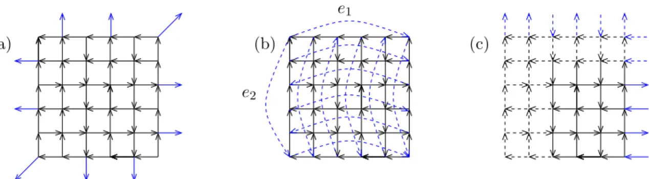
(a) (b) (c)
Figure 11: A 2-orientation of G6,6, the corresponding Eulerian orientationX of GT6,6 and an alternating orientation of GT
4,4 that can be extended to X.
Therefore Gk,ℓ has at most as many 2-orientations as GT
k,ℓ has Eulerian orientations, which
implies the claimed upper bound.
Conversely a Eulerian orientation of GTk,ℓ in which the wrap-around edges have these prescribed orientations induces a 2-orientation of Gk,ℓ. Such Eulerian orientations are called almost alternating orientations in the sequel, see Figure 11 (b).
Proving a lower bound for the number of almost alternating Eulerian orientations yields a lower bound for the number of 2-orientations ofGk,ℓ.
For the sake of simplicity we will work with alternating orientations of GTk−2,ℓ−2 instead of almost alternating ones ofGTk,ℓ. In these Eulerian orientations the wrap-around edges are directed alternatingly up and down respectively left and right, see Figure 11 (c). It is easy to see that this is a lower bound for the number of almost alternating orientations ofGTk,ℓ. Since we are interested in an asymptotic lower bound there is no difference in counting alternating orientations of GT
k−2,ℓ−2 and GTk,ℓ from our point of view and we will continue working with
alternating orientations ofGTk,ℓ to keep then notation simple.
Consider a vertex columnVjC ofGTk,ℓand the edge columnsEjC−1 andEjC. LetX1, X2 be
orientations ofEjC−1 respectively EjC. Let δ(X1, X2) = 1 if and only if the edges induced by
VC
j can be oriented such that all the vertices of VjC have out-degree 2. Let δU(X1, X2) = 1
respectivelyδD(X1, X2) = 1 if and only ifδ(X1, X2) = 1 and the wrap-around edge induced
byVj is directed upwards respectively downwards. Note that
δU(X1, X1) = 1 =δD(X1, X1)
and
δU(X1, X2) = 1⇐⇒δD(X2, X1) = 1.
We define two transfer matricesTU(2k) and TD(2k). These are square 0-1-matrices with
the rows and columns indexed by the 2kkorientations of an edge column of size 2k, that havek edges directed to the right. The transfer matrices are defined by (TU(2k))X1,X2 =δU(X1, X2) and (TD(2k))X1,X2 =δD(X1, X2). HenceTU(2k) =TD(2k)T and T2k=TU(2k)·TD(2k) is a real symmetric non-negative matrix with positive diagonal entries. From the combinatorial interpretation it can be seen thatT2k is primitive, that is there is an integerℓ≥1 such that
all entries ofT2kℓ are positive and thus the Perron-Frobenius Theorem can be applied. Hence, T2k has a unique eigenvalue Λ2k with largest absolute value, its eigenspace is 1-dimensional
LetXAbe one of the two edge column orientations that have alternating edge directions
and eA the vector of dimension 2kk that has all entries 0 but the one that stands for XA,
which is 1.
The number cA(2k,2ℓ) of alternating orientations of GT2k,2ℓ is T2kℓ X
A,XA =heA, T ℓ 2keAi.
Since the eigenvector belonging to Λk is positive it is not orthogonal to any column of T2k
and we obtain lim ℓ→∞cA(2k,2ℓ) 1/ℓ= lim ℓ→∞ T2kℓ XA,XA 1/ℓ = Λ2k,
where the last equality is justified by an argument known as the power method.
It follows from [22] that the limit limk→∞Λ1/k2k exists, but for the sake of completeness we
provide an argument from [7]. We use that Λp2k ≥ hv, T2kp vi/hv, vi for any vectorv and that heA, T2kp eAi=heA, T2pkeAisince both expressions count the number of alternating orientations
ofGT 2k,2p. Λ1/k2k p =Λp2k1/k ≥heA, T2kp eAi 1/k =heA, T2pkeAi 1/k
Taking limits with respect tokon both sides yields lim inf k→∞ Λ 1/k 2k p ≥lim inf k→∞ heA, T2pkeAi 1/k = Λ2p
which implies lim inf
k→∞ Λ
1/k
2k ≥ lim sup
p→∞ Λ
1/p
2p .It follows that limk
→∞Λ
1/k
2k exists. Similar arguments
as above yield the following. Λp2k≥ heAT q 2k, T p 2kT q 2keAi hT2kq eA, T2kq eAi = heA, T p+2q 2k eAi heA, T2k2qeAi = heA, T k 2p+4qeAi heA, T4qkeAi . Taking limits with respect tokon both sides yields
lim k→∞Λ 1/k 2k ≥ Λ4q+2p Λ4q 1/p
We are interested in lim
k→∞ℓlim→∞cA(2k,2ℓ)
1/4kℓ= lim k→∞Λ
1/4k
2k since 4kℓis the number of vertices
of GT2k,2ℓ. Using a Mathematicaprogram we have computed Λ10 and Λ8 with the result that
Λ10 Λ8 1/4 ≥ 2335.8714 418.2717 1/4 ≥1.537
Remark. We return to the correspondence between 2-orientations of Gk,ℓ and Eulerian orientations of GTk,ℓ, that was mentioned at the beginning of the last proof. By the pigeon hole principle, there must be a sequence of orientations Xk,ℓ of the wrap-around edges that
extends asymptotically to (8·√3/9)kℓ Eulerian orientations of GT
k,ℓ. This implies that for
k, ℓ big enough there is an αk,ℓ on Gk,ℓ such that there are (8·√3/9)kℓ αk,ℓ-orientations of
Gk,ℓ. Thisαk,ℓ satisfies αkℓ(v) = 2 for every inner vertex v and αkℓ(w) ∈ {0,1,2} for every
boundary vertex w. We callα-orientations of this type inner 2-orientations of the grid. inner 2-orientations of the grid
We think thatGk,ℓ has asymptotically (8·√3/9)kℓ 2-orientations. But we were not able to show this, just like for the case of the triangular grid, see the last remark of Section 3.1.
Theorem 9 Let Qn denote the set of all plane quadrangulations with n vertices and Z(Q)
the set of 2-orientations of Q∈ Qn. Then, forn big enough
1.53n≤ max
Q∈Qn|Z
(Q)| ≤1.91n.
Proof. The lower bound is that from Proposition 5. An upper bound of 2nfollows immediately
from Lemma 1. Note that we may assume that Qdoes not have vertices of degree 2, because their incident edges would be rigid. Bonsma [6, 5] shows that triangle-free graphs of minimal degree 3 have a spanning tree T with more than n/3 leafs. As Qis bipartite, T has as a set I of at least n/6 leafs which is an independent set ofQ. As in Proposition 1, this yields that there are at most 2n·(3/4)n/6≤1.91n2-orientations ofQ.
5
Counting Bipolar Orientations
We first give an overview of the definitions and facts about bipolar orientations that we need in this section. A good starting point for further reading about bipolar orientations is [11].
Let G be a connected graph and e=st a distinguished edge of G. An orientation X of
the edges of G is an e-bipolar orientation of G if it is acyclic, s is the only vertex without e-bipolar orientation
incoming edges andt is the only vertex without outgoing edges. We call s and t the source respectively sink ofX. There are many equivalent definitions of bipolar orientations, c.f. [11]. Figure 5.2 shows examples of plane bipolar orientations. Note that in this case it is enough to have vertices s, t on the outer face, they need not be adjacent. The following characterization of plane bipolar orientations will be useful to keep some proofs in the sequel simple.
Proposition 6 An orientation X of a planar map M with two special vertices s and t on the outer face is a bipolar orientation if and only if it has the following two properties.
(1) Every vertex other than the sources and the sink t, has incoming as well as outgoing edges.
(2) There is no directed facial cycle.
Furthermore, the following stronger versions of the above properties hold for every bipolar orientation.
(1’) At every vertex other than the source and the sink, the incoming and outgoing edges form two non-empty bundles of consecutive edges.
(2’) The boundary of every face has exactly one sink and one source, i.e. consists of two directed paths.
We omit the proof that properties (1) and (2) imply that X is a bipolar orientation. The proof that every bipolar orientation has properties (1′) and (2′) (and thus properties (1) and (2) as well) can be found in in [40] or [35].
The fact that properties (1′) and (2′) characterize bipolar orientations of planar maps yields a bijection between bipolar orientations of a mapM and 2-orientations of the angular map, i.e., of the mapMcon the vertex setV ∪ F, where whereF is the set of faces ofM, and
Figure 12: Two bipolar orientations of the same graph with different out-degree sequences and the corresponding α-orientation of the angle graph (vertex for the unbounded face omitted). edges {v, f}for all incident pairs with v ∈V and F ∈ F. This bijection was first described by Rosenstiehl [30].
Since bipolar orientations and 2-orientations of quadrangulations are in bijection, we ex-plain now how the results from Theorems 9 and 11 are related. A triangulation withnvertices has an angle graph with roughly 3nvertices. Hence the upper bound of 1.913n, that Theorem 9 yields for the number of bipolar orientation, is worse then the upper bound from Theorem 11. Conversely, every quadrangulationQ withnvertices is the angle graph of the map obtained by connecting two vertices of one of its partition classes by an edge, if they lie on a common 4-face of Q. This might yield a multi-graph if Q has degree 2 vertices. But we may neglect this, since parallel edges must have the same direction in every bipolar orientation. One of the partition classes ofQ has size at mostn/2, and thus the upper bound from Theorem 11 yields thatQ has at most 3.97n/2 2-orientations, which is worse than the bound from Theo-rem 9. The example of theG
k,ℓ, which has 1.53n 2-orientations is the angle graph of a graph
which has roughly n/2 =: n′ vertices. Therefore this yields only an example with 1.532n′ bipolar orientations, which is far away from the bound given in Theorem 11. Conversely, the triangular grid Tk,ℓ, which has at least 2.91n bipolar orientations has an angle graph with
roughly 3n=n′ vertices. This yields a quadrangulation with 2.91n′/3
2-orientations, which is worse than the bound for the number of 2-orientations that we obtained in Proposition 5. 5.1 Counting Bipolar Orientations on the Grid
We now turn to analyzing the number of bipolar orientations ofGk,ℓ, with source (1,1) and
sink (k, ℓ) ifkis odd and sink (k,1) ifkis even. For the proof of the Theorem, we need sparse
sequences. Asparse sequenceis a 0-1-sequences without consecutive 1s and it is well known sparse sequence
that there areFn+2 such sequences of lengthn, whereFn+2 denotes the (n+ 2)th Fibonacci
number.
Theorem 10 Let and B(Gk,ℓ) denote the set of bipolar orientations of Gk,ℓ. For k, ℓ big
enough the number of bipolar orientations of the gridGk,ℓ is bounded by
2.18kℓ≤ |B(Gk,ℓ)| ≤2.619kℓ.
Proof. We first prove the lower bound with an argument using directed cycles in a canonical
the angle graph ˆGk,ℓ of Gk,ℓ. Figure 13 shows the angle graph ˆG4,5. The graph ˆGk,ℓ has
2kℓ−3(k+ℓ) + 4 squares. All dotted edges are rigid, just like the four edges which are adjacent to a degree 2 vertex. Therefore, we may neglect all these edges in the rest of the proof.
The independent set I of directed cycles in the canonical orientation is marked by dots and includes approximately half of all squares. The set I′ consists of all squares that are not in I. Members of I′ can be flipped if either the two cycles ofI above it, or the two cycles of I below it are flipped, that is in 2 out of 16 cases (1 out of 4 for boundary squares). Roughly half of all squares are in I′.
(a) (b) (c)
Figure 13: The grid G4,5 is shown with its angle graph in blue; a canonical 2-orientation on
ˆ
G4,5 where red edges all connect to an additional vertexv∞and the dots mark an independent set of directed cycles; the central part of ˆG6,9 and the traversal used in the proof of the upper
bound.
Thus, there are at least 2|I|+|I′|/8 bipolar orientations ofGk,ℓ, which leads to an asymptotic
lower bound of 29kℓ/8 ≈2.18kℓ.
For the proof of the upper bound we use a bijection discovered by Lieb [22]. The bijection relatesface 3-coloringswhere no two squares sharing an edge have the same color and inner face
3-colorings
2-orientations of the square grid as shown in Figure 14 (a). Figure 14 (b) shows the face 3-coloring corresponding to the canonical 2-orientation, that we used for the proof of the lower bound.
R
G
R
B
R G R B
B G
G B
(b) (a)Figure 14: Lieb’s bijection between inner 2-orientations and face 3-colorings on the grid. Here we use this relation on ˆGk,ℓ. We prove an upper bound for the number of face
3-colorings of ˆGk,ℓ. The right part of Figure 13 shows the central part of ˆGk,ℓ bounded by
a thick polygon. We will encode the 3-coloring on the faces of the central part of ˆGk,ℓ as a
sparse sequence a, where ai represents theith square on the pathP indicated by the arrows
in the figure.
The setDof faces, which are not in the central part, has less than 3|D| 3-colorings. In the encoding described next, the code for theith face of the path P depends only on faces in D and faces ofP with index smaller than i. Figure 15 shows how the color of the highlighted face is encoded by a 0 or a 1. The arrows indicate the direction in which we traverse the
central part of the graph. There are three cases, one for a face where the path makes no turn and two for the two different types of turn faces. The variablesX, Y, Z represent an arbitrary permutation of R, G, B.
As for the decoding, it is clear from the figure that the faces marked with anX orY plus the 0-1 encoding uniquely determine the color of the face in question. Thus the encoding is injective. It remains to show that there cannot be consecutive 1s in this sequence. This follows from the observation, that writing a 1 means, that the two faces that will be used for the encoding of the next face on the path have different colors. Thus, this face will be encoded by a 0. X Y Y X X Y X X X Y X X Y X X Y X Y X 0 Y=0Z=1 0 Y=0Z=1 0 0 Y=0Z=1
Figure 15: Encoding a 3-coloring by a sparse 0-1−sequence. On the left the encoding for a square where the path makes no turn, in the center and right for the two different kind of turn faces.
We bound the number of such encodings from above. The set D can be covered by at most four horizontal plus four vertical rows of faces, thus |D| ≤4(k+ℓ). The length of the path is bounded by the number of bounded faces of ˆGk,ℓ, which is less than 2kℓ. Therefore,
there are at most
34(k+ℓ)·F2kℓ+2
such encodings. Using the asymptotics for the Fibonacci numbers this implies, that there are
less than 2.619kℓ such encodings fork, ℓ big enough.
Lieb’s analysis of the number of Eulerian orientations ofTkℓ is of interest in this case as
well. It allows to improve the upper bound for grids with side lengths ratio one to two.
Proposition 7 For k big enough the number of bipolar orientations of the grid Gk,2k is
bounded by
2.182k2 ≤ |B(Gk,2k)| ≤2.382k
2 .
Proof. By ˆG′
k,ℓ we denote the graph obtained from ˆGk,ℓ by deleting v∞ and all incident edges, which are shown as dotted edges in Figure 13. Figure 16 shows how to cut GT4,4 in two steps such that the grid looks like ˆG′
3,5 (if we do not identify vertices). The last drawing
shows, that every ˆα-orientation of ˆG′3,5 yields a Eulerian orientation of GT4,4 when we do the appropriate identifications. In general, this approach yields an injection from the bipolar orientations of Gk+1,2k+1 to the Eulerian orientations ofGT2k,2k. As Lieb [22] has shown that
GT2k,2k has asymptotically (8·√3/9)4k2 Eulerian orientations, this yields an upper bound of (64/27)2k2
for the number of Eulerian orientations ofGk+1,2k+1. Every bipolar orientation of
1 2 3 4 1 6 7 9 10 11 12 13 15 16 5 9 13 5 14 8 5 1 2 3 4 1 1 2 3 4 1 5 9 13 1 2 3 4 1 14 16 15 16 12 11 10 11 7 6 8 6 5 1 8 6 11 10 9 12 11 16 15 14 13 16 1 4 3 2 1 8 7 6 11 1 1 1 2 2 2 2 2 1 1 1 1 2 1 0 1 2 2 2 0 2 2 1
Figure 16: How to obtain the tilted grid ˆG5,3 from GT4,4 with two cuts. The numbers in the
first three drawings are the vertex labels, in the last one they indicate ˆα.
many bipolar orientation asGk+1,2k+1. The lower bound follows from the more general claim
of Theorem 10.
Remark. The same problems as described in the closing remarks of Sections 3.1 and 4 arise here when trying to show that Gk,2k actually has (64/27)2k
2
bipolar orientations by using Lieb’s result for the torus.
5.2 Counting Bipolar Orientations On Planar Maps
Note that adding edges to the faces of size at least 4 of a planar map M can only increase the number of bipolar orientations by Proposition 6. Thus we can restrict our considerations to plane inner triangulations in this section.
Theorem 11 Let Mn denote the set of all planar maps with nvertices andB(M) the set of
all bipolar orientations of M ∈ Mn. Then, forn big enough
2.91n≤ max
M∈Mn|B
(M)| ≤3.97n.
For the proof we need a couple of facts about Fibonacci numbers, which are summarized in the following lemmas. The Fibonacci numbers are the integer series defined by the recursion
F1 = 1, F2= 1, Fn=Fn−1+Fn−2 forn≥3.
Define F0= 0 and let φ= 1+
√
5
2 be the Golden Ratio.
Lemma 3 The Fibonacci numbers have the following properties.
• Fn= φ n −(1−φ)n √ 5 • limn→∞Fn= φ n √ 5 • Pni=0FiFn−i = 15(n(Fn+1+Fn−1)−Fn)
The first two are standard results from the vast theory of Fibonacci numbers. The last formula is attributed to Shiwalkar and Deshpande in [34, A001629]. The next lemma summarizes facts about sparse sequences.
Lemma 4 The number of sparse sequences of length n is Fn+2. Let rn(i) be the number of
sparse sequences of length nwhose ith entry is 1. Then,
• rn(i) =Fi·Fn+1−i • n X i=1 rn(i) = 1 5(2(n+ 1)Fn+nFn+1) • lim n→∞ Pn i=1rn(i) nFn+2 = √1 5φ ≈0.2764
The first identity follows from a construction of sparse sequences of length n from sparse sequences of lengthn−1 plus the string “0” and sparse sequences of length n−2 plus “01”. The second and third identity then follow using the facts from Lemma 3.
Before proving the Theorem 11 we give two results for the number of bipolar orientations of special classes of planar maps.
Proposition 8 A stacked triangulation withn vertices has 2n−3 bipolar orientations.
Proof. TheK4has two bipolar orientations for fixed source and sink. We proceed by induction
and assume, that a stacked triangulation withnvertices has 2n−3 bipolar orientations. Now let T be a stacked triangulation with n+ 1 vertices and v a vertex of degree 3 in T. Then, T −v has 2n−3 bipolar orientations by induction. Now stacking v into T again, there are
exactly two ways to complete a given bipolar orientation onT−vwithout violating Properties (1) or (2) from Proposition 6. Thus, there are 2(n+1)−3 bipolar orientations ofT.
Proposition 9 Let On be the set of all outerplanar maps with n vertices. Then,
max
M∈On|B
(M)|=Fn−1 ≈1.618n−1.
Proof. We show first that there are indeed outerplanar maps withFn−1 bipolar orientations.
Let T := T2,ℓ be the triangular grid with two rows. We consider bipolar orientations of T
with source (1,1) and sink (2, ℓ). In every such bipolar orientation the boundary edges form two directed paths from (1,1) to (2, ℓ). We start by defining the standard bipolar orientation B0 of G∗, which is shown in Figure 17.
(2, ℓ) (1,1)
Figure 17: The standard bipolar orientation on T2,ℓ.
In B0 the vertical inner edges are directed downwards and the diagonal ones upwards.
Now we encode any other orientation of the inner edges by a sequence (ai)i=1...n′ of length n′ =n−3, where ai = 1 if the corresponding edge has the opposite direction as in B0 and
ai = 0 otherwise. The entries come in the natural left to right order in (ai)i=1...n′. We show that all sparse sequences of lengthn′ produce bipolar orientations. In a sparse sequence there are no consecutive 1s, thus out of the two inner edges incident to a vertex at most one is reversed with respect to B0. This guarantees that there is no directed facial 3-cycle. As all
vertices have an incoming and an outgoing outer edge the resulting orientation is bipolar, according to Proposition 6.
It remains to show thatFn−1 is an upper bound for the number of bipolar orientations of
any outerplanar mapMwithnvertices. We may assume thatMis a plane inner triangulation. The proof uses induction on the number of vertices and the claim is trivial forn= 3. Now, letM haven+ 1 vertices and letsbe the source vertex. IfM has a vertexx6=s, tof degree 2 with neighborsv, w then the direction of the edge{v, w} determines the directions of the edges {x, v} and {x, w}. Therefore,M has at most as many bipolar orientations as M−x, that is at mostFn−1 many. If all vertices buts and thave degree at least three, then s and
t have degree 2 and the vertices of every inner edge of M are separated by s and t on the outer cycle. This is because the interior of the boundary cycle onn+ 1 vertices is partitioned inton−1 triangles, and thus two of these triangles must share two edges with the boundary, which yields two degree 2 vertices.
So sis incident to only two vertices v and w, and we may assume thatv has degree 3 in M, that is the inner edgee={v, w}is the only inner edge incident tov. Now, letX be some bipolar orientation of M in whicheis directed from v tow. Then, the orientation ofM −s induced by X is a bipolar orientation with source v. For a bipolar orientationY in whiche is oriented from w tov, the orientation of M−s induced byX is a bipolar orientation with sourcewandvis a vertex of degree 2 inM−s. This mapping is injective, and thusM has at most as many bipolar orientations asM−sandM−{s, v}together, that isFn−1+Fn−2=Fn.
Remark. From the above proof it also follows, that T2,ℓ is the only outerplanar map on 2ℓ
vertices, which has F2ℓ−1 bipolar orientations.
The example that gives the lower bound for the number of bipolar orientations of planar maps is the triangular grid Tk,k with source (1,1) and sink (k, k).
Proposition 10 Let Tk,k be the triangular grid and k big enough. Then,
|B(Tk,k)| ≥2.91n.
Proof. We first claim that Tk,k has at least 2.618k2 bipolar orientations. To see this we glue
together k−1 copies of T2,k. Every orientation of Tk,k obtained in this way corresponds to
a concatenation of k−1 sparse sequences of length 2k−3, which we call an almost sparse sequence. We denote the set of all such sequences of length 2k2−5k+ 3 byS, the cardinality of S is F2kk−−11 which is bounded below by F2k2−5k+3 ≥2.618k
2
for k big enough. That each s∈S corresponds to a bipolar orientation ofTk,k can be checked using Proposition 6.
The horizontal edge ei,j := (i, j) → (i, j+ 1) lies on the boundary of two triangles for
2≤i≤k−1. The other four edges of these triangles are
{(i, j),(i−1, j+ 1)}, {(i, j+ 1),(i−1, j+ 1)}, {(i, j),(i+ 1, j)}, {(i, j+ 1),(i+ 1, j)}. The crucial observation for improving the above bound is, that we can reorientei,j if and only
if the entries belonging to these four edges show one of the two patterns 10. . .01 or 01. . .10. We now choosek−1 sparse sequences of length 2k−3 independently uniformly at random and concatenate them to obtain a random almost sparse sequences∈S. It follows from the first identity from Lemma 4 withn= 2k−3 andi= 2j−1 that for{(i, j),(i, j+ 1)}there are F2j−1F2k−2j−1F2kk−−21sequences that have{(i, j),(i−1, j+ 1)}marked 1 out of the totalF2kk−−11