A probabilistic model for competitive DNA binding modeling using ChIP-seq and MNase-seq data

(1)

Aalto University School of Science

Degree Programme in Computer Science and Engineering

Basak Eraslan

A probabilistic model for competitive DNA

binding modeling using ChIP-seq and

MNase-seq data

Master's Thesis Espoo, April 23, 2015

Supervisors: Professor Harri Lähdesmäki Professor Erik Aurell Advisor: Professor Harri Lähdesmäki

(2)

Aalto University School of Science

Degree Programme in Computer Science and Engineering MASTER'S THESISABSTRACT OF

Author: Basak Eraslan

Title:

A probabilistic model for competitive DNA binding modeling using ChIP-seq and MNase-seq data

Date: April 23, 2015 Pages: 48

Major: Computational Systems Biology Code: T-61

Supervisors: Professor Harri Lähdesmäki Advisor: Professor Harri Lähdesmäki

Henrik Mannerström

Competitive and combinatorial DNA binding pattern of transcription factors and nucleosomes at genomic regulatory regions control the key cellular processes such as transcription, replication and chromatin packaging. Consequently, in order to reveal the gene expression regulatory mechanisms, it is critical that we un-derstand how these DNA binding factors (DBFs) are organized in the cell under specic conditions. The quantitative models proposed for predicting the complex combinatorial binding pattern underlying gene expression generally use the DNA binding anities and concentrations of the DNA binding factors. These models have been shown to work well under thermodynamic equilibrium conditions in lower organisms but when modeling the actual in vivo binding we have to con-sider the ATP-driven chromatin remodelers actively repositioning, reconguring or ejecting nucleosomes, the binding cooperativity among transcription factors and the environment of the cell with ATP-driven molecular components acting against thermal equilibrium. Moreover, the challenge of correctly determining DBF concentrations in the cell makes the application of these methods trouble-some. In this study, we propose a probabilistic method to infer the competitive and combinatorial DNA occupancy of the factors at each position of an inspected region by the use of the ChIP-Seq and MNase-Seq high-throughput data which intrinsically reect the eects of all of the factors related with DBF positioning. Our method is built upon the enriched read coverage proles observed around the binding sites and explicitly includes the competition between DBFs. Experiments we have conducted with 47 DBFs suggest that incorporation of this competition into the model increases the precision of the binding site estimates.

Keywords: transcription factors, nucleosomes, competitive binding, Chip-seq, MNase-seq, ENCODE

Language: English

(3)

Acknowledgements

I would like to thank Prof. Harri Lähdesmäki and Mr. Henrik Mannerström for their great support and guidance throughout this study.

Espoo, April 23, 2015 Basak Eraslan

(4)

Abbreviations and Acronyms

ChIP-Chip Chromatin immunoprecipitation with DNA microar-ray

ChIP-Seq Chromatin immunoprecipitation with massively par-allel DNA sequencing

DBF DNA binding factor

ENCODE The encyclopedia of DNA elements

MNase Micrococcal nuclease

TF Transcription factor

TSS Transcription start site

(5)

Introduction

Regulation of the key eukaryotic cellular processes like transcription, repli-cation and chromatin packaging is dependent on the binding of hundreds of dierent factors to the genome. These proteins include histone proteins and transcription factors.

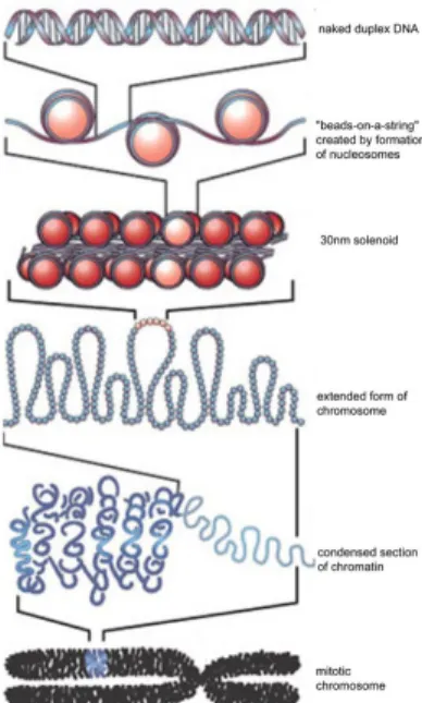
Eukaryotic genome needs to t in the small volume of the nucleus while being accessible to the DNA binding factors that control gene expression. Nucleosomes, which occupy∼75−90of the genome [9], are the basic building

blocks of the chromatin structure which is specially evolved to achieve in this goal. Nucleosomes are formed by approximately 147bps of DNA wrapping around a histone octamer, which contains two copies of each of the core histones: H2A, H2B, H3, and H4 [10]. The 10-50bp long stretches of DNA that run between nucleosomes are referred to as linker DNA. Figure 1.1 shows the hierarchical chromatin structure. The linear arrangement of the nucleosomes along the DNA constitutes the primary packing level. With addition of H1 histone proteins, multiple histones wrap into helical structures called chromatin bers which eventually form chromosomes [7].

Transcription factors (TFs) are DNA binding proteins which promote or inhibit gene expression. The net expression outcome is dependent on the concentrations and binding anities of these factors in the cell [8]. DNA binding domains of the TFs are specialized in recognizing and binding ener-getically preferable locations of the genome which are called as binding sites. The proteins which lack DNA binding domains, e.g. coactivators, chromatin remodelers, histone acetylases, deacetylases, kinases, methylases, are not la-belled as transcription factors even though they might play important roles in gene expression regulation [11].

(7)

CHAPTER 1. INTRODUCTION 7

Figure 1.1: Chromatin structure which enables eukaryotic genomic DNA to t into the nucleus of the cell while being accessible to DNA binding factors that control gene expression. DNA is wrapped around histone octamers form nucleosomes which are connected by linker DNA [35].

In general, the compactness of the chromatin is inversely proportional to DNA accessibility of the DNA binding factors. In other words, the more tightly packaged the DNA, the harder it is for the transcription factors and other DNA binding proteins to access DNA and perform their functions [7]. Even though some examples have been reported for congurations where TFs are able to bind to nucleosomal DNA [1], in most cases TFs cannot bind nu-cleosomal sequences and hence compete with nucleosomes for DNA access. Additionally, binding sites of several TFs that control the expression of the same gene may be overlapping. This again motivates a competition between dierent TFs. Consequently, in addition to the TF binding preferences, the sites to which TFs can bind also depend on the competitions between TFs and nucleosomes as well as the competitions among TFs[2]. Cellular concentra-tions and binding anities of these factors generally determine the winners of these races. Likewise, nucleosome organization is determined by multiple fac-tors, including the competition with these site specic DNA-binding proteins, DNA sequence preferences of the nucleosomes and active chromatin remod-ellers that reposition or remove nucleosomes [12, 72]. Due to the competitive binding between TFs and nucleosomes, the organization of nucleosomes play a signicant role on transcriptional gene expression regulation.

(8)

1.1 TF Binding Discovery and Prediction

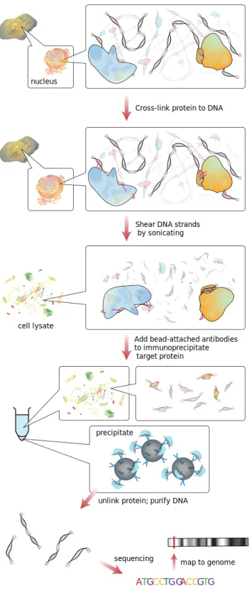
Many studies have been conducted on both transcription factor binding site (TFBS) discovery and prediction, and nucleosome positioning. Most of the computational approaches to TFBS analysis employ position weight matrices (PWMs) which quantitatively represent TF binding motifs [13](see [14] for a review). However, since TFBSs are usually short and the sequence changes at many positions of the binding sites are generally tolerated by TFs, with these methods suitable sequences are found excessively leading to low accuracy predictions. It is even claimed that, in a human cell most computationally predicted TFBS are not available for binding [13]. Many methods that point out this high false positive rate have been proposed in the literature [1519] and more exible models are suggested for the prediction of TFBSs [2025]. Other than the computational methods, high-throughput experimental methods such as chromatin immunoprecipitation with DNA microarray (ChIP-Chip) [26, 27], chromatin immunoprecipitation with massively parallel DNA sequencing (ChIP-Seq) [28] have been developed for mapping of protein bind-ing events. Since an array is restrained to a xed number of probes, ChIP-Seq has gained popularity over ChIP-Chip as the sequencing cost has decreased over time.Currently ChIP-seq is the major TF binding mapping method used in the ENCODE project. Figure 1.2 displays the ChIP-Seq workow.

In the ChIP-Seq protocol, rst the target protein is cross-linked with the DNA site it binds to. Then, the cells are lysed and the DNA is sheared by sonication or by using endonuclease enzymes. This brings about chunks of protein-DNA complexes, where the double-stranded DNA is generally 1 kb or less in length [31]. In the next step, only the complexes with the protein of interest are ltered out by using an antibody specic to the target pro-tein. The cross-linking of protein-DNA complexes is reversed and the DNA strands are puried. Oligonucleotide adaptors are then added to the small stretches of DNA that were bound to the target protein to enable massively parallel sequencing. Finally, after size selection, all the resulting ChIP-DNA fragments are sequenced simultaneously using a genome sequencer [31].

In principle, a pool of DNA fragments enriched for the target protein's binding sites should be produced at the end of the ChIP protocol. High-throughput sequencing of these fragments generates millions of short tags which are later mapped to the reference genome [33]. Due to the repetitive regions of the genome, some of these tags may be mapped to multiple loca-tions. This should be taken into account during the downstream analysis.

(9)

(10)

For single-end sequencing, the average fragment size is estimated by the distribution of distances between reads on the positive and negative strands and each read is extended to the average fragment size, while for paired-end sequencing, the distance between the paired-paired-end reads denes the actual length of each fragment. In order to identify the protein binding sites, ChIP-Sek peak nders identify genomic locations where mapped sequence tags are enriched and specify some criteria to distinguish the signicantly enriched sites. Various approaches has been proposed for this task, e.g., identifying regions where extended sequence tags overlap, sliding windows algorithm for nding xed width windows in which the number of tags are enriched, and searching bimodal pattern in the strand-specic tag densities (for a review of peak calling programs see [33]).

1.2 Nucleosome Positioning

Non overlapping positions of the nucleosomes on the DNA constitutes the nucleosome conguration of a cell[36]. Higher organisms have varying nucle-osome congurations in dierent cell types and even in a specic cell sample, the exact positions of the nucleosomes within each cell may deviate around a most preferred position. This variance of nucleosome positions within each cell in a cell population is referred to as fuzziness [37]. Nucleosome position-ing aims to assess the most preferred positions, fuzziness and the occupancy values of the individual nucleosomes. Occupancy value of a nucleosome in-dicates the frequency with which this genome position is occupied by a nu-cleosome in a cell population [37]. If a nunu-cleosome is well-positioned, this means that the nucleosome is present at the same genomic location in most of the cells in the population.

There are many factors determining the nucleosome positions. These in-clude the sequence characteristics of the local DNA and the intrinsic sequence preferences of the nucleosomes, active chromatin complexes that reposition or delete nucleosomes, competition with other DNA binding factors and the eects of neighboring nucleosomes (for a review of cis and trans determi-nants of nucleosome positioning see [38]). In a cell nucleosome positions can be altered as a response to dynamic environmental factors such as heat shock or hormonal treatment [37]. Therefore, accurate positioning of nucle-osomes and studying the nucleosome repositioning mechanisms is a key to understand how chromatin elements and transcription factors collaborate to organize the cellular responses to environmental changes [39, 40].

(11)

CHAPTER 1. INTRODUCTION 11 In order to wrap around the histone octamer the DNA helix is has to ex-perience a sharp bending. Certain sequences are argued to intrinsically favor or disfavor this curving. Nucleosomes are more likely to be formed when the bending is preferred [45, 46]. Based on this observation, numerous studies have predicted in vivo nucleosome positions directly from DNA sequence, claiming that nucleosome organizations are encoded in the genomic sequence to a certain extent [4144]. With the advance of high-throughput sequenc-ing, new experimental techniques have been designed to measure nucleosome positions on a genome-wide scale.

Micrococcal nuclease (MNase) digests chromatin at DNA sites that are not occupied by nucleosomes, because linker DNA in between nucleosomes is more exposed to the nuclease while nucleosome covered sequences are better protected from digestion [48]. Figure 1.3 illustrates the digestion process. This step introduces some biases to the experiment results, because MNase has a sequence preference to having TA/AT dinucleotide as its cleavage site [49, 50]. Fortunately, it has been demonstrated that nucleosome protection is more eective than MNase specicity in the MNase digestion [36]. After digestion, the beads are isolated and the nucleosomal DNA is extracted for high-throughput sequencing. The sequenced reads are again mapped to the reference genome, followed by some normalization steps. Nucleosomes are then positioned according to the peaks of the coverage prole, just as in the ChIP-seq peak calling process. However, the resulting coverage prole generally exhibits many blurry peaks which involves overlapping and am-biguous nucleosome positions [34]. This is due to three main reasons: rstly, MNase sequence preferences cause some DNA fragment length variation from the actual nucleosomal DNA size, which is hypothetically 147bp [54]. Sec-ondly, considering that MNase is a strong enzyme, the digestion outcome is very easily aected by the MNase concentration and incubation time [5153]. Thirdly, since it is not possible to locate the nucleosomes cell by cell with the current technologies, the deviation in the nucleosome positions between cells is directly reected in the experimental results obtained from a population of cells[54]. Several approaches and tools have been proposed to identify nu-cleosome positions from MNase-Seq data, such as peak calling [55, 56], and hidden Markov models [44] (for a recent review of nucleosome positioning methods see [60]).

(12)

Figure 1.3: MNase digests chromatin at DNA sites that are not occupied by nucleosomes [47].

1.3 Problem statement

Hypothetically any DNA sequence of a certain length is a candidate binding site for a DNA binding factor. The binding probability of a factor to a site is a time-dependent dynamic variable determined by the sequence prefer-ences of the factor, its concentration in the cell at that specic time and the stochastic competitions between dierent factors. Therefore, it would be a more realistic view of the DNA-protein interactions if the genomic positions were annotated as binding sites using a probability interval. However, cur-rent available models generally announce the positions to be either binding sites or not[2].

Secondly, most of the models of genome binding do not consider dierent types of factors together simultaneously even though considering the compe-tition between dierent factors would yield more accurate locations for both the nucleosomes and the TF binding sites [2]. In addition, methods that model the competitive and combinatorial binding pattern of transcription factors and nucleosomes at genomic regulatory regions would be benecial for revealing the complex mechanisms of gene expression regulation. The quantitative models proposed for predicting this complex combinatorial code generally use the binding anities and concentrations of the DBFs in the cell [16]. These models might work well in lower organisms under

(13)

thermody-CHAPTER 1. INTRODUCTION 13 namic equilibrium conditions but when modeling actual in vivo binding we have to consider the ATP-driven chromatin remodelers capable of actively repositioning, reconguring or ejecting nucleosomes [7], the binding cooper-ativity among transcription factors [8] and the environment of the cell with ATP-driven molecular components functioning against thermal equilibrium [57]. Moreover, the challenge of correctly determining DBF concentrations in the cell makes the application of these methods troublesome [2].

In this study we propose a probabilistic model for generating the combi-natorial occupancy prole [2] of TFs and nucleosomes in a cell sample. Our model uses Chip-Seq and MNase-Seq data sets of the TFs and nucleosomes as input which intrinsically reects the direct and indirect eects of the fac-tors related with DBF positioning. To our knowledge, ours is the rst study which explicitly models the combinatorial conguration of multiple DBFs by the use of the high-throughput sequencing data.

1.4 Structure of the Thesis

Chapter 2 represents the materials and the enrichment analysis we performed on ENCODE ChIP-Seq and MNase-Seq GM12878 cell line data which is prepared by using human lymphoblastoid cell type. Chapter 3 explains our proposed method in detail and Chapter 4 displays the experiment results. Finally Chapter 5 discusses about our ndings and concludes the study.

(14)

Chapter 2

Materials

In our experiments we used the publicly available GM12878 cell line human ChIP-Seq and MNase-Seq data sets released by the ENCODE project [58]. GM12878 is a lymphoblastoid cell line produced from the blood of a female donor with northern and western European ancestry by EBV transformation [59]. It is one of the two cell lines (other one is K562) for which MNase-Seq data is published. Currently there are 98TFs for which ChIP-Seq data

is published in this cell line. The 46 TFs that we used in our experiments

are: ATF2, ATF3, BCL3, BCL11A, BCLAF1, CEBPB, CREB1, CTCF, EBF1, EGR1, ELF1, ETS1, FOXM1, GABPA, IRF4, MEF2A, MEF2C, MTA3, NFATC1, NFE2, NFIC, NRF1, NRSF, PAX5, PBX3, PML, POL2, POL24H8, POU2F2, PU1, RAD21, RFX5, RUNX3, RXRA, SIX5, SP1, STAT1, STAT5A, TAF1, TBP, TCF3, TCF12, USF1, YY1, ZBTB33, ZEB1.

2.1 Data Preprocessing

2.1.1 ChIP-Seq Data Preprocessing

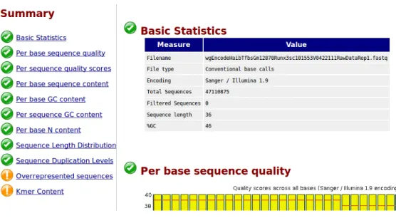
We downloaded raw ChIP-Seq data les from UCSC downloads server [61] in .fastq format and used FastQC [62] to perform quality control checks to ensure that the raw data looks good and there are no problems or biases in our data. FastQC provides a QC report which can spot problems which originate either in the sequencer or in the starting library material. Figure 2.1 displays an example FastQC report summary for the raw data le of TF RUNX3. Most of the TFs we used had high quality data according to FastQC analysis reports. For some TFs, there were overrepresented sequences which were reported to be the adapter sequences.

(15)

CHAPTER 2. MATERIALS 15

Figure 2.1: FastQC report summary example.

We removed such sequences that were ligated to the 5' or 3' ends of the library reads by the use of Cutadapt [63] software with the -q 20 -m 36 options which enabled us to trim low-quality ends from reads before adapter removal and discard trimmed reads that are shorter than 36bps.

After quality check and adapter removal, we aligned the library reads to the reference genome NCBI GRCh37 (hg19) with the Bowtie software [64]. Reads that were mapped to more than one single location were discarded. Following that, rst we converted resulting .sam format les into .bam les with Samtools view software [65] and then used Samtools rmdup to re-move the duplicate reads. Duplicate removal is important for handling the possible amplication and sequencing errors [55]. Finally, we converted the duplicate removed .bam les into .bed format which is the input le format of our tool.

In our model we use the reads in 1bp resolution. In other words, each read is represented by its 5' end coordinate. Samtools only retains the read with highest mapping quality if multiple reads have identical coordinates for their 5' and 3' ends and the reads with identical 5' end positions are kept when their 3' ends are dierent. Considering the trimming steps in our preprocessing procedure, we only keep one of the reads which have identical 5' positions and discard the others. Therefore, the occupancy value of each base pair is at most 2 (1 read mapped to the positive strand and 1 read mapped to the negative strand).

Inputs to our implementation contain the MACS summit reports for the considered TFs. In each of these reports, in addition to the peak summit locations, MACS announces the average fragment length of the ChIP-seq

(16)

CHAPTER 2. MATERIALS 16 library. We read that value and shift the reads in the 3' direction by half of the fragment length to locate the center of each fragment. As a last step, the shifted 1bp resolution reads are binned (default bin size is 5bp ) and the number of reads in each bin is used in the model.

2.1.2 MNase-Seq Data Preprocessing

During sonication or endonuclease digestion some regions of open chromatin are preferentially cut. This preference and errors during sequencing generate fragments which are mapped to non-specic background regions throughout the genome. Therefore, the reads in a ChIP sample contains some back-ground noise reads as well as the enrichment signal reads. In order to reduce the eect of the noise in the data, the experiment signal should be analyzed considering a reference sample. There are two basic methods to generate the control data for the ChIP-seq experiments. Both of these methods use the cells from the same sample as used in the ChIP sample. In the rst method, the input DNA is produced by cross linking and fragmenting the cell DNA without immunoprecipitation. The second method includes immunoprecipi-tation step but uses an antibody that has no specicity to any protein. The control data obtained by following the second technique is called IgG con-trol. Input control ChIP-seq data is published for the ChIP-seq that we used in our experiments. We preprocess the control data with the same steps used in preprocessing the sample data. In order to normalize the control data, we calculate the ratio between the total control tag count and total sample tag count, and multiply the binned control signal with this ratio before subtracting it from the binned sample signal.

-For the preprocessing of ENCODE GM12878 cell line MNase-Seq data, we followed the same steps explained in Section 2.1.1, except that for this data set reads and index were in colorspace and necessary arguments (-c for cutadapt and -C for bowtie) were specied to align the reads to the reference genome hg19.

2.2 Data Enrichment Analysis

2.2.1 ChIP-Seq Data Enrichment Analysis

We performed ChIP-Seq read enrichment analysis around the peak summits detected by MACS [66] for all of the TFs we considered throughout our exper-iments. When we inspected the read distributions in 800bp regions centered at 400 most signicant peak summits of MACS, we observed that the number

(17)

CHAPTER 2. MATERIALS 17 of reads mapped to the + strand are enriched in a [−w,0] window and the

number of reads mapped to the - strand are enriched in a[0, w]window where

w was a number close to the average fragment length reported by MACS.

Therefore, when we shifted the 5' end positions of the reads by w/2, the

cu-mulative signal in a w bp window centered at the summits was signicantly

enriched compared to the background. This observation is compatible with the assumptions of most of the peak calling algorithms [33]. As an example of these analyses, Figure 2.2 displays the heat maps for the 1bp resolution read distribution in 800bp regions centered at 400 most signicant EBF1 peak summits on chromosome one that were reported by MACS and Figure 2.3 shows the average density proles of these 400 regions. MACS reports the average fragment length of this TF ChIP-Seq library to be 103bp, and accordingly we see that there is a signicant enrichment in a ∼ ±100 region

centered at the summits.

2.2.2 MNase-Seq Data Enrichment Analysis

We also performed a similar analysis on the MNase-Seq data. For that purpose, we ran DANPOS [37] software on MNase-Seq data for ENCODE GM12878 cell line, chromosome one and after ordering the nucleosome sum-mits according to their p-values, we analyzed the 1bp resolution read dis-tribution at the regions which are centered at 500 most signicant summit positions.

Although nucleosome size is 147bp in higher eukaryotes, due to the noisy nature of existing nucleosome positioning data, the real size of DNA frag-ments after MNase digestion vary from∼120bp to210bp [12, 37]. Moreover,

MNase-Seq data is more scattered compared with Chip-Seq data because of the mobility of the nucleosomes in a cell population. Since we had single-end sequenced MNase-Seq data, in order to nd the average fragment length, we measured the phase shift between the + strand read density and - strand read density by calculating the cross correlation between + and - density signals.

Figure 2.4 displays the heat maps for 1bp resolution read distribution in 600bp regions centered at 500 signicant nucleosome summit positions

detected by DANPOS and Figure 2.5 shows average 1bp read density proles of these regions. In Figure 2.5a, we observe the phase-shift value between + and - strand density signals to be ∼200bp. When the reads were shifted

by 100bp, the enriched regions of the two signals overlap as shown in Figure 2.5b. In this gure, we see that the number of fragment centers of MNAse-Seq reads are enriched in a ∼ 75bp window. These MNase-Seq enrichment

(18)

(a) Reads mapped to + strand.

(b) Reads mapped to - strand.

(c) Reads mapped to both strands.

Figure 2.2: Heat maps displaying the 1bp resolution read distribution in 800bp regions centered at peak summits (most signicant 400) for EBF1 protein detected by MACS.

(19)

(a) Fragments are unshifted.

(b) Fragments are shifted by d₂, which is 51bp for EBF1.

Figure 2.3: Average 1bp resolution read density proles in 800bp regions centered at MACS reported peaks summits for EBF1.

(20)

(a) Reads mapped to + strand.

(b) Reads mapped to - strand.

(c) Reads mapped to both strands.

Figure 2.4: Heat maps displaying the 1bp resolution read distribution in 600bp regions centered at nucleosome summit positions (most signicant 500) detected by DANPOS.

(21)

(a) Fragments are unshifted.

(b) Fragments are shifted by half of the phase shift value between + strand signal and - strand signal.

Figure 2.5: Average 1bp read density proles in 600bp regions centered at DANPOS reported nucleosome summits.

(22)

Chapter 3

Model Description

3.1 Model Description

LetΘ = {θ1_{, θ}2_{, ..., θ}M_}be the set of _M DBFs consisting of nucleosomes and

M −1 dierent TFs where θi denotes the DBF i. S = (s1, ..., sL) is the

genome sequence of the nucleotides in the inspected region which is L bp

long. For notational simplicity, Lis expected to be a multiple of the bin size n which is 5bp by default.

Q, which stands for the number of binding sites in S, is unknown. All

binding sites of any DBF θi are assumed to be _dδi

ne ×n bp long where δ i

is the average motif length of DBF θi. Q = c denotes that there are c

non-overlapping binding sites which can belong to any of the M DBFs. K =

{k1, ..., kc} ⊂S is the set of start positions of thesecnon-overlapping binding

sites. Finally, π ⊂ {θ1, ..., θM}c _{stands for a conguration indicating which}

DBFs hold which binding sites. A tuple consisting of congurationπwith the

corresponding setK, can be referred to as a state. For instance, whenc= 3,

M = 7 and S = (4567, ...,4700) on chromosome one, one such conguration

might be π = (θ3_{, θ}7_{, θ}3₎ _{with the corresponding start positions} _K ₌_{_k 1 = 4569, k2 = 4615, k3 = 4690} assuming dδ 3 ne ×n≤15 and d δ7 ne ×n≤75.

Read density proles of Chip-seq and MNase-seq data, for which the analysis results were presented in Chapter 2, can be used for assessing the probability of a conguration π with a specied set K. We can denote the

set of binned read density proles of DBFs' high throughput data mapped to S as D = {d1, ..., dM} where di stands for the binned read distribution

prole of high throughput data for θi along the inspected region _S. That is,

when xi,j represents the number of 1bp resolution reads mapped to binj for

θi_:

(23)

CHAPTER 3. MODEL DESCRIPTION 23

di = (xi,1, xi,2, ..., xi,L

n). (3.1)

Using Bayes' rule, the probability of the binding site positions K and

conguration π, given D is:

P(K, π|D) = P(D|K, π)P(K, π)

P(D) (3.2)

Since D = {d1, ..., dM}, when we assume conditional independence

be-tween read distribution proles given a particular conguration and start positions Equation 3.2 can be rewritten as:

P(K, π|D) = P(K, π|d1, ..., d) = P(d1, ..., dM|K, π)P(K, π) P(d1, ..., dM) = P(d1|K, π)...P(dM|K, π)P(K, π) P(d1, ..., dM) (3.3) The peak summits reported by MACS provide us empirical prior infor-mation about the number of possible binding sites of each TF. The prior probability of TF θi havingbi number of binding sites in state(K, π)is

mod-eled by a Poisson distribution with λi being equal to the number of peak

summits reported by MACS for the inspected region. For the nucleosomes, we lack such information and we model the prior probability distribution of the number of nucleosomes in the Lbp long region as Unif[0,₁₅₀L ]. Therefore,

the prior P(K, π)is:

P(K, π) = Poi(b1|λ1)...Poi(bm−1|λM−1)Unif[bm|0,

L

150] (3.4)

P(di|K, π) denotes the marginal likelihood of the binned read density

prole of DBF θi _along _S_{, given conguration} _π _{and the set of binding site}

start positions K.

Based on our observations explained in Chapter 2, we can conclude that

di is composed of bins belonging to enriched and background regions. For

TFs, the enriched regions are assumed to be fragment length long windows centered (referred to as enriched windows hereinafter) at the binding sites and are of equal length for all of the binding sites of a specic TF. Whereas, for nucleosomes, the middle 75bp window is considered to be the enriched region of a nucleosome site of 150bp long. When two or more binding sites of a TF are close to each other, the enriched regions around these binding sites

(24)

CHAPTER 3. MODEL DESCRIPTION 24 overlap forming combined enriched regions (dened later). The likelihood

P(di|K, π)is the product of the likelihood of the enriched binsP(di−en|K, π)

and the likelihood of the background bins P(di−bg|K, π)

P(di|K, π) =P(di−en|K, π)P(di−bg|K, π). (3.5)

Note that, for each di, (K, π) denes the enriched and background bins.

Instead of P(di−en(K,π)|K, π) and P(di−bg(K,π)|K, π) we write P(di−en|K, π)

and P(di−bg|K, π)for notational brevity.

Negative binomial distribution is a popular choice for modelling back-ground read counts [67]. We model the distribution of the backback-ground bin read counts with poisson distribution with gamma prior. The poisson and gamma distributions being conjugate, the marginal likelihood can be calcu-lated in closed form using the negative-binomial distribution [68]. For θi, if

we denote the set of indices corresponding to background regions at state

(K, π) asIi−bg(K, π)and assume an independent gamma prior for each bin,

then the the background likelihood P(di−bg|K, π) can be calculated as the

product of the likelihood of the read counts in each background bin:

We have used the empirical Bayes approach and estimated the background

N B parameters by using the bin read counts in a [-2500, + 2500] interval

around the inspected region. For TFs, the bin count values of all bins in this interval are used for background parameter estimation. However, considering that 75 to 90 percent of eukaryotic genomic DNA is packaged into nucleo-somes and each ∼210bp (147 for the particle plus ∼60bp for the one linker

region ) nucleosomal region has a corresponding 75bp enriched window in our model, we have used the 85% lowest bin read counts to infer the parameters

(25)

CHAPTER 3. MODEL DESCRIPTION 25 Let Ti,j denote the total read count in enriched window j centered at a

binding site of DBF θi _{. Based on our observations for distribution of the}

total number of reads in enriched windows centered at peak summits reported by MACS, we model the distribution of Ti,j with poisson distribution with

gamma prior. GivenTi,j, the read counts of the individual bins in the enriched

window, Yi,j, are assumed to follow the multinomial distribution with bin

level probabilities Φwhich describes the peak shape around a single binding

site1_{. Peaks in real data vary in widths, heights, and shapes, possibly due to}

various biological and technical factors. Therefore, we use a dirichlet prior forΦwhich provides a exible model to allow the heterogeneity and variation

in the peak shapes.

When there arebi non-overlapping enriched windows ofθiin state(K, π),

the likelihood of the combination of the enriched regions P(di−en|K, π) is:

MN(Yi,j|Φ, Ti,j)Dir(Φ|α∗)dΦ

(3.9) = bi Y j=1 NB(Ti,j|α 0

, β0)·Polya(Yi,j|Ti,j, α∗

(3.10) In equation 3.10,(α0, β0)are parameters of the gamma distribution which

is the prior for λen. α∗ stands for the prior dirichlet parameters which

speci-es the template unimodal peak prole. Since each bin has its own specied multinomial probability value, number of the parameters in α∗ is equal to

the number of bins in an enriched window. (This bin count is equal to

dfragment length_{bin size} e for TFs andd_{bin size}75 efor nucleosomes.) For enriched windows

containing only one binding site, to set α∗, we calculate the binned read

distribution signals in windows centered at the 4000 most signicant peak summits detected by MACS ( for TFs) or 8000 DANPOS nucleosome peak summits. Then, we estimate α∗ by nding the values which maximizes the

likelihood of this array of signals. Since there is no closed-form solution for

1_{Note that} _Y_i,j _{is a set of consecutive read counts from} _d_i_,i.e., _Y_i,j ₌

(26)

CHAPTER 3. MODEL DESCRIPTION 26 the maximum-likelihood estimate of Dirichlet-multinomial compound distri-bution (also known as multivatiate Polya distridistri-bution) parameters, we nd the maximum-likelihood estimate of α∗by using the L-BFGS-B optimization

algorithm [74] implemented in Python scipy.optimize module. However, for some DBFs we have observed that the average of this signal array does not project the read distribution around individual peak summits, which is in general a unimodal peak centered at the peak summit. Therefore, we de-cided to use a Gaussian shaped function exp(−(x_2(2z)−z)22) for regularizing α

∗ while making sure that sum of the parameters in resulting α∗ is equal to the

sum of the parameters in maximum likelihood estimate, i.e., if the number of bins in the enriched window centered at a single binding site is 2z then:

α∗ = (α∗₁, α∗₂, ..., α∗_2z) (3.11)

α∗_j = exp(−(j−z)

2

8z2 ) (3.12)

In some states where two or more binding sites of the same TF are closely located, the enriched windows, each of which is centering at a dierent bind-ing site, may overlap. In these cases, the prior Dirichlet parameters for the combined enriched window are calculated as a combination of the dirichlet parameters of the individual enriched windows such that the corresponding parameters of the overlapped bins are summed up.

Integrating out the enriched window specic multinomial probabilitiesΦ,

we can obtain the marginal bin counts distribution conditional on total count of the enriched windowTi,j. This marginalization is computed in closed form

by Polya distribution.

3.2 Monte Carlo Markov Chain Estimation

In addition to the fact that calculating the necessary normalization factor

P(D)is extremely dicult, computing the posteriorP(K, π|D)for allK and π is impossible. However, we can draw samples from the target distribution

by using Markov Chain Monte Carlo (MCMC) [69] framework which is scaled well with the dimensionality of the sample space. For this purpose we use a Metropolis-Hasting algorithm by which we construct a Markov chain such that its unique stationary probability distribution P((K, π)) converges to

our target distribution P(K, π|D) irrespective of the choice of the initial

distribution.

A distribution is said to be stationary, with respect to Markov chain if each step in the chain leaves the distribution stationary [69]. That is,

(27)

CHAPTER 3. MODEL DESCRIPTION 27 with transition probabilities T((K0, π0),(K, π)), the distributionP((K, π))is

stationary if :

P((K0, π0)) = X ((K,π))

T((K0, π0),(K, π))P((K, π))

In order to guarantee an acceptable approximation of the simulated model, the Markov chain should have a unique stationary distribution. It is guar-anteed thatP((K, π))is a unique stationary distribution when the following

two conditions are met:

• existence of stationary distribution: Detailed balance condition

is a sucient but not necessary way for ensuring that there exists a stationary distribution P((K, π)). A stationary distribution requires

that each transition T((K0, π0),(K, π)) is reversible. In other words,

for every pair of states(K, π),(K0, π0), the probability of being in state (K, π)and transit to the state(K0, π0)must be equal to the probability

of being in state (K0, π0) and transit to the state(K, π):

P((K, π))T((K0, π0),(K, π)) =P((K0, π0))T((K, π),(K0, π0))

This preliminary constraint on T((K0, π0),(K, π))is called irreducibility.

Irreducibility property ensures that for any state of the Markov chain, there is a positive probability of visiting all other states. That brings transition kernel T in allowing for moves all over the state-space. In the discrete case

that means no matter what the starting state is, the Markov chain has a positive probability of eventually reaching any region of the state space.

• uniqueness of stationary distribution: This is guaranteed by

er-godicity property, which requires that every state must be:

aperiodic: This property ensures that the system does not return to the same state at xed intervals.

positive recurrent: This property ensures that the system will return to the same state with nonzero probability and expected recurrence time is nite.

The notion of positive recurrency is necessarily satised for irreducible chains on a nite space [69]. Therefore, it can be shown that a nite state irreducible Markov chain is ergodic if it has an aperiodic state. In other words, a model is said to hold the ergodic property if there is a nite number N such that any state can be reached from any other

(28)

CHAPTER 3. MODEL DESCRIPTION 28 will converge to the same stationary distribution P((K, π)) no matter

what the initial state is.

Based on these requirements, we dene the proposal distributionG((K0, π0)|(K, π)),

which proposes new state (K0, π0) based on the current state (K, π), as

fol-lows:

• Move 1: with probability p1, propose a new occupied and

non-overlapping binding site to a DBF which is randomly chosen among DBFs that are eligible for having an additional non-overlapping bind-ing site in the current state. To increase acceptance rate, proposed binding site is selected by the use of a multinomial probability distri-bution which always has non-zero set of parameters that are directly proportional to the chosen DBF's binned read density prole at the available non-occupied, non-overlapping binding sites.

• Move 2: with probabilityp2, delete a randomly chosen binding site of

a randomly chosen DBF which has a binding site in the current con-guration. Chosen binding site is selected by the use of a multinomial probability distribution which always has non-zero set of parameters that are directly proportional to the binned read density prole of the DBF at its current binding sites.

• Move 3: with probability p3, shift a randomly chosen binding site of

a DBF by 1 bin to the left provided that a binding site of this DBF exists and the shifted position does not overlap with any other binding sites

• Move 4: with probability p4, shift a randomly chosen binding site of

a DBF by 1 bin to the right provided that a binding site of this DBF exists and the shifted position does not overlap with any other binding sites

• Move 5: with probability p5, swap randomly chosen binding sites of

two TFs with equal motif lengths which have at least one binding site in the current conguration

where

p1 >0, p2 >0, p3 >0, p4 >0, p5 >0

(29)

CHAPTER 3. MODEL DESCRIPTION 29 The candidate sample is accepted with probability:

A((K0, π0),(K, π)) = min 1,P(K 0_{, π}0_|_D₎ P(K, π|D) × G((K, π)|(K0, π0)) G((K0_{, π}0₎_|₍_{K, π}₎₎ = min 1,P(d1|K 0_{, π}0₎_...P₍_d M|K0, π0)P(K0, π0) P(d1|K, π)...P(dM|K, π)P(K, π) × (3.13) G((K, π)|(K0, π0)) G((K0_{, π}0₎_|₍_{K, π}₎₎ (3.14) If the candidate sample is accepted at time t, then the next state is

(K0, π0) at time t+ 1, otherwise the candidate sample (K0, π0) is discarded

and the state at t+ 1 is set to (K, π) and another sample is drawn from the

distributionG((K0, π0)|(K, π)). That is, when a candidate sample is rejected,

the previous sample is included instead in the nal list of samples, leading to multiple copies of the samples.

The resulting chain satises the irreducibility and aperiodicity constraints which are required for a unique stationary distribution. Since the inspected region is nite, the number of all possible DBF binding congurations is nite. We assume that each one step move has a non-zero probability which makes any state(K, π)be reached from any other state(K0, π0)by following a

nite number of moves proposed by G. Therefore, irreducibility of the chain

holds. Aperiodicity of our chain is also assured because in each step, there is a positive probability of choosing the reverse moves of the moves that have been made so far which makes the probability of moving from (K, π)back to (K, π)in two or more number of steps non-zero. For instance at state(K, π)

the chain has a non-zero probability of moving to state (K0, π0) and stay at

this state for one or more steps and return back to state (K, π).

3.3 Probabilities of Forward and Reverse moves

In a region consisting of r = L_n number of bins, B = (b1, ..., bM) vector

contains the number of non-overlapping binding sites for each of theM DBFs

in this region in the current state. For simplicity, lets suppose each DBF has a motif length equal to the bin size, and thusbiis equal to the number of bins

occupied by the binding sites of DBF θi. When computing the probability

in Equation 3.13, G((K0, π0)|(K, π))andG((K, π)|(K0, π0))can be calculated

for 5 possible moves of the proposal distribution as follows:

Forward and Reverse Move Probabilities of Move 1:

In this simplied case where each DBF has a motif length equal to the bin size, the expression r − PM

(30)

CHAPTER 3. MODEL DESCRIPTION 30 binding sites in the current state. The probability of a candidate binding site to be selected is directly proportional to the binned read count of the selected DBF at this location. By the use of the multinomial distribution, candidate non-occupied, non-overlapping binding site at kth bin is selected

with non-zero probability xik+2 P

s(xis+2) where xi,s represents the number of 1bp

resolution reads mapped to bin s for θi_{. Therefore, the forward and reverse}

move probabilities of addition move are:

G((K0, π0)|(K, π)) = p1 m1 xik+ 2 P s(xis+ 2) (3.15) G((K, π)|(K0, π0)) = p2 m0₂ xik+ 2 Pb0z s (xis+ 2) ! (3.16) Here m1 represents the number of DBFs which are eligible for having

an additional binding site in the current state. Therefore, it is equal to the number of DBFs whose motif length is smaller or equal to any of the available free spaces in the current binding conguration. When motif lengths of DBFs are some multiples of the bin size, the number of candidate sites should be calculated accordingly. m0₂ is the number of DBFs which has at least one

binding site in the proposed state and b0_z is the number of binding sites of

the selected DBF in the proposed state.

Forward and Reverse Move Probabilities for Move 2:

G((K0, π0)|(K, π)) = p2 m2 xik+ 2 Pbz s (xis+ 2) ! (3.17) G((K, π)|(K0, π0)) = p1 m0₁ xik+ 2 Pr−Pm_j₌₁b0_j s (xis+ 2) ! (3.18) Forward and Reverse Move Probabilities for Move 3:

G((K0, π0)|(K, π)) = p3 m3 1 b∗ z (3.19) G((K, π)|(K0, π0)) = p4 m0₄ 1 b∼0 z (3.20) Forward and Reverse Move Probabilities for Move 4:

G((K0, π0)|(K, π)) = p4 m4 1 b∼ z (3.21)

(31)

CHAPTER 3. MODEL DESCRIPTION 31 G((K, π)|(K0, π0)) = p3 m0₃ 1 b∗0 z (3.22) In equations 3.19-3.22, m3 and m 0

3 are the number of DBFs which have

at least one binding site eligible for a left shift in current and next state respectively. Similarly, m4 and m

0

4 are the number of DBFs which have at

least one binding site eligible for a right shift in current and next state. In these equations, b∗_z andb∗_z0 denote the number of binding sites of the selected

DBF which can be shifted to left in current and proposed states respectively. Likewise,b∼_z and b∼_z0 denote the number of binding sites of the selected DBF

which can be shifted to right in current and proposed states. Forward and Reverse Move Probabilities for Move 5:

Forward and reverse move probabilities of move 5 are always equal to each other, which can be computed by the following function:

G((K0, π0)|(K, π)) = G((K, π)|(K0, π0)) = p5 m2(m2−1) 1 bx 1 by = p5 m0₂(m0₂−1) 1 b0_x 1 b0_y (3.23) Againm2 andm 0

2 are the number of DBFs which has at least one binding

site in the current and proposed state respectively. Since the total number of occupied binding sites do not change with this move, m2 is always equal

to m0₂. Likewise, bxand by are the number of non-overlapping binding sites

of θx _and _θy _{which do not change in the proposed state.}

The sequence of samples obtained by the employment of our proposal distribution is used to approximate the posterior distribution P(K, π|D).

Each sample denes a congurationπ with the corresponding start positions K which together specify the binding sites of the M dierent DBFs and the

sites which are not bound by any of the DBFs. When all of the collected samples are taken into account, anM×L

n probability matrix Ais calculated

where each element aij indicates the binding probability of θi to the sites

in the jth bin of the considered region. Since these probability values are

computed by the use if the MNase-seq and ChIP-seq data, they automatically reect the sequence preferences and cell concentrations of the DBFs as well as the eects of the competitive binding and other factors aecting DBFs' binding locations and binding frequencies.

3.4 Convergence Monitoring

Even though the chain is ergodic as shown above, it is important to monitor the convergence of the algorithm and make sure that the distribution of the

(32)

CHAPTER 3. MODEL DESCRIPTION 32 chain does not change over time. For this purpose, we periodically nd the maximum of the absolute dierence between the posterior distributions of the samples obtained by two separate chains which are run simultaneously and stop the chains when this distance is below a user dened maximum threshold.

(33)

Chapter 4

Experiment Results

We applied our model to 46 ChIP-seq data and MNase-seq data at 300 [-1000, +1000] regions around transcription start sites (TSSs) on chromosome one. Names of the TFs are listed in the Materials section. These regions are selected according to their MACS reported peaks abundance.

During our simulations, the convergence threshold for the maximum of the absolute dierence between the posterior distributions of the two separate chains is set to be between0.08−0.1. In the burn-in period, the rst200,000

samples are thrown away. The maximum number of acquired samples is set to be 26,000,000, therefore if the threshold is not reached in the specied

running time, the posteriors of the chains are calculated based on this number of accepted samples.

To illustrate a possible outcome of our proposed method, Figure 4.1 dis-plays chain one and chain two posterior binding probabilities of 45 TFs and nucleosomes in a [-1000, +1000] interval around a TSS. In each of the sub-plots, the rst nine tracks show the probability values for the TFs, track ten is for the nucleosomes and track eleven stands for the probability values of each 5bp bin being not occupied by any of the considered DBFs.

The two chains are run as independent processes and the maximum of the absolute dierence between the chains is checked every 500 seconds by the main process. At each of these controls, if the threshold value is reached, the chains are stopped and the output posterior probability distribution is calculated by taking the mean of the two chains' posteriors. Otherwise, the algorithm runs until both of the chains accumulate at least 26,000,000

accepted samples.

(34)

CHAPTER 4. EXPERIMENT RESULTS 34

(a) Posterior probabilities of chain one.

(b) Posterior probabilities of chain two.

(35)

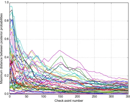
Figure 4.2: Time course maximum chain posterior dierence values of 46 DBFs.

The probability values shown in Figure 4.1 are obtained in a simulation where the convergence threshold was not reached at the end of349checks and

the acquired26,000,000samples were used to estimate the posteriors. Figure

4.2 displays the evolution of the maximum posterior dierence values of 46

DBFs through these 349 time course check points. During our simulations,

we generally observed this kind of exponential decrease in the distance values between the chains.

As another example, Figure 4.3 displays the posterior probability values of the two chains in an experiment where the convergence was reached with a threshold of 0.1. Figure 4.4 shows the convergence monitoring of this

(36)

(a) Posterior probabilities of chain one.

(b) Posterior probabilities of chain two.

(37)

Figure 4.4: Time course maximum chain posterior dierence values of 47 DBFs.

4.1 Performance Evaluation for Accurate

Bind-ing Site Detection

In order to determine the accuracy of our proposed model in detecting the binding sites of the TFs, we compared the peaks of our posterior values with MACS reported results based on the annotated TF motif sites. During these comparisons, for each TF we identied as many highest values out of the posterior probabilities as the number of peaks reported by MACS and referred the bin locations of these maximum posterior values as our predicted TF binding sites.

We used the 'factorbookMotifPos' and 'factorbookMotifCanonical' tables of the hg19 database of the UCSC bioinformatics site to obtain the positions of the annotated TF motif sites. Then, we measured the distance between the motif sites and the midpoints of our predicted binding sites, and the distance between the MACS peak summits and the motif sites. Since, some of the peaks might have been due to indirect binding to the DNA, we only considered the distance values which were below 200bp. We calculated all such distance values for 46 TFs in 300 [-1000, +1000] regions around TSSs. As

(38)

CHAPTER 4. EXPERIMENT RESULTS 38 an example, Figures 4.6 and 4.7 display the histograms of the distance values between the predicted binding locations and ELF1, YY1 motif sites in the inspected 300 regions respectively. For these TFs, we see that in general our maximum posterior values are closer to the motif sites than MACS reported binding sites. Figure 4.5 displays the comparison of the means of these distance values for all of the considered TFs which has at least two distance measurements (smaller than 200bp) in total. With these comparisons we again observe that, our predictions are usually closer to the motif sites than the MACS reported peak summits.

Figure 4.5: Mean distance values for each TF between MACS reported bind-ing sites-motif sites versus our predicted bindbind-ing sites-motif sites.

(39)

(a) Histogram for the distance values between the MACS ELF1 peak summits and anno-tated ELF1 motif sites.

(b) Histogram for the distance values between our method’s predicted binding sites and annotated ELF1 motif sites.

Figure 4.6: Histograms for the distance values, which are smaller than 200bp, between ELF1 motif sites and the binding site predictions.

(40)

(a) Histogram for the distance values between the MACS YY1 peak summits and anno-tated YY1 motif sites.

(b) Histogram for the distance values between our method’s predicted binding sites and annotated YY1 motif sites.

Figure 4.7: Histograms for the distance values, which are smaller than 200bp, between YY1 motif sites and the binding site predictions.

(41)

Chapter 5

Discussion

In this study, we proposed a probabilistic model for the organization of DBFs on DNA using ChIP-seq and MNase-seq data. Our model takes into account the combinatorial nature of binding probabilities of DBFs to DNA sites, and annotates the binding sites using a probability interval. Moreover, it includes the competition between dierent factors, which, according to our results, increase the precision of binding site estimates. Unlike thermodynamic mod-els, which also aim to model the combinatorial binding pattern of the DBFs, our model does not assume thermodynamic equilibrium conditions and in-trinsically considers in vivo conditions by the use of the high-throughput ChIP-seq and MNase-seq data. Finally, our proposed method is applicable on high number of DBFs which is an important advantage for studies that target integrated analysis of DBFs.

In our experiments, we have used high-throughput ChIP-seq data for 46 TFs and MNase-seq data for nucleosomes and analyzed 300 [−1000,+1000]

regions centered at TSSs. Throughout the experiments, we have observed ecient convergence statistics of the MCMC chains. In order to evaluate our binding site predictions, we have compared the distances between the maximums of the posterior probability distributions and MACS reported peaks with respect to the annotated motif sites. We have seen that for most of the TFs, our predictions have smaller mean distance values to the motif sites.

Our method's bottleneck is the slower mixing time to reach stationary distribution, which specically shows up during integration of high number of DBFs. Therefore, it is dicult to apply it to large genomic regions. That being said, we claim that it can be especially useful for the analysis of cis-regulatory regions like promoters and enhancers.

(42)

Bibliography

[1] V.B. Teif and K. Rippe, Calculating transcription factor binding maps for chromatin. In Proceedings of Briengs in Bioinformatics. 2012, 187-201.

[2] T. Wasson and A. Hartemink, An ensemble model of competitive multi-factor binding of the genome. Genome Res. 2009 19 (11): 2101-2112 [3] J. Gertz, ED Siggia, BA Cohen, Analysis of combinatorial cis-regulation

in synthetic and genomic promoters. Nature 2009;457:215-8

[4] X. He, MA. Samee, C. Blatti, S. Sinha, Thermodynamics-based models of transcriptional regulation by enhancers: the roles of synergistic acti-vation, cooperative binding and short-range repression. PLoS Comput Biol 6: e1000935. 2010, doi:10.1371/journal.pcbi.1000935.

[5] Tali Raveh-Sadka, Michal Levo, Eran Segal, Incorporating nucleosomes into thermodynamic models of transcription regulation. Genome Res. 2009 August; 19(8): 14801496. doi: 10.1101/gr.088260.108

[6] T. Kaplan, X.Y. Li, P.J. Sabo, S. Thomas, J.A. Stamatoyannopou-los, M.D. Biggin, M.B. Eisen, Quantitative models of the mechanisms that control genome-wide patterns of transcription factor binding during early Drosophila development. PLoS Genet. 2011 Feb 3;7(2):e1001290. doi: 10.1371/journal.pgen.1001290.

[7] B.R. Cairns, The logic of chromatin architecture and remodelling at promoters. Nature 461, 2009, 193-198 | doi:10.1038/nature08450

[8] E. Segal, T. Raveh-Sadka, M. Schroeder, U. Unnerstall, U. Gaul, Pre-dicting expression patterns from regulatory sequence in Drosophila seg-mentation. Nature. 2008;451(7178):535-40. doi: 10.1038/nature06496 [9] K.E. Van Holde, Chromatin. 1989, New York,Springer.

(43)

BIBLIOGRAPHY 43 [10] Karolin Luger, et al. Crystal structure of the nucleosome core particle

at 2.8 Å resolution, Nature 389.6648, 1997, 251-260.

[11] A.H. Brivanlou, J.E. Darnell, Signal transduction and the con-trol of gene expression. 2002 Science 295 (5556): 8138. Bib-code:2002Sci...295..813B. doi:10.1126/science.1066355

[12] N. Kaplan, I.K. Moore, Y. Fondufe-Mittendorf, A.J. Gossett, D. Tillo, et al., The DNA-encoded nucleosome organization of a eukaryotic genome. Nature 458: 362366, 2009

[13] A. Mathelier, W.W. Wasserman, The Next Generation of Transcription Factor Binding Site Prediction, PLoS Computational Biology;2013, Vol. 9 Issue 9, p1

[14] G.D. Stormo, Modeling the specicity of protein-dna interactions. Quan-titative Biology 2013, Vol:1: 115130. doi: 10.1007/s40484-013-0012-4 [15] A. Stark, M.F. Lin, P. Kheradpour, J.S. Pedersen , L. Parts, et al.,

Discovery of functional elements in 12 Drosophila genomes using evolu-tionary signatures. Nature 450, 2007, 21932. doi: 10.1038/nature06340 [16] V. Bernard, A. Lecharny, V. Brunaud, Improved detection of motifs with preferential location in promoters. Genome 53, 2010, 73952. doi: 10.1139/g10-042

[17] A. Arvey, P. Agius, W.S. Noble, C. Leslie, Sequence and chromatin determinants of cell-type-specic transcription factor binding. Genome research 22, 2012, 172334. doi: 10.1101/gr.127712.111

[18] S.J. Ho Sui, J.R. Mortimer, D.J. Arenillas, J. Brumm, C.J. Walsh, et al., oPOSSUM: identication of over-represented transcription factor bind-ing sites in co-expressed genes. Nucleic acids research 33, 2005, 315464. doi: 10.1093/nar/gki624

[19] S.J. Ho Sui, D.L. Fulton, D.J. Arenillas, A.T. Kwon, W.W. Wasser-man oPOSSUM: integrated tools for analysis of regulatory mo-tif over-representation. Nucleic acids research 35: W24552. doi: 10.1093/nar/gkm427

[20] Th. Lin, P. Ray, G.K. Sandve, S. Uguroglu, E.P.Xing, BayCis : A Bayesian Hierarchical HMM for Cis-Regulatory Module Decoding in Metazoan Genomes. In: Vingron M, Wong L, editors, RECOMB'08 Proceedings of the 12th annual international conference on Research in

(44)

BIBLIOGRAPHY 44 computational molecular biology. 2008, Springer Berlin Heidelberg, pp. 6681.

[21] L. Levkovitz, N. Yosef, M.C. Gershengorn, E. Ruppin, R. Sharan, et al., A Novel HMM-Based Method for Detecting Enriched Transcrip-tion Factor Binding Sites Reveals RUNX3 as a Potential Target in Pan-creatic Cancer Biology. PloS one 5, 2010, e14423. doi: 10.1371/jour-nal.pone.0014423

[22] R.A. Salama, D.J. Stekel, Inclusion of neighboring base interdependen-cies substantially improves genome-wide prokaryotic transcription fac-tor binding site prediction. Nucleic acids research 38, 2010, e135. doi: 10.1093/nar/gkq274

[23] P. Mehta, D.J. Schwab, A.M. Sengupta, Statistical Mechanics of Transcription-Factor Binding Site Discovery Using Hidden Markov Models. Journal of statistical physics 142, 2011, 11871205. doi: 10.1007/s10955-010-0102-x

[24] V.D. Marinescu, I.S. Kohane, A. Riva, MAPPER: a search engine for the computational identication of putative transcription factor binding sites in multiple genomes. BMC bioinformatics 6, 2005, 79.

[25] R. Durbin, S. Edddy, A. Krogh, G. Mitchison, Biological sequence analy-sis Probabilistic models of proteins and nucleic acids. Cambridge: Cam-bridge University Press, 1998

[26] B. Ren, F. Robert, J.J. Wyrick, O. Aparicio, E.G. Jennings, I. Si-mon, J. Zeitlinger, J. Schreiber, N. Hannett, E. Kanin, et al., Genome-wide location and function of DNA binding proteins. Science 290, 2000, 23062309.

[27] K.D. MacIsaac, T. Wang, D.B. Gordon, D.K. Giord, G.D. Stormo, E. Fraenkel., An improved map of conserved regulatory sites for Saccharomyces cerevisiae. BMC Bioinformatics 7, 2006, 113. doi: 10.1186/1471-2105-7-113.

[28] D.S. Johnson, A. Mortazavi, R.M. Myers, B. Wold, Genome-wide map-ping of in vivo proteinDNA interactions. Science 316, 2007, 14971502. [29] M.L. Bulyk, X. Huang, Y. Choo, G.M. Church, Exploring the DNA-binding specicities of zinc ngers with DNA microarrays. Proc Natl Acad Sci 98, 2001, 71587163.

(45)

BIBLIOGRAPHY 45 [30] By Jkwchui [CC-BY-SA-3.0 (http://creativecommons.org/licenses/by-sa/3.0) or GFDL (http://www.gnu.org/copyleft/fdl.html)], via Wikime-dia Commons

[31] O. Aparicio, J.V. Geisberg, K. Struhl, Chromatin immunoprecipitation for determining the association of proteins with specic genomic se-quences in vivo. Current Protocols in Cell Biology (University of South-ern California, Los Angeles, California, USA.: John Wiley & Sons, Inc.), 2004, Chapter 17 (2004): Unit 17.7. doi:10.1002/0471143030.cb1707s23. ISBN 0-471-14303-0. ISSN 1934-2616. PMID 18228445

[32] The ENCODE Project Consortium. An integrated encyclopedia of dna elements in the human genome. Nature , 489:5774, 2012

[33] Elizabeth G. Wilbanks and Marc T. Facciotti. Evaluation of algorithm performance in ChIP-Seq peak detection., PloS one 5.7, 2010,: e11471. [34] Anton Polishko, et al.,NORMAL: accurate nucleosome positioning using

a modied Gaussian mixture model., Bioinformatics 28.12 ,2012, i242-i249.

[35] http://beyondthedish.wordpress.com/tag/chromatin-ber/

[36] Noam Kaplan, et al., Contribution of histone sequence preferences to nu-cleosome organization: proposed denitions and methodology., Genome Biol 11.11, 2010, 140.

[37] K. Chen, Y. Xi, X. Pan, Z. Li, K. Kaestner, J. Tyler, S. Dent, X. He, and W. Li., DANPOS: Dynamic analysis of nucleosome position and occupancy by sequencing., Genome research 23, no. 2, 2013, 341-351. [38] A. Jansen, and Kevin J. Verstrepen, Nucleosome positioning in

Saccha-romyces cerevisiae., Microbiology and Molecular Biology Reviews 75, 2011, no. 2: 301-320.

[39] H.H. He, C.A. Meyer, H. Shin, S.T. Bailey, G. Wei, Q. Wang, Y. Zhang, K. Xu, M. Ni, M. Lupien, et al. 2010. Nucleosome dynamics dene transcriptional enhancers. Nat Genet 42, 2010, 343347.

[40] D.E. Schones, K. Cui, S. Cuddapah, T.Y. Roh, A. Barski, Z. Wang, G. Wei, K. Zhao. Dynamic regulation of nucleosome positioning in the human genome. Cell 132, 2008, 887898.

(46)

BIBLIOGRAPHY 46 [41] E. Segal, Y. Fondufe-Mittendorf, L. Chen, A. Thåström, Y. Field, I. K. Moore, J. Z. Wang, and J. Widom., A genomic code for nucleosome positioning., Nature 442, 2006, no. 7104 : 772-778.

[42] Heather E. Peckham, R. E. Thurman, Y. Fu, J. A. Stamatoyannopoulos, W. S. Noble, K. Struhl, and Z. Weng., Nucleosome positioning signals in genomic DNA., Genome research 17, 2007, no. 8: 1170-1177.

[43] Guo-Cheng Yuan, and Jun S. Liu., Genomic sequence is highly predic-tive of local nucleosome depletion., PLoS computational biology 4, 2008, no. 1: e13.

[44] William Lee, D. Tillo, N. Bray, R. H. Morse, R. W. Davis, T. R. Hughes, and C. Nislow., A high-resolution atlas of nucleosome occupancy in yeast., Nature genetics 39, 2007, no. 10 : 1235-1244.

[45] H. R. Drew, and A. A. Travers. DNA bending and its relation to nucle-osome positioning. J. Mol. Biol. 186, 1985, 773790.

[46] P. T. Lowary, and J. Widom. New DNA sequence rules for high an-ity binding to histone octamer and sequence-directed nucleosome po-sitioning. J. Mol. Biol. 276, 1998, 1942.

[47] http://compbio.pbworks.com/w/page/16252888/Epigenetic%20Regulation [48] Dustin E. Schones, and Z. Keji., Genome-wide approaches to studying

chromatin modications., Nature Reviews Genetics 9, 2008, no. 3: 179-191.

[49] Yair Field, N. Kaplan, Y. Fondufe-Mittendorf, I. K. Moore, E. Sharon, Y. Lubling, J. Widom, and E. Segal., Distinct modes of regulation by chromatin encoded through nucleosome positioning signals., PLoS com-putational biology 4, 2008, no. 11: e1000216.

[50] W. Hörz, and W. Altenburger., Sequence specic cleavage of DNA by micrococcal nuclease. Nucleic acids research 9, 1981, no. 12: 2643-2658. [51] James Allan, R. M. Fraser, T. Owen-Hughes, and D. Keszenman-Pereyra., Micrococcal nuclease does not substantially bias nucleosome mapping., Journal of molecular biology 417, 2012, no. 3: 152-164. [52] Ho-Ryun Chung, I. Dunkel, F. Heise, C. Linke, S. Krobitsch, A. E.

Ehrenhofer-Murray, S. R. Sperling, and M. Vingron., The eect of mi-crococcal nuclease digestion on nucleosome positioning data, PloS one 5, 2010, no. 12 : e15754.

(47)

BIBLIOGRAPHY 47 [53] Xuekui Zhang, G. Robertson, S. Woo, B. G. Homan, and R. Gottardo, Probabilistic inference for nucleosome positioning with MNase-based or sonicated short-read data, PloS one 7, 2012, no. 2 : e32095.

[54] Robert Schöpin, V. B. Teif, O. Müller, C. Weinberg, K. Rippe, and G. Wedemann, Modeling nucleosome position distributions from exper-imental nucleosome positioning maps, Bioinformatics 29, 2013, no. 19: 2380-2386.

[55] Yong Zhang, H. Shin, J. S. Song, Y. Lei, and X. Shirley Liu, Identifying positioned nucleosomes with epigenetic marks in human from ChIP-Seq, BMC genomics 9, 2008, no. 1 : 537

[56] Oscar Flores, and Modesto Orozco, nucleR: a package for non-parametric nucleosome positioning, Bioinformatics 27, 2011, no. 15: 2149-2150.

[57] Vladimir B Teif, and K. Bohinc, Condensed DNA: condensing the con-cepts, Progress in biophysics and molecular biology 105, 2011, no. 3 : 208-222.

[58] http://www.genome.gov/encode/ [59] http://www.genome.gov/26524238

[60] Hui Liu, R. Zhang, W. Xiong, J. Guan, Z. Zhuang, and S. Zhou, A com-parative evaluation on prediction methods of nucleosome positioning., Briengs in bioinformatics, 2013, bbt062.

[61] http://genome.ucsc.edu/cgi-bin/hgFileUi?g=wgEncodeHaibTfbs

[62] S. Andrews, FastQC: A quality control tool

for high throughput sequence data., 2010,

[http://www.bioinformatics.babraham.ac.uk/projects/fastqc/].

[63] Marcel Martin, Cutadapt removes adapter sequences from high-throughput sequencing reads, EMBnet. journal 17, 2011, no. 1: pp-10. [64] B. Langmead, C. Trapnell, M. Pop, and S. L. Salzberg, Ultrafast

and memory-ecient alignment of short DNA sequences to the human genome, Genome Biol 10, 2009, no. 3 : R25.

[65] Heng Li, B. Handsaker, A. Wysoker, T. Fennell, J. Ruan, N. Homer, G. Marth, G. Abecasis, and R. Durbin, The sequence alignment/map format and SAMtools, Bioinformatics 25, 2009, no. 16 : 2078-2079.

(48)

BIBLIOGRAPHY 48 [66] Y. Zhang, T. Liu, C. A. Meyer, J. Eeckhoute, D. S. Johnson, B. E. Bern-stein, C. Nusbaum et al, Model-based analysis of ChIP-Seq (MACS)., 2008, Genome Biol 9, no. 9: R137.

[67] Hao Wu, and Hongkai Ji, PolyaPeak: Detecting Transcription Factor Binding Sites from ChIP-Seq Using Peak Shape Information, PloS one 9, 2014, no. 3: e89694

[68] Andrew Gelman, J. B. Carlin, H. S. Stern, D. B. Dunson, A. Vehtari, and D. B. Rubin. Bayesian data analysis, 2013, CRC press.

[69] Christian P. Robert, and George Casella, Monte Carlo statistical meth-ods, 1999, Springer.

[70] Michiel Hazewinkel, Kolmogorov-Smirnov test, 2001, Encyclopedia of Mathematics, Springer, ISBN: 978-1.

[71] H. Lähdesmaki et. al., Probabilistic Inference of Transcription Factor Binding from Multiple Data Sources, PlosOne, 2008.

[72] Ranjith Padinhateeri, and John F. Marko. Nucleosome positioning in a model of active chromatin remodeling enzymes, Proceedings of the National Academy of Sciences 108, 2011, no. 19 : 7799-7803.

[73] Terrence S Furey, ChIPseq and beyond: new and improved methodolo-gies to detect and characterize proteinDNA interactions, 2012, Nature Reviews Genetics 13, no. 12 : 840-852.

[74] Richard H. Byrd, P. Lu, J. Nocedal, and C. Zhu, A limited memory al-gorithm for bound constrained optimization, SIAM Journal on Scientic Computing 16, 1995, no. 5: 1190-1208.