Variational techniques for medical and image processing applications using generalized Gaussian distribution

VARIATIONAL TECHNIQUES FOR MEDICAL AND

IMAGE PROCESSING APPLICATIONS USING

GENERALIZED GAUSSIAN DISTRIBUTION

Srikanth Amudala

A thesis in

The Department of

Concordia Institute for Information Systems Engineering

Presented in Partial Fulfillment of the Requirements For the Degree of Master of Applied Science Quality Systems

Engineering Concordia University Montr´eal, Qu´ebec, Canada

June 2020 c

Concordia University

School of Graduate Studies

This is to certify that the thesis prepared

By: Srikanth Amudala

Entitled: Variational techniques for medical and image processing applications using generalized Gaussian distribution

and submitted in partial fulfillment of the requirements for the degree of

Master of Applied Science Quality Systems Engineering

complies with the regulations of this University and meets the accepted standards with respect to originality and quality.

Signed by the final examining commitee:

Dr. Fuzhan Nasir External examiner, BCEE

Dr. Roch Glitho Internal examiner

Dr. Walter Lucia Chair

Dr. Nizar Bouguila Supervisor

Approved

Chair of Department or Graduate Program Director

2020

Dr. Amir Asif, Dean

Abstract

Variational techniques for medical and image processing applications

using generalized Gaussian distribution

Srikanth Amudala

In this thesis, we propose a novel approach that can be used in modeling non-Gaussian data using the generalized non-Gaussian distribution (GGD). The motivation behind this work is the shape flexibility of the GGD because of which it can be applied to model different types of data having well-known marked deviation from the Gaussian shape.

We present the variational expectation-maximization algorithm to evaluate the posterior distribution and Bayes estimators of GGD mixture models. With well de-fined prior distributions, the lower bound of the variational objective function is con-structed. We also present a variational learning framework for the infinite generalized Gaussian mixture (IGGM) to address the model selection problem; i.e., determina-tion of the number of clusters without recourse to the classical selecdetermina-tion criteria such that the number of mixture components increases automatically to best model avail-able data accordingly. We incorporate feature selection to consider the features that are most appropriate in constructing an approximate model in terms of clustering accuracy. We finally integrate the Pitman-Yor process into our proposed model for an infinite extension that leads to better performance in the task of background sub-traction. Experimental results show the effectiveness of the proposed algorithms.

Acknowledgments

I owe my sincere appreciation to my supervisor, Dr. Nizar Bouguila for his support and motivation in bringing the best out of me through out my graduate thesis. It will be memorable through out my carrier to work with such a cool supervisor.

I will be in-debt to all my lab mates for making this 2 year journey a memorable learning experience with their support and friendship.

Finally, I would like to thank my parents and specially my brother for supporting me with all my decisions without a slightest hesitation.

Contents

List of Figures vii

List of Tables ix

1 Introduction 1

1.1 Contribution . . . 4

1.2 Thesis Overview . . . 5

2 Variational Inference of Finite Generalized Gaussian Mixture Mod-els 6 2.1 Variational Inference of the Generalized Gaussian Mixture Model . . 6

2.1.1 Generalized Gaussian Mixture Model . . . 6

2.1.2 Variational Inference of the Generalized Gaussian Mixture Model 8 2.2 Experimental results and discussion . . . 15

2.2.1 Implementation details . . . 15

2.2.2 Dataset validation . . . 15

2.2.3 Image Segmentation . . . 17

3 Variational Inference of Infinite Generalized Gaussian Mixture Mod-els with Feature Selection 21 3.1 Proposed Model . . . 21

3.1.1 Dirichlet process with a stick-breaking representation . . . 21

3.1.2 Infinite generalized Gaussian mixture model . . . 23

3.1.3 Infinite generalized Gaussian mixture model with feature selection 25 3.1.4 Variational learning . . . 26

3.2.1 Image categorization . . . 31

3.2.2 Heart Disease Detection . . . 33

4 Background Subtraction with a Hierarchical Pitman-Yor Process Mixture Model of Generalized Gaussian Distributions 35 4.1 Model specification . . . 36

4.1.1 Hierarchical Pitman-Yor process mixture model . . . 36

4.1.2 HPY mixture of generalized Gaussian distributions . . . 38

4.2 Variational inference . . . 39

4.3 Experimental results and discussion . . . 42

4.3.1 Background subtraction . . . 42

4.3.2 Results and discussion . . . 43

List of Figures

1 Generalized Gaussian distribution . . . 2 2 Graphical model for the VGGM. The filled circle, unfilled circle and

square indicate observations, random variables, and parameters, re-spectively. The dependency among the variables is indicated by the arrows. . . 10 3 Histograms of Heart Disease. Histogram-0 to Histogram-12 represent

the features, Histogram-13 represents the target value. X-axis indicat-ing value range and Y-axis showindicat-ing the frequency. . . 16 4 Histograms of Pulsar Star. Histogram-0 to Histogram-7 represent the

features, Histogram-8 represents the target value. X-axis indicating value range and Y-axis showing the frequency. . . 17 5 Segmentation results, Fig. 4a represents the original image. . . 18 6 Segmentation results, Fig. 5a represents the original image. . . 19 7 Graphical model for the Variational IGGM with feature selection. Filled

circle, unfilled circles and squares represent observations, random ables, and parameters, respectively. The dependency among the vari-ables is represented by directional arrows. . . 26 8 Caltech 101 categories utilized in this chapter (top to bottom rows):

Motorbike, Aeroplane, Sunflower, Yin Yang. . . 31 9 Confusion matrices of variational IGGM model for for Caltech 101

dataset. . . 33 10 Confusion matrices of variational IGGM model for heart disease dataset. 33 11 Sample frames of the video sequences from Change Detection dataset. 44 12 Confusion matrices of applying the proposed HPYPGGM model. . . . 44

13 The foreground mask results for each of the original images (Pedes-trians, Office, Library, Corridor, Caneo and Badminton from top to bottom respectively) obtained by K-means, GMM, VGMM, DPGMM and HPYPGMM algorithms are shown in columns 1 to 5 respectively. 47

List of Tables

1 Model accuracy comparison . . . 16 2 Results for image categorization application with the Caltech 101 dataset

and 200 features. . . 32 3 Results of Heart Disease UCI dataset. . . 34 4 The macro average results of background subtraction with the Change

Chapter 1

Introduction

Statistical inference plays a vital role in many research areas such as computer vision, signal processing, and pattern recognition. In particular, mixture models have been widely deployed. Challenges in fitting finite mixture models include identifying the appropriate probability density function as well as the corresponding optimal number of components. Gaussian distribution has been widely used and studied with success for many applications involving computer vision, machine learning, image processing and statistical analysis [1]. However, in many real applications, Gaussian distribution fails to fit different shapes of data [2].

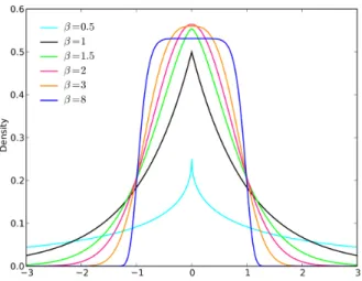
Recently alternative techniques have been reported in the literature to resolve the Gaussian assumption limitation. The generalized Gaussian distribution (GGD) has been proposed to provide more flexibility, by introducing a new parameter called the shape parameter. The GGD has three special cases concerning the varying shape parameter namely the Laplacian, the Gaussian, and the asymptotically uniform dis-tributions and can be observed in Fig. 1 where β in the figure represents the shape parameter and when β = 2, the GGD becomes Gaussian.

For instance, generalized Gaussian mixture model (GGMM) has been used in [3] for buffer control, in [4, 5, 6] for texture classification and retrieval, in [7, 8, 9] for video and image segmentation, in [10] for multiresolution transmission of high-definition video, in [11] for SAR images statistics modelling, in [12] for subband decomposition of video, in [13] for denoising applications, in [14, 15] for data and image compression, in [16] for edge modeling, in [17, 18] for image thresholding, in [19, 20] to fit subband

Figure 1: Generalized Gaussian distribution

histograms, in [21, 22] for speech modeling, and in [23] for multichannel audioresyn-thesis. The accurate modeling of wavelet coefficients distributions by GGMM was presented in [24] [25] and this property had been utilized in many signal and image processing applications which include image denoising [26], image thresholding [27], content-based image retrieval [28] and texture classification [29].

Several methods have been proposed to estimate the parameters of GGMM such as entropy matching estimation [22, 30] and maximum likelihood estimation [4, 31, 32, 33, 34] with a deterministic approach where a single distribution is considered. Maximum likelihood estimation is performed via the Expectation Maximization (EM) algorithm which has gained attention in recent times with its lower computational time. However, the EM algorithm is known for its convergence to local maxima and the tendency to overfit the model.

Solutions that incorporate Bayesian inference techniques are widely discussed in approximating intractable distributions [35]. It gives a robust hypothetical frame-work to utilize clustering algorithms. Markov Chain Monte Carlo (MCMC) is one of the most common techniques to estimate parameters since it is capable of accurately approximating the actual variable distribution [35] [36]. However, MCMC techniques are based on sampling to approximate the ideal distribution. This requires a large amount of computational time and resources [37]. Thus, in this thesis, we utilize

variational inference approaches [38]. Variational inference, also known as variational Bayes, is a deterministic approximation method, where, the model’s posterior distri-bution is approximated using analytical procedures [39]. It has recently generated more interest in finite mixture models through the provision of high generalization schemes and high computation tractability. Model selection and parameter estimation can be performed simultaneously through the use of variational inference.

Model selection plays a challenging role while applying finite mixture models with a potentially inaccurate number of mixture components may result in poor gener-alization capability. Recent studies have tackled the problem of number of mixture components by considering a Dirichlet process (DP) prior to extend mixture models to infinity [40]. The DP permits unbounded development of the number of mixture components where it is important to fit the observations, in which the individual variables follow certain parametric distributions.

Feature selection is an important step when data are multidimensional; some features could be irrelevant and then compromise the algorithm performance as well as the clustering process. Indeed, these features do not have any discriminatory impact on the clustering. Moreover, having a high number of features increases the complexity of the model [41][42]. Thus, it is important to detect the salient features to produce efficient out comes. Consequently, in this thesis we propose a DP mixture of GGD’s and employ the model proposed in [43], a feature saliency determination process, where each feature is weighted up to a probability ranging between zero and one and incorporate it into the proposed Bayesian framework.

A good alternative to DP is the Pitman-Yor process (PYP) which is a general-ization to the DP prior for nonparametric Bayesian modeling. Hierarchical Bayesian nonparametric models, during the recent years, have been successfully applied in different fields such as image segmentation and language modelling [44]. The hier-archical Dirichlet process (HDP) model has shown promising results in addressing model-based clustering of grouped data with sharing clusters [45]. Using the hier-archical Pitman-Yor (HPY) process model [46], we develop a variational learning algorithm on the resulting model to estimate the parameters and apply the proposed model for background subtraction application.

1.1

Contribution

The major contributions of this thesis are as follows:

• Variational Inference of Finite Generalized Gaussian Mixture Mod-els:

We present a variational learning framework to analyze finite generalized Gaus-sian mixture models (GGMM). The model incorporates several mixtures that are widely used in signal and image processing applications. We present a method to evaluate the posterior distribution and Bayes estimators using the variational expectation-maximization algorithm. The effective number of com-ponents of the GGMM is determined automatically. This work has been ac-cepted and published by Symposium Series on Computational Intelligence IEEE SSCI 2019 [47].

• Variational Inference of Infinite Generalized Gaussian Mixture Mod-els with Feature Selection:

We present a variational learning framework for the infinite generalized Gaus-sian mixture (IGGM) model. Infinite model addresses the model selection prob-lem; i.e., determination of the number of clusters without recourse to the clas-sical selection criteria such that the number of mixture components increases automatically to best model available data accordingly. We also incorporate feature selection to consider the features that are most appropriate in con-structing an approximate model in terms of clustering accuracy. This work has been submitted to 2020 IEEE International Conference on Systems, Man and Cybernetics (SMC) [48].

• Background Subtraction with a Hierarchical Pitman-Yor Process Mix-ture Model of Generalized Gaussian Distributions:

We present hierarchical Pitman-Yor process mixture of generalized Gaussian distributions for background subtraction. The Pitman-Yor process is integrated into our proposed model for an infinite extension that leads to better perfor-mance in the task of background subtraction. This work has been submitted to IEEE International Conference on Information Reuse and Integration (IRI 2020) [49].

1.2

Thesis Overview

The rest of this thesis is organized as follows:

• In chapter 2, we introduce variational inference for finite generalized Gaussian mixture models and show the results of our proposed model on real applications.

• In chapter 3, we extend our finite generalized Gaussian to the infinite case using Dirichlet process and apply feature selection for medical applications and image categorization.

• In chapter 4, we propose an infinite generalized Gaussian distribution based on the hierarchical Pitman-Yor process for background subtraction application.

Chapter 2

Variational Inference of Finite

Generalized Gaussian Mixture

Models

In this chapter, in order to tackle problems related to both Bayesian and deterministic estimation, we propose a variational approach. By considering possible distributions we assign appropriate priors to the mean and the precision of GGMM. We do not assign any prior distribution to the shape parameter of the GGMM to appropriately derive closed-form expressions.

This chapter is organized as follows. In Section 2.1, we present the variational inference of GGMM. In Section 2.2, we evaluate the performance of the proposed model on several applications.

2.1

Variational Inference of the Generalized

Gaus-sian Mixture Model

2.1.1

Generalized Gaussian Mixture Model

The one-dimensional generalized Gaussian distribution for a vector X ∈ _R with parameters µ, τ, λ is defined as follows:

P(X|µ, τ, λ) = λτ 1 λ 2Γ(_λ1)e −τ|(X−µ)|λ (1)

whereτ = 1 σ r Γ(3_λ) Γ(1 λ) λ

, Γ(.) indicates the Gamma function given by Γ(z) =R₀∞pz−1_e−p_dp,

where z and p are real variables. The parameters µ, σ, λ denote the mean, standard deviation and the shape parameter, respectively. The parameter λcontrols the shape of the probability density function. The higher the value, the flatter the probability density function indicating that λ determines the decay rate of the density function. There are two special cases, when λ = 2 and λ = 1, the GGD is reduced to the Gaussian and the Laplacian distributions, respectively. If X follows a mixture of K GGDs, then P(X|Θ) = K X k=1 P(X|µk, τk, λk)πk (2) whereπk (0≤πk ≤1 and PK

k=1πk = 1) are the mixing weights andp(X|µk, τk, λk) is

the probability density function corresponding to component k. As for the sym-bol Θ = (, π), it refers to the entire set of parameters to be estimated where = (µ1, τ1, λ1, ..., µK, τK, λK) and π = (π1, ..., πK).

Considering N observations, X = (X1, X2, ..., XN), and supposing that the

num-ber of componentsK is known, the data likelihood is denoted as follows: P(X |Θ) = N Y n=1 K X k=1 P(Xn|k)πk (3)

where k= (µk, τk, λk). For each variable Xn, letZn beK-dimensional vector known

as the unobserved vector that assigns the appropriate mixture component that Xn

belongs to. Then,Znk is equal to 0 ifXn does not belong to classk and 1, otherwise.

Hence, considering Z = (Z1, Z2, ..., ZN) the complete-data likelihood is given by:

P(X |Θ, Z) = N Y n=1 K X k=1 (P(Xn|k)πk)Znk (4)

The EM algorithm allows to find the mixture parameters that maximize the complete data log-likelihood given by:

L(X, Z,Θ) = N X n=1 K X k=1 Znkln(P(Xn|k)πk) (5)

The assignment of Xn to the kth component of the mixture can be denoted as follows

[50]: ˆ Z_nkt = P t−1_(X n|tk−1)π t−1 k PK k=1Pt−1(Xn| t−1 k )π t−1 k (6)

wheretdenotes the current step. t

kandptj are the current estimates of the parameters.

A sequence of approximations to the mixture parameters Θt, for t = 0,1, ..., are produced by the EM algorithm until a convergence measure is fulfilled through the expectation and the maximization steps. The EM algorithm comprises of:

1. Initialize the mixture parameters.

2. E-step: Compute ˆZ_nkt (Eq. (6)). 3. M-step: Update the parameters using

ˆ

Θt= argmax_zΘ L(Θ, Z,X).

We note that the EM algorithm has some setbacks, like convergence to local maxima due to its dependence on initialization. A discussion on the disadvantages of the EM algorithm can be found in [51].

2.1.2

Variational Inference of the Generalized Gaussian

Mix-ture Model

In this section, we propose a variational inference approach for the GGMM within the Variational Expectation-Maximization (VEM) framework [52] [53] to accomplish the closed-form updates and automatic determination of the number of mixture compo-nents by optimizing the Kullback–Leibler (KL) divergence between the true posterior p(Z,X) and the approximate distribution q(Z) [53]. The smaller the KL divergence, the stronger the relationship between the distributions. The KL divergence is denoted by: KL(pkq) =− Z q(Z) ln{p(Z,X) q(Z) −lnp(X)}dZ =− Z q(Z) ln{p(Z,X) q(Z) }dZ+ lnp(X) (7)

In order to calculate the KL divergence, we need to calculate the evidence lnp(X). This is difficult to calculate which motivates the proposed variational inference ap-proach. Reordering Eq. (7), we get:

lnp(X) =KL(pkq) +

Z

q(Z) ln{p(Z,X)

q(Z) }dZ

| {z }

Evidence Lower Bound

Maximizing the Evidence Lower Bound (ELBO) is equivalent to minimizing the KL divergence. By applying Jensen’s inequality, the ELBO serves as a lower-bound for the log-evidence, lnp(X)≥ ELBO(q) for any q(Z), which is the approximate of the posterior. In order to maximize the ELBO, we need to choose a variational family q. The complexity of the family determines the flexibility in providing an appropriate approximation to the true posterior distribution.

We assign Normal priors for the distributions mean, and Gamma priors for the precision and shape parameters [47,48]: µk ∼ N(µ|m0, s0−1), τk ∼ G(τ|α0, β0), λk ∼

G(λ|αλ, βλ) where N(µ|m0, s−01) is the Normal distribution with mean m0 and

pre-cision s−₀1, G(τ|α0, β0) is the Gamma distribution with shape parameter α0 and rate

parameter β0, λ, µ0, s0, β0, α0 are the hyperparameters of the model. The posterior

distributions forµ, τ, λ are defined as [50]: p(µk|Z, X)∝e −(µk−µ0)2s0/2+P_Znk=1−(τk|Xn−µk|)λk p(τk|Z, X)∝α_kα0−1e−β0τkτ nj k e P Znk=1−(τk|Xn−µk|)λk p(λk|Z, X)∝λ_kαλ−1e−βλλkτ nj k λk Γ(1/λk) nj ePZnk=1−(τk|Xn−µk|)λk (9)

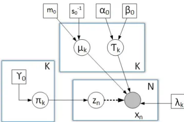
Accordingly, we can not use the posterior distributions in their current state. To formulate the variational inference model, we denote the joint distribution of all the random variables assuming all parameters are independent as can be observed in Fig. 2:

p(X, Z, π, µ, τ, λ) = p(X|Z, µ, τ, λ)p(Z|π)p(π)p(µ)p(τ)p(λ) (10)

For the shape parameter, a conjugate prior distribution can not be directly found. Therefore, we considered using the Taylor approximation to determine an approxi-mate lower bound of the complete-data log-likelihood to determine whether an ap-propriate prior exists in the exponential family. However, the negative second-order derivative causes the functionq(λ) to be concave, resulting in an upper bound rather than a lower bound; which is required. Hence, we consider λ as a parameter and it is not assigned a prior distribution [2]. The conjugate exponential priors for µand τ are Normal and Gamma distributions. Therefore, we specify all the priors according to:

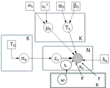
Figure 2: Graphical model for the VGGM. The filled circle, unfilled circle and square indicate observations, random variables, and parameters, respectively. The depen-dency among the variables is indicated by the arrows.

τk∼G(τ|αk, βk) (12)

We consider the following variational distribution that factorizes into the latent vari-ables and the parameters as:

q(Z, π, µ, τ, λ) =q(Z)q(π, µ, τ, λ) (13)

lnq?(Z) =_Eµ,τ,π[lnp(X, π, µ, τ, λ)] +const. (14)

lnq?(Z) =_Eπ[lnp(Z|π)] +Eµ,τ[lnp(X |Z, µ, τ, λ)] +const. (15)

where _E represents the expectation with respect to the subscripted parameter and const denotes an additive constant. Substituting the two conditional distributions, and retaining any terms that are not dependent on Z into the constant, we have:

lnq?(Z) = N X n=1 K X k=1 znklnρnk +const (16) where we define: lnρnk =Eπ[lnπk] +Eµ,τ[ 1 λk lnτk+ lnλk−ln 2Γ(1/λk) −τk|Xn−µk|λk] (17)

Normalizing the distribution, noting for each value of n the values of Znk are

binary and add up to 1 overall values of k, we obtain:

q?(Z) = N Y n=1 K Y k=1 rznk nk (18) where rnk = ρnk PK k=1ρnk (19)

The ideal solution for q(Z) follows the equivalent functional form as the prior p(Z|π). As ρnk is given by the exponential of a real quantity, the quantities ρnk will

be non-negative and will sum to one. For the discrete distribution q?_(Z):

E[znk] =rnk (20)

where rnk denotes the responsibilities with the sum of all the responsibilities for the

respective cluster k given by Nk as follows:

Nk = N

X

n=1

rnk (21)

Similarly, the factor in the variational posterior distributionq(π, µ, τ, λ) is given by:

lnq?(π, µ, τ, λ) = lnq(π) +

K

X

k=1

q(µk, τk, λk) (22)

We observe that this equation decomposes into an aggregate of terms with only π in addition to terms with µ and τ, implying that the variational posterior q(π, µ, τ, λ) factorizes to: q(π, µ, τ, λ) =q(π) K Y k=1 q(µk, τk, λk) (23)

Identifying the terms that depend on π, results in:

lnq?(π) = (γ0−1) K X k=1 lnπk+ K X k=1 N X n=1 rnklnπk+const (24)

We recognize q?(π) as a Dirichlet distribution with parameter γ:

where γ has components γk that are given by: γk =γ0+Nk (26) E[lnπk] =ψ(γk)−ψ(ˆγ) ˆ γ = K X k=1 γk (27)

The expectation of µwith prior means m0 and precision s−01 are denoted by:

E[lnq(µk)] =Eτ N X n=1 (−Znkτk|Xn−µk|λk)− s0 2(µk−m0) 2 (28)

where|Xn−µk|λk is expanded using the Binomial Expansion to the power 2 with the

following conditions: if(µk > Xn) |µk−Xn|λk =µ_kλk −λkµλ_kk−1Xn+ λk 2 (λk−1)µ λk−2 k X 2 n (29) if(Xn> µk) |Xn−µk|λk =|Xn|λk 1− µk Xn λk , 1− µk Xn λk = 1−λk µk Xn +λk 2 (λk−1) µ2 k X2 n (30)

Substituting Eq. (29) and Eq. (30) in Eq. (28) and comparing it to the prior distribution, we obtain: mk = s0m0 2 +p1 sk (31) sk = s0 2 +p2 (32)

where p1, p2 have two different cases as follows:

p1 =          PN n=1(rnk¯τkλ₄k(λk−1)µλk −3 k x 2 n+ PN n=1(rnkτ¯kλ₂kµλk −2 k xn)), if Xn< mk PN n=1rnkτ¯kλk |xn|λk xn , otherwise

p2 =          PN n=1(rnkτ¯kµ λk−2 k ), if Xn< mk PN n=1(rnkτ¯kλ₂k(λk−1) |xλkn | x2 n ), otherwise

where ¯τ represents_Eτ[τ]. Similarly, the solution for τ is as follows:

E[lnq(τk)] =Eµ λkτ 1 λk k 2Γ(_λ1 k) e−τk|X−µk|λk _{+ lnτ}α0−1 k −β0τk (33) αk= N X n=1 rnk+α0−1 (34) βk =β0 + N X n=1 rnkEµ[|Xn−µk|λk] (35) Eµ[|Xn−µk|λk] =          |Xn|λk −λk |Xn|λk Xn mk+ λk(λk−1) 2 |Xn|λk X2 n ( 1 sk +m 2 k), if Xn> µk E[|µk|λk −λkµλk −1 k Xn+ λ₂k(λk−1)µλk −2 k Xn2], otherwise

Then, using confluent hypergeometric function, _E|µk|λk can be defined as:

E|µk|λk = (√1 sk )λk _·2λk/2Γ 1+λk 2 √ π 1F1 −λk 2 , 1 2,− 1 2(mk) 2 sk . (36) The following equation denotes the lower bound:

L =_E[lnP(X |Θ)] +_E[lnP(Z|π)] +_E[lnP(π)] +_E[lnP(µ)] +_E[lnP(τ)]−_E[lnq(Z)]

−_E[lnq(π)]−_E[lnq(µ)]−_E[lnq(τ)]

(37)

The posterior distributions are obtained from the VE-step and the parameters are updated in the VM-step by augmenting the approximate lower boundL. To approxi-mate the parameters of the GGMM (i.e. λ), the first-order derivative of the estimated lower bound is set to zero, prompting:

∂L¯(q,Θ) ∂λk = ¯L0_i(q,Θ) = N X n=1 K X k=1 rnk(|Xn−µ¯k|λkln|Xn−µ¯k|(τk−τ¯k) − 1 λ2 k ln ¯τk+ 1 λk − Γ 0₍ 1 λk) 2Γ(_λ1 k) + ¯τk|Xn−µk|λkln|Xn−µk|) (38)

The second-order derivative is given by: ∂2_L¯(q,Θ) ∂2_λ k = ¯L00_i(q,Θ) = N X n=1 K X k=1 rnk(2|Xn−µ¯k|λkln|Xn−µ¯k|(τk−¯τk) + 2 λ3 k ln ¯τk− 1 λ2 k +1 2 Γ0(_λ1 k) 2 Γ(_λ1 k) 2 − Γ00(_λ1 k) 2Γ(_λ1 k) + 2¯τk|Xn−µk|λkln|Xn−µk|) (39)

The shape parameter is now estimated as:

λ?_k=λk+s∆λk where ∆λk =− L0_k(q,Θ) L00 k(q,Θ) (40)

where s is determined by the backtracking line search [54]. Our complete algorithm can then be summarized as follows:

Algorithm

1. Input: X, K, given an initial largeK value.

2. Initialization: choose α0, β0, γ0, m0, s0 using K-means algorithm, λk = 2

3. Compute αk, βk, γk, mk, sk ←Initial values for each component.

4. While Li− Li−1 ≤1e−9

5. Compute lnρnk using Eq. (60)

6. Generate the responsibilities rnk from Eq. (61)

7. Updateαk, βk, γk ← from Eq. (70), Eq. (71) and Eq. (26)

8. Calculate mk, sk from Eq. (65), Eq. (66)

9. Choose the step size s by the backtracking line search

10. Updateλk using Eq. (96)

12. Assign the cluster labels to the highest responsibilities in each row of the responsibility matrix.

13. end

2.2

Experimental results and discussion

2.2.1

Implementation details

In this section, we will be discussing about the implementation details of the pro-posed algorithm. The hyperparameters are set as α0 = µ2/σ, β0 = µ/N, given N

observations. λ = 2, m0, s−01, γ0 are initialized using K-means algorithm. Based on

these initializations, we estimate the sample mean, sample precision, and shape in the ith initial class. When the VEM algorithm stops, αk, βk, γk, mk, sk, λk are

acknowl-edged as the hyperparameter and parameter estimates in the Variational GGMM (VGGMM).

2.2.2

Dataset validation

This section has two main objectives: first applying the algorithm to estimate the mixture parameters and comparing with Variational GMM (VGMM). To reach the first objective, we apply our VGGMM estimation algorithm for binary classification in medical and astrological applications involving detection of heart diseases1 _and

predicting a Pulsar Star2 _{and finally we apply our model in image segmentation.}

Among the two data sets, the heart disease data set provides all the potential symptoms of a person having heart disease. This data set contains 76 features, however, all circulated tests allude to utilizing a subset of 14. The target field suggests the presence of heart infection within the patient. The second data set contains an example of pulsar candidates accumulated through the High Time Resolution Universe Survey. Pulsars are a phenomenal kind of Neutron star that produces radio outflow perceptible here on earth. It has picked up prominence over late occasions to mark the pulsar contender to encourage fast examination. Treating the pulsar data

1_{https://www.kaggle.com/ronitf/heart-disease-uci.}

2

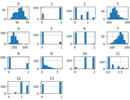
Figure 3: Histograms of Heart Disease. Histogram-0 to Histogram-12 represent the features, Histogram-13 represents the target value. X-axis indicating value range and Y-axis showing the frequency.

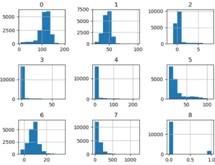
set as a binary classification problem makes it an ideal fit for our examination. The histograms of the input data sets are presented in Fig. 3 and Fig. 4.

We have implemented our VGGMM classifier using cross-validation with the split size of 4 for both the datasets. In order to determine the class-label of all the data points, the largest component is considered amongst the likelihood of the data points belonging to the classes. Table 1, presents the model accuracy in comparison with VGMM.

Table 1: Model accuracy comparison

Accuracy

Data set name VGMM VGGMM GMM

Heart Disease UCI 41% 69.64% 52% Predicting a Pulsar star 88% 93.2% 87%

Figure 4: Histograms of Pulsar Star. Histogram-0 to Histogram-7 represent the features, Histogram-8 represents the target value. X-axis indicating value range and Y-axis showing the frequency.

2.2.3

Image Segmentation

In computer vision, image segmentation is the process of finding the pixels with similar characteristics and clustering them to different segments. The goal of segmentation is to find similar pixels and represent the whole image in the form of segments with each segment representing pixels with similar characteristics making it easier for analysis [55][56].

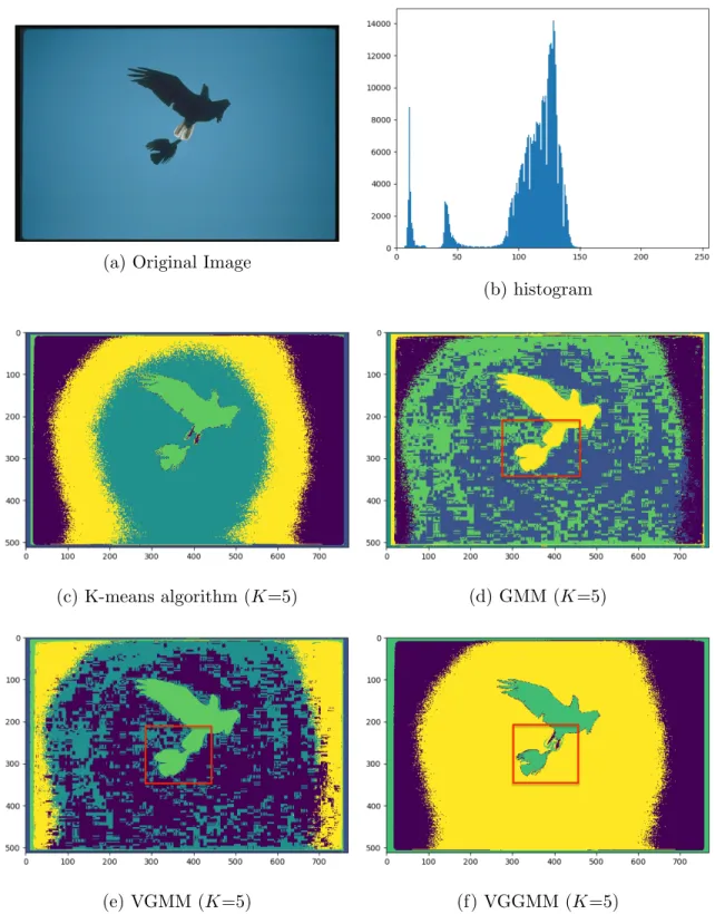
In the first experiment, we choose an image (768 x 512) with two objects in the sky to demonstrate the capability of segmenting small objects in large background (Fig. 4a). The goal is to cluster the image into two classes: the sky and the two birds. We set the number of components, K = 5. Comparing the outcomes for K-means algorithm, GMM, and VGMM (Fig. 4c, Fig. 4d, Fig. 4e), there is an enormous misclassification of the sky and the space between the little object and the large object. Our method, VGGMM (Fig. 4f), is able to recognize the two birds and the components effectively. Contrasted to the other methods, the wings, the tail of the little bird (red square), and the big bird are also shown in more details.

(a) Original Image

(b) histogram

(c) K-means algorithm (K=5) (d) GMM (K=5)

(e) VGMM (K=5) (f) VGGMM (K=5) Figure 5: Segmentation results, Fig. 4a represents the original image.

(a) Original Image _{(b) histogram}

(c) K-means algorithm (K=2) (d) GMM (K=2)

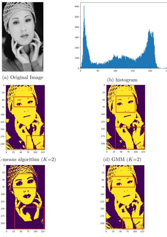
(e) VGMM (K=2) (f) VGGMM (K=2) Figure 6: Segmentation results, Fig. 5a represents the original image.

x 221) as shown in Fig. 5a to segment the image into two classes. In Fig. 5b, we can see the histogram of the image. We set the number of mixture components to two,K = 2. Comparing the result with K-means algorithm, GMM, VGMM methods, we noticed that K-means algorithm and GMM have similar results and were able to detect some features of the face. However, they contained only a part of the eyebrows and a part of the texture of clothes rather than the whole. VGMM was able to detect the eyebrows but was not able to detect the texture and the hair. Our algorithm VGGMM (Fig. 5f), was able to extract more information for image understanding.

Chapter 3

Variational Inference of Infinite

Generalized Gaussian Mixture

Models with Feature Selection

In this chapter, we develop a non-parametric Bayesian approach for modelling, par-ticularly based on the Dirichlet process (DP). Here, we employ the model proposed in [43], a feature saliency determination process, where each feature is weighted up to a probability ranging between zero and one and incorporates it into the proposed Bayesian framework.

This chapter is organized as follows. In Section 3.1, we introduce the DP and stick-breaking construction. We also introduce the simultaneous clustering and fea-ture selection algorithm and details of the proposed variational inference method. Experimental results are presented in Section 3.2.

3.1

Proposed Model

3.1.1

Dirichlet process with a stick-breaking representation

The DP is a random process with a base distributionG0 which has probability

distri-bution as its realization [57] and non-negative scaling parameterα. For DP construc-tion, a random measure G∼DP(α, G0) is drawn fromk-components of measure sets

{P1, ..., Pk} which are discrete [58]:

(G(P1), ..., G(Pk))∼(αG0(P1), ..., αG0(Pk)) (41)

The learning approach is normally based on the stick-breaking process using vari-ational inference [57]. An approximate posterior is placed on the represented set of latent variables [59]. The stick-breaking process is a representation of the DP which depends on two infinite groupings of independent and identically distributed ran-dom variables Vk and ck, for k ∈ {1, ...,∞} [60]. Using this construction, an infinite

mixture model is formed as:

p(Vk|α) = Beta(1, α) p(c∗k|α, G0)∼G0 (42)

where Vk is the stick-breaking length with concentration parameter α. c∗k represent

the atoms drawn from the base distribution G0 independently. We define the

stick-breaking representation of the random representation Gas follows: πk =Vj k−1 Y s=1 (1−Vs) G= ∞ X k=1 πkδc∗ j (43)

δc∗ is the probability concentration at c∗ with weight π. The mixing weights π = (πk)∞k=1 are formed by breaking a unit length stick into infinite pieces with weights

summing to one. Thus, the resultant has an unknown number of components that can increase as new data are observed. Thus, we have a set of observationsx={x1, ..., xN}

with parameters c = {c1, ..., cN}, where N is the total number of samples. The

distribution of random measureG is formed as follows: G|{α, G0} ∼DP(α, G0)

cn|G∼G

xn|cn∼p(xn|cn)

(44)

where G is a random measure from a DP prior DP(α, G0) and the atom cn is

in-dependently drawn from G0 with weight πn given by the nth stick-breaking length

Vn.

We utilize the above DP mixture model with the stick-breaking process. The arbitrary variable cn takes on c∗k with weight πk and the component assignment is

indicated by the latent indicator variable Zn representing the assignment of data

point xn. The generative process of the DP mixture model can be explained as

• Step 1: Vk|α ∼Beta(1, α), k ∈ {1, ...,∞}

• Step 2: c∗_k|G0 ∼G0, k ∈ {1, ...,∞}

• Step 3: Draw the nth _{observation, n∈ {1, ..., N}}

– Zn|V ∼M ulti(π)

– xn|Zn∼p(xn|c∗Zn)

From the above algorithm, the relative prevalence of the mixture is specified by the probability distribution of atomscwhich is drawn from the base distributionG0 with

stick lengths V. For the observations in Step 3, the indicators Z are distributed according to a Multinomial distribution with mixing weights π generated fromV.

3.1.2

Infinite generalized Gaussian mixture model

In this section we build an infinite generalized Gaussian mixture model (IGGM) utilizing the DP with the stick-breaking representation described in Section 4.1.1. In this thesis, we confine the proposed distribution to generalized Gaussian distribution (GGD) with set of parametersθ. We set a truncation level on the highest component number K of the stick-breaking representation. Given a dataset X ={X1, ..., XN},

if each vector Xn = (Xn1, ..., XnD) is represented in a D−dimensional space, the

truncated DP mixture model is given as follows:

p(X|Θ) = N Y n=1 K X k=1 πkp(Xn|θk) (45)

where Θ = (π1, ..., πK, θ1, ..., θK) represents the complete set of parameters for the

mixture model. π = (π1, ..., πK) represents the mixing proportions which are always

positive and sum up to one, and θk = (µk, τk, λk) represents the parameters of the

GGD for mixture componentsk. The mixing weightsπof the stick-breaking approach are represented as stick lengths V.

Given GGD parameters mean (µk), precision (τk) and shape (λk) for mixture

component k, the GGD probability density function can be written as:

P(Xn|θk)∝ D Y i=1 λikτ 1 λik ik 2Γ(_λ1 ik) e−τik|(Xni−µik)|λik (46)

where τik = 1 σik r Γ( 3 λik) Γ( 1 λik) λik

, Γ(.) denotes the gamma function given by Γ(z) =

R∞

0 p

z−1_e−p_{dp where z and p are real variables, µ}

k = (µ1k, ..., µDk), τk = (τ1k,...,τDk),

and λk = (λ1k, ..., λDk). The shape of the probability density function is determined

by the shape parameter λ. The larger the value, the flatter the probability density function. This means that the decay rate of the density function is determined by λ. Note that for the two special cases, when λ = 2 and λ = 1, the GGD is reduced to Gaussian and Laplacian distributions, respectively. In this thesis, we assume that the covariance matrix is diagonal and each dimension of observation Xn is independent

from the other dimensions.

For each variable Xn, letZn be aK-dimensional vector known by the unobserved

vector that assigns the appropriate mixture component Xn belongs to. Then, Znk

is equal to 1 if Xn belongs to class k and 0 otherwise. Hence, the complete-data

likelihood is given as follows:

P(X|Z,Θ) =

N

Y

n=1

(p(Xn|θk))Znk (47)

The mixing proportionπk =p(Znk = 1), k={1, ..., K} indicates the probability that

a data point Xn is allocated to componentk. Hence, the marginal distribution over

Z given a multinomial prior is given as follows:

p(Z|π)∼M ulti(π) = N Y n=1 K Y k=1 πI(Zn=k) j (48)

whereI(Zn=k) represents the indicator function. According to Eq. (48), the mixing

proportions π are represented by sticks V. Rearranging Eq. (48) gives p(Z|V) as follows: p(Z|V) = N Y n=1 K Y k=1 [Vk k−1 Y s=1 (1−Vs)]I(Zn=k) (49)

We truncate the number of mixture components toK, with the Beta prior of stickV from Eq. (42) p(V|α) = K Y k=1 Beta(1, α) = K Y j=1 α(1−Vk)α−1 (50)

3.1.3

Infinite generalized Gaussian mixture model with

fea-ture selection

Feature selection is an essential process in a mixture model as some features in the data do not necessarily contain information that is essential to clustering. We expect that each mixture component density is factorized over the features. Hence, the features are considered to be independent for each mixture component and we assume that a feature relevancy corresponds to a weight ranging between 0 and 1.

Thus, for each mixture component, we assume that a feature of X is drawn from a mixture of two univariate components, as proposed in [42]. The first sub-component models relevant information since it is distinctive from all other mixture components and the second sub-component represents the ”noisy” information which is common to all mixture components. Hence, we model the features with the follow-ing distribution: p(X|Z,Θ, ζ, S) = N Y n=1 K Y k=1 d Y i=1 p(Xi|Θik)snp(Xi|ζik)1−sn znk where Θ ={µ, τ, λ}, ζ ={, δ,Ω} (51) p(X, Z, π, µ, τ, λ, , δ,Ω, S) = N Y n=1 K Y k=1 d Y i=1 p(Xi|Znk, µik, τik, λik)s n i p(Xi|Znk, ik, δik,Ωik)1 −sn i (52)

where , δ, and Ω are the set of parameters for the irrelevant subcomponent. The saliency of the features is expressed through the hidden variables sn

i, where sni ∈

{0,1}. If the value of sn_i is one, then the ith feature of Xn is generated from the

relevant subcomponent; otherwise, it is generated from the irrelevant subcomponent. The distribution of the hidden variable S given the probabilities w = {wi} (feature

saliencies) is given as follows:

p(S|w) = N Y n=1 d Y i=1 ws n i i (1−wi)1−s n i (53)

3.1.4

Variational learning

In this section, we propose a variational inference framework [52] [53] for the param-eters estimation of the IGGM with feature selection. Fig. 7 represents the graphical representation of our model.

Figure 7: Graphical model for the Variational IGGM with feature selection. Filled cir-cle, unfilled circles and squares represent observations, random variables, and param-eters, respectively. The dependency among the variables is represented by directional arrows.

As discussed in the previous chapter 2 regarding the concept of variational infer-ence, the variational distribution then factorizes into the latent variables and param-eters as follows: q(V, Z, µ, τ, λ, S) = K Y k=1 q(Vk) N Y n=1 q(Zn) K Y k=1 d Y i=1 q(µik)q(τik)q(λik)q(Sin) (54)

where a Beta prior with parameters γ1 and γ2 is assigned to q(Vk), q(µik) is given a

normal prior with mean mik and precision sik and q(τik) is assigned a gamma prior

with parametersαik and βik. q(Sin) is assigned a Bernoulli prior with parameter ηin.

derivative of the functionλ is negative making the function concave [47]. q?(V) = Beta(γk1, γk2) (55) q?(µ) = N(µik|mik, s−ik1) (56) q?(τ) = G(τik|αik, βik) (57) q?(S) = ηsni in(1−ηin)1−s n i (58)

Hence, the ELBO for the proposed IGGM using the mean field assumption is given as follows: L= N X n=1 (_E[lnp(Xn|Θ)] +E[lnp(Zn)]) +_E[lnp(µ)] +_E[lnp(τ)] +_E[lnp(S)] +_E[lnp(V)] −_E[lnq(V, Z, µ, τ, λ, S)] (59)

By applying Eq. (54) for every factor, the optimal solution of the variational posterior for all the factors is given as follows:

lnρnk =EV[lnVk] + k−1 X m=1 EV[ln(1−Vm)] +Eµ,τ,s snk ln λkτ 1 λk k 2Γ(_λ1 k) −τk|X−µk|λk + (1−snk) ln kΛ 1 δk k 2Γ(1 k) −Λk|Xn−δk|k (60)

The variational parametersrnk,γ1,γ2,mik, s−ik1,αik,βik andηin are obtained by

max-imizing and determining the densities involved in q. The variational parameters are defined using the expected values ofznk, µik, τik, sni, Vk and corresponding functions of

these parameters. The following equations are obtained after deriving the expectation fromq?(V), q?(µ), q?(τ) and q?(S) as follows:

rnk = ρnk PK k=1ρnk (61) Nk= N X n=1 rnk (62) γk1 = 1 + N X n=1 rnk (63) γk2 =α+ N X n=1 K X m=k+1 rnm (64) mik = s0m0 2 +t1 sik (65) sik = s0 2 +t2 (66) ηin = wiηˆin wiηˆin+ (1−wi)εin (67) ˆ ηin = exp 1 2 K X k=1 rnk[ψ(αik)−logβik] − 1 2 K X k=1 rnk αki βki [(xn_i −mik)2+τik] (68) εin = exp − 1 2γi(x n i −i)2+ 1 2logγi (69)

where t1, t2 have two different cases as follows:

t1 =                PN n=1(rnks¯n¯τikλ₄ik(λik−1)µλik −3 ik x 2 n+ PN n=1(rnks¯n¯τik λk 2 µ λk−2 ik xn)),if Xn < mk PN n=1rnks¯nτ¯kλk |xn|λk xn ,otherwise t2 =          PN n=1(rnks¯n¯τikµ λik−2 ik ),if Xn < mik PN n=1(rnks¯nτ¯ikλ₂ik(λik−1) |xλikn | x2 n ),otherwise

where ¯τ represents _Eτ[τ]. αik = N X n=1 ¯ snrnk +α0−1 (70) βik =β0+ N X n=1 ¯ snrnkEµ[|Xn−µik|λik] (71) Eµ[|Xn−µik|λik] =                              |Xn|λik −λik |Xn|λik Xn mik+ λik(λik−1) 2 |Xn|λik X2 n ( 1 sik +m 2 ik), if Xn > µik E[|µik|λik −λikµλvik−1Xn+ λik 2 (λik−1)µ λik−2 ik Xn2],otherwise

Then using the confluent hypergeometric function results in:

E|µik|λik = (√1 sik )λik _·2λik/2Γ 1+λik 2 √ π 1 F1 −λik 2 , 1 2,− 1 2(mik) 2 sik . (72) E[lnVk] =ψ(γk,1)−ψ(γk,1+γk,2) E[ln(1−Vk)] = ψ(γk,2)−ψ(γk,1+γk,2) (73)

After the maximization of lowerbound L with respect to Q, the second step of the method requires maximization of Lwith respect towi,i, andγi. Setting the

deriva-tive ofL with respect to the parameters equal to zero results in the following update rules: wi = 1 N N X n=1 ηin (74) i = PN n=1ηinxni PN n=1ηin (75) 1 γi = PN n=1ηin(xni −i)2 PN n=1ηin (76)

Given the posterior distributions from the variational expectation (E)-step, the vari-ational maximization (M)- step updates the parameters by maximizing the approxi-mate lower bound L. To estimate the parameters of the GGD, i.e. λ,

λ?_ik =λik+ι∆λik where ∆λik =− L0_ik(q,Θ) L00 ik(q,Θ) (77)

where ι is determined by the backtracking line search [54].

Algorithm 1 Variational learning of infinite generalized Gaussian mixture model with feature selection

1. Initialization: Initialize the truncation levelK and hyperparameters αi0, βi0,

mi0,si0 and rnk using K-means algorithm, λik = 2.

2. Initialize, sn

i, wi,i,γi and ηin and compute αik, βik, mik and sik.

3. loop

i Update the irrelevant assignments wi, i, γi, and ηin from the posteriors

using Eq. (74), Eq. (75) Eq. (76), Eq. (67) and Eq. (96). ii Calculate mik and sik from Eq. (65) and Eq. (66).

iii Choose the step sizeιby the backtracking line search and updateλik using

Eq. (96).

iv The convergence criteria is reached when the difference of the current value of joint posteriors and the previous value is less than 1e−9. Otherwise, repeat above loop until convergence.

end

4. Compute the expected value of stick length Vj and the value of mixing

propor-tions using Eq. (43).

5. Detect the ideal number of mixture components K by eliminating the compo-nents with small mixing coefficients close to zero.

3.2

Experimental results and discussion

In this section, we evaluate the proposed variational IGGM model using image cat-egorization and a medical application. We compare the effectiveness of the model

based on Gaussian mixture model (GMM) and variational Gaussian mixture model (VGMM). For efficient computation, we set Ω = 2 for the irrelevant subcomponent to be a Gaussian distribution.

3.2.1

Image categorization

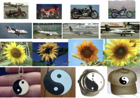
Image categorization plays an important role in automation and multimedia applica-tions where identifying patterns is vital [61]. In our experimental setup, we choose the Caltech 101 objects dataset [62]. Among the 101 categories, we choose four cat-egories: Bikes, Yin Yang, Sunflowers and Aeroplanes. All the categories have 60 images each to have a balanced dataset. Sample images are shown in Fig. 8. Also, to evaluate the robustness of our model, all the categories that are considered have a similar landscape.

Figure 8: Caltech 101 categories utilized in this chapter (top to bottom rows): Mo-torbike, Aeroplane, Sunflower, Yin Yang.

To implement our model, we initially extract features and utilize the bag of visual words (BoVW) representation [63][64]. Some of the most commonly utilized descrip-tors are Scale-Invariant Feature Transform (SIFT) [65], Speeded Up Robust Features (SURF) [66], Histogram of Oriented Gradients (HOG) [67]. In this chapter, we use SIFT features for representations of the Caltech 101 dataset. SIFT feature extraction

has the target of decreasing the subsequent computational complication and facilitat-ing credible and accurate recognition for unknown new data. Our BoVW approach consists of 200 features. Consequently, we first extract the features from the images and performK-means clustering over the extracted SIFT descriptors to form the bag of the words feature vector for each image.

Our experiments comprise of clustering with no training stage as information is infused into the algorithm with no prior knowledge about the observation labels. As outlined in Fig. 8, the Caltech 101 dataset for a given label has many number of images with different objects along with the focused object. We initialize the input dataset using K-means algorithm and start with one mixture component (K = 1). The proposed algorithm, denoted in Algorithm 1, then iterates until convergence. We evaluate the effectiveness of the model in terms of the accuracy, recall and the preci-sion metrics which are defined as accuracy = (TP + TN)/Total no of observations, recall = TP/(TP +FN) and precision = TP/(TP + FP) where TP, TN, FP, and FN represent the total number of true positives, true negatives, false positives, and false negatives respectively.

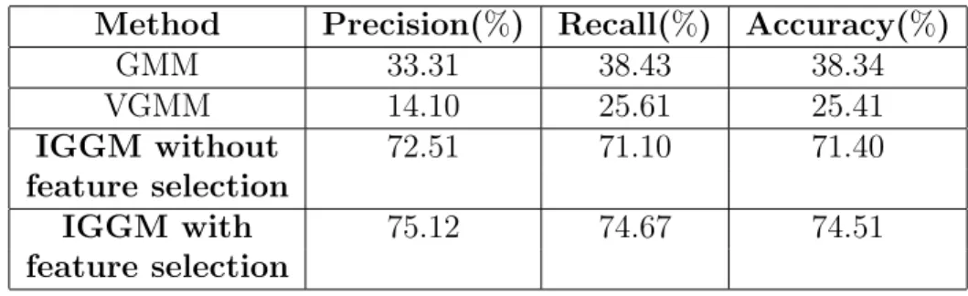
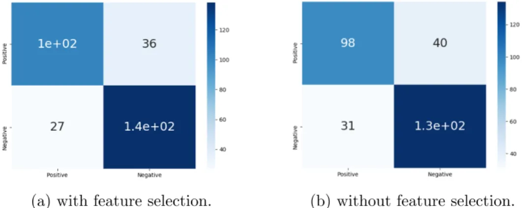
Fig. 9 depicts the confusion matrix of the variational IGGM with and without feature selection. Our results show that the model has misclassified Aeroplane as MotorBike because of the high similarity of the landscape. Nonetheless, Table 2 shows that our model outperforms the other comparing models as well as the variational IGGM without feature selection. We can observe that VGMM resulted in a much lower accuracy and precision than any other model due to overfitting. Incorporating feature selection into the IGGM has improved the accuracy by 3%.

Table 2: Results for image categorization application with the Caltech 101 dataset and 200 features.

Method Precision(%) Recall(%) Accuracy(%)

GMM 33.31 38.43 38.34 VGMM 14.10 25.61 25.41 IGGM without 72.51 71.10 71.40 feature selection IGGM with 75.12 74.67 74.51 feature selection

(a) with feature selection. (b) without feature selection. Figure 9: Confusion matrices of variational IGGM model for for Caltech 101 dataset.

(a) with feature selection. (b) without feature selection.

Figure 10: Confusion matrices of variational IGGM model for heart disease dataset.

3.2.2

Heart Disease Detection

For the second application, we apply our proposed variational IGGM estimation al-gorithm with feature selection in medical applications involving detection of heart diseases. The heart disease data set provides all the potential symptoms of a person with positive heart disease.

We have implemented our variational IGGM model with and without feature selection starting with K = 1. The label for each data point is determined with the largest component among the likelihood of the data point belonging to the classes.

Fig. 12 represents the confusion matrix results of the variational IGGM model with and without feature selection. We can observe that inclusion of feature selection increased true positives significantly by reducing the false positives when compared

Table 3: Results of Heart Disease UCI dataset.

Method Precision(%) Recall(%) Accuracy(%)

GMM 50.43 58.31 51.22 VGMM 57.07 62.31 59.10 IGGM without 77.10 77.10 76.10 feature selection IGGM with 79.33 79.34 79.33 feature selection

with the model without feature selection which is crucial in any medical-related ap-plication.

Table 3 presents the precision, recall and model accuracy of the three algorithms. Although VGMM performed better than GMM due to relatively less number of fea-tures, we can see that the variational IGGM model performed better than all the other models and the inclusion of feature selection resulted in an improvement of 3% in precision, recall and accuracy.

Chapter 4

Background Subtraction with a

Hierarchical Pitman-Yor Process

Mixture Model of Generalized

Gaussian Distributions

Gaussian mixture models (GMM) are widely used for video background subtraction [1]; however, the foreground and the background pixels are not necessarily always distributed as a Gaussian [68]. In this work, we take advantage of the flexibility of the generalized Gaussian distribution (GGD) to fit the foreground and the background pixels [47].

In this chapter, we use the hierarchical Pitman-Yor (HPY) process model [46], we develop a variational learning algorithm on the resulting model to estimate the parameters and apply the proposed model for background subtraction. The rest of the chapter is organized as follows. In the next section, we present HPY process mixture model with GGD. The model learning is presented in Section 4.2. Section 4.3 is devoted to the experimental results.

4.1

Model specification

4.1.1

Hierarchical Pitman-Yor process mixture model

The PYP for a random distribution G with a base distribution H is defined with two parameters; namely, a discount parameter ιa and a concentration parameter ιb,

satisfying 0< ιa<1, ιb >−ιa and given by [69]:

G∼P Y P(ιa, ιb, H) (78)

ιa = 0 is a special case of DP with concentration parameter ιb. The HPY process

is an extension to the PYP with a Bayesian hierarchy and the base measure is itself distributed according to a PYP prior. The HPY process consists of a base distribu-tion G0 and a group-level distribution Gj which are formed using the stick-breaking

construction. It gives an explicit representation of the HPY which depends on two infinite random variables Φ0_k = {Φ0₁, ...,Φ0_∞} and κk = {κ1, ..., κ∞} which are

inde-pendent and are distributed identically. The stick-breaking construction of the base distribution G0 can be described as follows [69]:

κk ∼H, Φ0k∼Beta (1−ιa, ιb +kιa) Φk= Φ0k k−1 Y l=1 (1−Φ0_l), G0 = ∞ X k=1 Φkδκk (79)

whereκk is the set of independent random samples distributed according to the base

distribution H. Φk represents the stick-breaking weights,

P∞

k=1Φk= 1 and δκk is an

atom atκk. The stick lengths Φ0 are defined using the two parametersιaandιb of the

Beta distribution. The stick-breaking representation of the group-level PYP process is defined as follows: ψjt ∼G0, p0jt ∼Beta (1−Ba,Bb+tBa) pjt =p0jt t−1 Y s=1 1−p0_js, Gj = ∞ X t=1 pjtδψjt (80)

where pjt represents the stick-breaking weights and satisfies

P∞

t=1pjt = 1. p0jt is

the stick-breaking lengths used to recursively cut a unit length stick into infinite number of pieces. The stick lengths p0_jt follow a Beta prior and are defined using two parameters Ba and Bb. ψjt is distributed according to the base distribution G0 and

We assign global-level indicator variables I such that Ijtk ∈ {0,1}. For each ψjt,

Ijtk = 1 if ψjt maps to the base-level atom κk which is indexed by k; Ijtk = 0,

otherwise. Hence, we can represent ψjt = κ Wjtk

k . The indicator variable follows a

Multinomial distribution with stick parameter Φ and is defined as follows:

p(I|Φ) = M Y j=1 ∞ Y t=1 Multi(Φ) = M Y j=1 ∞ Y t=1 ∞ Y k=1 ΦIjtk k (81)

As Φ is a function of Φ0 according to the stick-breaking construction in Eq. (79), we can rewrite Eq. (81) as follows:

p(I|Φ0) = M Y j=1 ∞ Y t=1 ∞ Y k=1 " Φ0_k k−1 Y l=1 (1−Φ0_l) #Ijtk (82)

The prior for Φ0 is drawn from a Beta distribution described in Eq. (79) and can be given as follows: pΦ~0= ∞ Y k=1 Γ (1−ιak+ιbk+kιak) Γ (1−ιak) Γ (ιbk+kιak) (1−Φ0_k)ιbk+kιak−1 Φ0−ιak k (83)

We construct the HPY process mixture as a factor associated with the observation Xji, where i indexes the observations within each jth group of the grouped dataset.

The HPY process mixture generates θji as a factor to every observation of Xji, and

θj = (θj1, θj2, ...) and are distributed according toGjof the PYP. Hence, the likelihood

function is given as follows:

θji|Gj ∼Gj, Xji|θji ∼F (θji) (84)

where F(θji) represent the distribution of Xji given the factor θji. The base

distri-bution H of G0 gives the prior for θji. As per this setup, each group j is related

with a mixture model, and as the atoms κk are shared among all Gj; therefore, the

mixture components are also shared among the mixture models. As each factor θji

is distributed according toGj with valuesψjt and probability pjt. We introduce one

more latent indicator variable W following the Multinomial distribution as:

p(W|p) = M Y j N Y i ∞ Y t pWjit jt (85)

Hence, for eachθji, we place an indicator variableWjit ∈ {0,1} whereWjit= 1 if θji

Therefore, we have θji = ψ Wjit

jt . Since ψjt maps to the global-level atom κk, we can

also write θji =ψ Wjit

jt =κ WjtkIjtk

k .

According to the stick-breaking construction in Eq. (80), rewriting Eq. (85) results in: p(W|p0) = M Y j N Y i ∞ Y t [p0_jt t−1 Y s=1 (1−p0_js)]Wjit ₍₈₆₎

The prior forp0 is given by a Beta distribution described in Eq. (80) and can be given as follows: p(~p0) = M Y j=1 ∞ Y t=1 Γ (1−Bajt+Bbjt+tBajt) Γ (1−Bajt) Γ (Bbjt+kBajt) 1−p0_jtBbjt+tBajt−1 p0−Bajt jt (87)

4.1.2

HPY mixture of generalized Gaussian distributions

In this thesis, we restrict the base distribution H in Eq. (78) to GGD. Given the datasetXhavingN random vectors divided intoMgroups, where eachDdimensional observation Xji = (Xji1, ..., XjiD) is drawn from a HPY process mixture model of

GGD’s with parameters µk = (µ1k, ..., µDk), τk = (τ1k,...,τDk), and λk = (λ1k, ..., λDk).

Thus, the likelihood function with the latent indicators can be given as follows [69]:

p(X|W, I, µ, τ, λ) = M Y j=1 N Y i=1 ∞ Y t=1 ∞ Y k=1

p

(

X

|

µ

, τ

, λ

)

Q

e

Γ(.) denotes the gamma function given by Γ(z) = R₀∞pz−1_e−p_{dp, where z and p are}

real variables. Normal N and Gamma G priors are assigned to the parameters µand τ with hyperparameters p, q, m, and s respectively as follows:

µkd ∼ N pkd, qkd−1

τkd ∼ G(mkd, skd)

(89)

4.2

Variational inference

In this section, we use the already presented variational inference from the previous chapter 2 to approximate a distribution q(Θ) for the true posterior p(Θ|X), where Θ ={I,Φ0, W, p0, µ, τ, λ}indicates the set of latent variables in the HPY process GGM (HPYPGGM). Thus, the mean field variational inference of HPYPGGM is given by:

q(I,Φ0, W, p0, µ, τ, λ) =q(I)q(Φ0)q(W)q(p0)q(µ)q(τ)q(λ) (90) In our algorithm, we truncate the variational approximation of the base distribution G0 at K : βK0 = 1, βk = 0 when k > K, satisfying the condition PK_k=1βk = 1.

Similarly for the variational approximate Gj at T : p0jT = 1, pjt = 0 when t >

T and, PT

t=1pjt = 1. The variational parameters K and T are optimized during

the variational learning process. Next, considering the suitable family of variational approximations, we can have the distributions for the parameters as follows:

q(I) = M Y j T Y t K Y k Multi (Ijtk|ϕjtk) q(W) = M Y j N Y i T Y t

Multi (Wjit|%jit)

q(Φ0) = K Y k Beta (Φ0_k|ck, dk) q(p0) = M Y j T Y t Beta p0_jt|ejt, fjt q(µ) = K Y k D Y d N µkd|pkd, q−kd1 q(τ) = K Y k D Y d G(τkd|mkd, skd) (91)

By applying the mean field theory for the proposed HPYPGGM, we expand the ELBO as follows:

L=Eq[logp(X|I, W, µ, τ, λ)]) +Eq[logp(I|Φ0)] +Eq[logp(Φ0|ιa, ιb)]

+Eq[logp(W|p0)] +Eq[logp(p0|Ba,Bb)]

+Eq[logp(µ|p, q−1)] +Eq[logp(τ|m, s)]

−Eq[logq(W,Φ0, I, p0, µ, τ, λ)]

where, E represents the expectation with respect to the subscripted parameter. We obtain the updated equations for the variational parameters by maximizing Eq. (92) with respect to Eq. (91) as follows:

ϕjtk = ˆ ϕjtk PK k ϕˆjtk , %jit= ˆ %jit PT t %ˆjit ˆ ϕjtk = exp ( Eq[log Φ0k] + k−1 X l=1 Eq[log (1−Φ0l)] − N X i Eq[Wjit]Re ) ˆ %jit= exp ( Eq logp0_jt+ t−1 X s=1 Eq log 1−p0_jt − K X k Eq[Ijtk]Re ) ˆ ϕjtk e R= D X d Eq[ 1 λkd logτkd−τkd|Xjid−µkd|λkd] ck= 1−γak+ M X j T X t Eq[Ijtk] dk =γbk+kγak + M X j T X t K X l=k+1 Eq[Ijtl] ejt = 1−Bajt+ N X i Eq[Wjit] fjt =Bbjt+tBajt+ N X i T X s=t+1 Eq[Wjis] mkd = M X j T X t N X i Eq[Ijtk]Eq[Wjit] +m0−1 skd = M X j T X t N X i Eq[Ijtk]Eq[Wjit] +Eq[|Xjid−µkd| λkd_{] +s} 0 pkd = p0q0 2 +t1 qkd qkd = q0 2 +t2

where m0, s0, p0 and q0 are the hyperparameters of mkd, skd, pkd and qkd. t1 and t2

are defined as:

t1 =                PM j PT t PN i (Eq[Ijtk]Eq[Wjit]Eq[τkd]λ₄kd(λkd−1)µλkd −3 kd X 2 jid+ (Eq[Ijtk]Eq[Wjit]Eq[τkd]λkd₂ µλ_kdkd−2Xjid)) ,if Xjid< pkd PM j PT t PN i Eq[Ijtk]Eq[Wjit]Eq[τkd]λkd |Xjid|λkd Xjid ,otherwise t2 =            PM j PT t PN i (Eq[Ijtk]Eq[Wjit]Eq[τkd]p λkd−2 kd ),if Xjid< pkd PM j PT t PN i (Eq[Ijtk]Eq[Wjit]Eq[τkd] λkd 2 (λkd −1) |X_jidλkd| X2 jid ),otherwise (93)

The expected values for the equations in Eq. (93) are defined as follows: Eq[Ijtk] =ϕjtk, Eq[Wjit] =%jit Eq[log Φk] =Eq[log Φ0k] + k−1 X l=1 Eq[log (1−Φ0l)] Eq[log (Φ0k)] = Ψ (ck)−Ψ (ck+dk) Eq[log (1−Φ0k)] = Ψ (dk)−Ψ (ck+dk) Eq[logpjt] =Eq logp0_jt + t−1 X s=1 Eq log 1−p0_jt Eq log p0_jt= Ψ (ejt)−Ψ (ejt+fjt) Eq log 1−p0_jt= Ψ (fjt)−Ψ (ejt+fjt) Eq[|Xjid−µkd|λkd] =                                    |Xjid|λkd−λkd |Xjid|λkd Xjid pkd+ λkd(λkd−1) 2 |Xjid|λkd X2 jid (_q1 kd +p 2 kd), if Xjid> pkd E[|µkd|λkd −λkdµλkd −1 kd Xjid+ λkd 2 (λkd−1)µ λkd−2 kd X 2 jid], otherwise (94)

defined as : Eq |µkd|λkd = (√1 qkd )λkd _·2λkd/2Γ 1+λkd 2 √ π 1F1 −λkd 2 , 1 2,− 1 2(pkd) 2 qkd (95)

The shape parameter λ is given as follows [47]: λ?_kd =λkd+υ∆λkd

where ∆λkd =−

L0_kd(q,Θ)

L00_kd(q,Θ)

(96)

where υ is determined by the backtracking line search [54].

Algorithm 2 Hierarchical Pitman-Yor process of generalized Gaussian mixture model

1. Initialization: Set the truncation levels K and T.

2. Initialize the hyperparameters ιa,ιb, Ba, Bb,p0, q0, m0 and s0.

3. Initialize %jit using K-means

4. loop

i Estimate all the expected values in Eq. (94) and Eq. (95).

ii Update the parameters of the variational solution using the equations in Eq. (93).

iii Choose the step size υ by the backtracking line search and update λkd

using Eq. (96).

iv The convergence criteria is reached when the difference between current and previous values of joint posteriors is less than 1e−9.

5. end

4.3

Experimental results and discussion

4.3.1

Background subtraction

In this section, we employ the proposed HPYPGGM to address the problem of video background subtraction using a pixel-level evaluation approach [1]. This approach classifies whether the pixel belongs to the foreground or the background. Let us con-sider a frame X containing U pixels such that X = (X~1, ..., ~XU). In the proposed

algorithm, each pixelX~i represents red, green and blue (RGB) colors (3-dimensional)

of the pixel which is modeled as a mixture of infinite GGD and the mixture com-ponents are shared between the groups (i.e., frames). The HPY process mixture

satisfies the above setting. We preprocess the frames by normalizing all the pixel values in an observed frame to unit sum. The preprocessed data is then used for learning the proposed HPYPGGM. In our mixture model, we can observe that some of the mixture components are used to model background pixels and the other mod-els the foreground pixmod-els. The final step in our framework is to determine if X~i is

a foreground or a background pixel. In the proposed model, we assume a mixture component is classified as background if it occurs frequently, indicating high Φ and high precision τ [1]. We order the estimated components according to the product of Φkτk and the resulting firstB components are classified as background components,

with B given by:

B = arg min b b X k=1 Φk >Υ (97)

where Υ represent the minimum threshold of the data that should be accounted for the background in the frame, and the other components are classified as foreground components.

4.3.2

Results and discussion

In this section, we implement the proposed HPYPGGM algorithm on the challenging Change Detection dataset [70] which consists of 31 videos categorized into 6 differ-ent categories (baseline, shadows, dynamic background, intermittdiffer-ent object motion, camera jitter, and thermal). To evaluate the efficiency of the proposed model, we consider six videos of the Change Detection dataset which are described as follows:

• Pedestrians: This video sequence shows pedestrians walking in a park.

• Office: This video sequence shows a person walking around in an office.

• Library: This thermal video sequence shows a person walking in the library.

• Corridor: This thermal video sequence shows a person walking in the corridor.

• Canoe: This video sequence shows a moving canoe in a dynamic background.

• Badminton: This video sequence shows players playing badminton.

Sample images from the videos can be found in Fig. 11. In our experiments, we initialize threshold Υ = [0.55,0.75] for different videos. Our results for each of the

(a) Pedestrians. (b) Office. (c) Library.

(d) Corridor. (e) Canoe. (f) Badminton. Figure 11: Sample frames of the video sequences from Change Detection dataset.

video sequences can be observed in confusion matrix form in Fig. 12. We evaluate the classification measure by accuracy, recall and precision which are defined as accuracy = (TP + TN)/Total no of observations, recall = TP/(TP + FN) and precision = TP/(TP + FP) where TP, TN, FP, and FN represent the total number of true positives, true negatives, false positives, and false negatives respectively. The reported results of precision and recall are based on the macro averages of the overall frames.

(a) Pedestrians. (b) Office. (c) Library.

(d) Corridor. (e) Caneo. (f) Badminton. Figure 12: Confusion matrices of applying the proposed HPYPGGM model.

We compare our results with four other approaches from the literature; namely, K-means, GMM, variational GMM (VGMM) and Dirichlet process GMM (DPGMM). We set the number of components to 6 for K-means, GMM, VGMM and DPGMM. The threshold Υ is set to the same value as HPYPGGM for a fair comparison between the models. A visual comparison of the results from all the video sequences can be observed in Fig. 13 and Table 4 shows the comparison of the proposed HPYPGGM against K-means, GMM, VGMM and DPGMM. We can observe in the Pedestrians video sequence, that our model performed better in classifying between the back-ground and foreback-ground pixels while the others misclassified most of the backback-ground with foreground pixels. In the Office video sequence, K-means, GMM, VGMM and DPGMM were not able to precisely distinguish between the background and fore-ground pixels. This may be due to the close color intensity of the person’s jeans with the color intensity of the box next to him. Nonetheless, HPYPGGM was able to segment a better foreground compared with the other models. All the models performed better in the Library video sequence where the background pixels are dark with perfect illumination, thereby resulting in a high accuracy with a supporting high precision and recall for all the models. In the Canoe video sequence all the models misclassified background water with foreground. However, HPYPGMM was able to give a better classification between the background and the foreground pixels. This can be observed clearly in Fig. 13. Similar results were obtained in the Badminton video sequence. Table 4 shows that the proposed HPYPGGM model outperformed K-means, GMM, VGMM and DPGMM in most cases in terms of precision, recall and accuracy.

Table 4: The macro average results of background subtraction with the Change De-tection dataset.

Model Precision (%) Recall (%) Accuracy (%)

Pedestrians K-means 67.30 73.11 96.48 GMM 60.12 73.42 94.02 VGMM 57.21 71.60 92.31 DPGMM 67.48 65.33 93.33 HPYPGGM 77.31 69.10 97.64 Office K-means 67.51 65.23 90.52 GMM 56.10 60.40 81.30 VGMM 58.92 65.11 81.51 DPGMM 89.48 87.12 87.21 HPYPGGM 93.31 65.20 94.05 Library K-means 98.97 96.02 98.04 GMM 98.56 96.01 98.06 VGMM 98.61 96.30 98.09 DPGMM 98.48 98.13 98.09 HPYPGGM 99.01 96.31 98.72 Corridor K-means 92.31 62.01 84.22 GMM 94.12 76.89 90.25 VGMM 95.23 78.12 83.50 DPGMM 94.48 93.21 93.01 HPYPGGM 96.01 83.51 93.43 Caneo K-means 80.10 78.26 93.22 GMM 76.82 77.12 92.59 VGMM 71.13 77.23 90.64 DPGMM 93.10 74.42 93.46 HPYPGGM 97.01 74.51 95.66 Badminton K-means 61.12 72.51 95.22 GMM 57.51 74.12 93.52 VGMM 57.12 74.71 93.50 DPGMM 66.48 65.47 94.73 HPYPGGM 66.01 66.52 97.40

Figure 13: The foreground mask results for each of the original images (Pedestrians, Office, Library, Corridor, Caneo and Badminton from top to bottom respectively) obtained by K-means, GMM, VGMM, DPGMM and HPYPGMM algorithms are shown in columns 1 to 5 respectively.