M-Quantile and expectile random effects regression for multilevel data

Working Paper M10/07

Methodology

M-Quantile And Expectile

Random Effects Regression For

Multilevel Data

N. Tzavidis, N. Salvati, M. Geraci, M. Bottai

Abstract

The analysis of hierarchically structured data is usually carried out by using random effects models. The primary goal of random effects regression is to model the expected value of the conditional distribution of an outcome variable given a set of explanatory variables while accounting for the dependence structure of hierarchical data. The expected value, however, may not offer a complete picture of this conditional distribution. In this paper we propose using linear M-quantile regression, to model other parts of the conditional distribution of the outcome variable given the covariates. The proposed random effects regression model extends M-quantile regression and can be viewed as an alternative to the quantile random effects model. Inference for estimators of the fixed and random effects parameters is discussed. The performance of the proposed methods is evaluated in a series of simulation studies. Finally, we present a case study where M-quantile and expectile random effects regression is employed for analyzing repeated measures data collected from a rotary pursuit tracking experiment.

M-quantile and Expectile Random Effects Regression for

Multilevel Data

N. Tzavidis∗ N. Salvati† M. Geraci‡ M. Bottai§

Abstract

The analysis of hierarchically structured data, for example longitudinal or geographi-cally clustered data, is usually carried out by using random effects models. The primary goal of random effects regression is to model the expected value of the conditional dis-tribution of an outcome variable given a set of explanatory variables while accounting for the dependence structure of hierarchical data. The expected value, however, may not offer a complete picture of this conditional distribution. In this paper we propose using linear M-quantile regression, to model other parts of the conditional distribu-tion of the outcome variable given the covariates, which includes random intercepts to account for the dependence of hierarchical data. The proposed random effects regres-sion model extends M-quantile regresregres-sion (Breckling and Chambers, 1988) and can be viewed as an alternative to the quantile random effects model (Geraci and Bottai, 2007). M-estimation is synonymous with outlier-robust estimation. Consequently, the proposed approach allows for robust estimation of both fixed and random effects. The proposed M-estimation framework also includes expectile regression as a special case. Expectile regression can potentially lead to efficiency gains when the use of outlier-robust estimation methods is not justified but there is still interest in modelling not only the centre but also other parts of the conditional distribution.

Fixed and random effects are estimated using maximum likelihood and inference for estimators of the fixed and random effects parameters is discussed. The performance of the proposed methods is evaluated in a series of simulation studies. Finally, we present a case study where M-quantile and expectile random effects regression is employed for analyzing repeated measures data collected from a rotary pursuit tracking experiment.

Keywords: influence function; linear mixed model; longitudinal data; M-estimation; ro-bust estimation; quantile regression; repeated measures.

1

Introduction

Linear random effects regression is widely used in the analysis of hierarchical data, such as, longitudinal or geographically clustered data (Singer and Willett, 2003; Rabe-Hesketh

∗

Social Statistics and S3RI, University of Southampton; Social Statistics and Centre for Census and Survey Research, University of Manchester, Manchester M13 9PL, [email protected]

†

Dipartimento di Statistica e Matematica Applicata all’Economia, Universit`a di Pisa, Via Ridolfi 10, Pisa 56124, [email protected]

‡

School of Cancer and Enabling Sciences, University of Manchester, Manchester M13 9PL, UK [email protected]

§

Arnold School of Public Health, University of South Carolina, 800 Sumter Street Columbia, SC 29208; Unit of Biostatistics, IMM, Karolinska Institutes, Nobels V¨ag 13, 17177 Stockholm [email protected]

and Skrondal, 2008; Goldstein, 2003). The random effects regression models a location pa-rameter, namely the expected value of the conditional distribution of an outcome variable given a set of covariates. In many situations, however, the focus of the analysis extends beyond modelling a location parameter and emphasis is also placed on modelling other parts of this conditional distribution. The idea of modelling the quantiles of a conditional distribution has a long history in statistics. The seminal paper by Koenker and Bassett (1978) is usually regarded as the first detailed development of quantile regression. This can be viewed as a generalization of median regression. In the same way, expectile regression (Newey and Powell, 1987) is a quantile-like generalization of mean regression. M-quantile regression (Breckling and Chambers, 1988) combines these two concepts within a com-mon framework defined by a quantile-like generalization of regression based on influence functions (M-regression).

Let us start with a motivating example that we will fully analyse later in this paper. Data on reaction time and hand-eye coordination were collected on 108 members of the public who visited the Human Systems Integration Laboratory at Naval Postgraduate School in Monterey, California in October 1995. One experiment that demonstrates motor learning and hand-eye coordination is rotary pursuit tracking. The subject’s task in this experiment is to maintain contact with a target spot using a metal wand. Trials were conducted for 15 seconds at a time, and the total contact time during the 15 seconds was recorded. Four trials were recorded for each subject. The age and sex of each subject were also recorded. The outcome variable is the total contact time and we are interested in investigating its association with age and sex. Two examples of research questions that we are interested in answering with this dataset are the following: (1) is the performance in motor learning and hand eye coordination affected by age and/or sex? and (2) if so, do the effects of age and/or sex depend on the level of performance itself? that is, are age and/or sex differences the same among those who perform better and those who perform worse? In analysing this dataset one must take into account its longitudinal structure and one way for doing so is by using a linear growth curve model. However, the target of a growth curve model in this case will be the expected value of the conditional distribution of contact time given the set of covariates. In this respect, a growth curve model can help in answering question 1 but not question 2. For answering question 2 we need a quantile regression model that can handle hierarchical data.

Extensions of quantile regression for modelling dependent data have been considered by Lipsitz et al. (1997), Koenker (2004), Karlsson (2008), Geraci and Bottai (2007), and Liu and Bottai (2009). More specifically, Lipsitz et al. (1997) and Karlsson (2008) propose marginal models targeting the overall trend, over subjects, for a given quantile. Koenker (2004) proposes the use of penalized quantile regression. Geraci and Bottai (2007) pro-pose a conditional model for quantile regression with random intercepts that uses the asymmetric Laplace distribution (ALD) for modelling the conditional likelihood while the distribution of the random effects is assumed to be Gaussian. Liu and Bottai (2009) fur-ther extend the conditional model by Geraci and Bottai (2007) and propose a quantile regression model with multiple random effects. The use of the ALD is mainly driven by convenience as it provides a parametric link between maximum likelihood estimation and minimizing the sum of absolute deviations.

To the best of our knowledge the existing literature on M-quantile regression can not handle dependent data. Although approaches to robust estimation in random effects models have been proposed by a series of authors (Huggins, 1993; Huggins and Loesch, 1998; Richardson and Welsh, 1995; Welsh and Richardson, 1997), these approaches focus

only on modelling a location parameter at the centre of the conditional distribution rather than the entire conditional distribution.

In this article we propose the use of a linear M-quantile random effects (random in-tercepts) regression (MQRE) model for modelling the quantiles of the conditional distri-bution of hierarchically structured data. One of the main advantages of the M-estimation framework is that it easily allows for robust estimation of both fixed and random effects. Nevertheless, robust estimation is not always justified and can potentially lead to a loss of efficiency for the model parameters. Our approach is based on the use of influence functions that depend on a tuning constant, which can be used to trade robustness for efficiency. As the value of the tuning constant tends to zero, the proposed method converges to quantile regression while as the value of the tuning constant increases, it tends to expectile regres-sion (ERE). Expectile regresregres-sion can be used to model the entire conditional distribution of interest without employing robust estimation. This feature, not available in the quantile regression offers added flexibility.

The structure of the paper is as follows. In Section 2 we revise quantile and M-quantile regression models. Section 3 reviews random effects models and focuses specifically on robust estimation. In Section 4 we present the M-quantile and expectile random effects regression models (MQRE and ERE) and discuss maximum likelihood in detail. The esti-mation algorithms are presented, approaches to inference are provided, and a small scale simulation study is employed for assessing finite sample approximations. In Section 5 we evaluate the MQRE and ERE regression models using model-based simulation studies, under a range of data generating mechanisms. We further compare MQRE and ERE to the quantile random effects model (QRRE) (Geraci and Bottai, 2007) aware of the fact that this alternative model does not target identical distributional parameters. In Section 6 we present the results from an application of MQRE and ERE to repeated measures data collected from a rotary pursuit tracking experiment. Finally, in Section 7 we conclude the paper with some final remarks.

2

Quantile/M-quantile regression

The classical regression model summarises the behaviour of the mean of a random variable

yat each point in a set of covariatesx(Mosteller and Tukey, 1977). This summary provides a rather incomplete picture, in much the same way as the mean gives an incomplete picture of a distribution. Instead, quantile regression summarises the behaviour of different parts (e.g. quantiles) of the conditional distribution ofy at each point in the set of thex’s.

In the linear case, quantile regression leads to a family of hyper-planes indexed by a real number q ∈ (0,1). For a given value of q, the corresponding model shows how the

qth quantile of the conditional distribution of y varies with x. For example, if q = 0.5 the quantile regression hyperplane shows how the median of the conditional distribution changes with x. Similarly, for q = 0.1 the quantile regression hyperplane separates the lower 10% of the conditional distribution from the remaining 90%.

Suppose (xT

i , yi), i = 1,· · · , n is an independent random sample from a population,

wherexT_i are rowp-vectors of a known design matrixXandyi is a scalar response variable

of a continuous random variable with unknown continuous cumulative distribution function

F. A linear regression model for the qth conditional quantile ofyi given xi is

Qyi(q|xi) =xi T_β

An estimate of the qth regression parameterβ_q is obtained by minimizing

n

X

i=1

[|yi−xTi βq|{(1−q)I(yi−xTiβq≤0) +qI(yi−xTi βq>0)}].

Solutions are usually obtained by linear programming methods (Koenker and D’Orey, 1987) and algorithms for fitting quantile regression are now available in standard statistical software for example, the library quantreg in R (R Development Core Team, 2004), the command qreg in Stata, and the procedure quantreg in SAS.

Quantile regression can be viewed as a generalization of median regression. In the same way, expectile regression (Newey and Powell, 1987) is a ‘quantile-like’ generalization of mean (i.e. standard) regression. M-quantile regression (Breckling and Chambers, 1988) integrates these concepts within a common framework defined by a ‘quantile-like’ general-ization of regression based on influence functions (M-regression). The M-quantile of order

q for the conditional density of y given the set of covariates x, f(y|x), is defined as the solution M Qy(q|x;ψ) of the estimating equation

R

ψq(y−M Q)f(y|x)dy = 0, where ψq

denotes an asymmetric influence function, which is the derivative of an asymmetric loss functionρq. A linear M-quantile regression modelyi givenxi is one where we assume that

M Qyi(q|xi;ψ) =xi T_β

q. (2)

That is, we allow a different set of p regression parameters for each value of q ∈ (0,1). Estimates ofβ_q are obtained by minimizing

n

X

i=1

ρq(yi−xiTβq). (3)

Different regression models can be defined as special cases of (3). In particular, using different specifications for the asymmetric loss function ρq we can obtain the expectile,

M-quantile and quantile regression models as special cases. When ρq is the square loss

function we obtain the expectile regression model if q 6= 0.5 (Newey and Powell, 1987) and the standard ordinary least squares regression if q = 0.5. When ρq is the Huber

loss function we obtain the M-quantile regression model (Breckling and Chambers, 1988). Finally, when ρq is the loss function described by Koenker and Bassett (1978) we obtain

quantile regression.

Setting the first derivative of (3) leads to the following estimating equations

n

X

i=1

ψq(riq)xi =0, (4)

where riq = yi −xTi βq, ψq(riq) = 2ψ(s−1riq){qI(riq > 0) + (1−q)I(riq ≤ 0)} and

s > 0 is a suitable estimate of scale. For example, in the case of robust regression,

s=median|riq|/0.6745. Since the focus of our paper is on M-type estimation, one may use

different influence functions such as the Huber or the Hampel influence functions. For the robust versions of our regression model, in this article we employ the Huber Proposal 2 influence function,ψ(u) =uI(−c≤u≤c) +c·sgn(u). Provided that the tuning constant

c is strictly greater than zero, estimates ofβ_q are obtained using iterative weighted least squares (IWLS). The steps of the algorithm for fitting the M-quantile regression model (2) are as follows,

1 Start with initial estimates ofβ_q ands. 2 Estimate the residualsriq.

3 Define weightswiq=ψq(riq)/riq.

4 Update the estimate ofβ_q using weighted least squares regression with weightswiq.

5 Iterate until convergence.

These steps can be implemented inRby a simple modification of the IWLS algorithm used for fitting M-regression with function rlm (Venables and Ripley, 2002, section 8.3).

The IWLS algorithm used to fit an M-quantile regression model guarantees convergence to a unique solution (Kokic et al., 1997) when a continuous monotone influence func-tion (e.g. Huber Proposal 2 with c > 0) is used. The tuning constant c can be used to trade robustness for efficiency in the M-quantile regression fit, with increasing ness/decreasing efficiency as we move towards quantile regression and decreasing robust-ness/increasing efficiency as and we move towards expectile regression. The flexibility of M-quantile regression is of particular importance for the present paper as this will allow us to also define an expectile random effects regression model.

3

Models for hierarchically structured data

Suppose we have data on an outcome variableyand a set of covariates xfornindividuals clustered withindgroups. A popular approach for modelling hierarchically structured data is to use a random effects model. In the simplest case we can define a random intercepts model

yij =xTijβ+zTjγ+ij, i= 1, ..., nj, j = 1, ...d, (5)

wherexij is a vector ofp auxiliary variables, β is ap×1 vector of regression coefficients and zj is a d×1 vector of group indicators used for defining the random part of the

model. In addition, γ denotes a d×1 vector of group-specific random effects, ij is the

individual random effect, and we assume that γ ∼ N(0, σ2_γ), ij ∼ N(0, σ2). A popular

approach for estimating the parameters of (5) is to employ maximum likelihood estimation. Assuming normality for the error components, cov(γj, γj0) = 0, forj 6=j0, and⊥γ, the

log-likelihood function is l(β, σ_γ2, σ2) =−1 2log|V| − 1 2(y−Xβ) T_V−1_{(y−Xβ), (6)}

where y is the n×1 response vector, V = Σ +ZΣγZT, Σ = σ2In, Σγ = σ_γ2Id, Z is an n×d matrix of known positive constants. Here and throughout the paper In, Id are

identity matrices of sizenand d, respectively. Estimates ofβ,γ,σ_γ2, and σ2 are obtained by solving the estimating equations obtained by differentiating the log-likelihood with respect to the parameters and setting these derivatives equal to zero (Goldstein, 2003). It is easy to see that in (6) we assume a squared loss function. In practice, however, data may contain outliers that invalidate the Gaussian assumptions. If normality is still assumed, the estimated model parameters under (6) will be biased and inefficient (Richardson and Welsh, 1995). One approach for robustifying the random effects model against departures from normality is to use an alternative loss function in the log-likelihood function that grows at slower rate than the squared loss function. This is the approach followed by Huggins (1993), Huggins and Loesch (1998), Richardson and Welsh (1995), and Welsh and Richardson (1997). In particular, robust maximum likelihood estimation for the random

effects model is performed by maximizing the following log-likelihood function

l(β, σ_γ2, σ2) =−K1

2 log|V| −ρ{V

−1/2_{(y−Xβ)}, (7)}

where ρ is a loss function, ψ is its derivate and K1 = E[εψ(ε)T] is computed over the standard normal distribution. Robust estimates ofβ,σ_γ2, andσ2 are obtained by solving the following estimating equations,

XTV−1/2ψ n V−1/2(y−Xβ) o = 0 1 2 n V−1/2(y−Xβ)oT V−1/2ZZTV−1/2ψnV−1/2(y−Xβ)o−K1 2 tr V−1ZZT = 0 1 2 n V−1/2(y−Xβ) oT V−1/2V−1/2ψ n V−1/2(y−Xβ) o −K1 2 tr V−1 = 0.

This is the maximum likelihood approach proposed by Richardson and Welsh (1995). Robust estimates of the random effects can be obtained by solving the following estimating equation with respect toγ (Fellner, 1986),

ZTΣ−1/2ψ{Σ−1/2(y−Xβ−Zγ)} −Σ−_γ1/2ψ{Σ−_γ1/2γ}=0.

An alternative estimation approach that can potentially lead to more efficient estimates of the variance components when there is a small number of groups or groups with a small number of observations is the robust restricted maximum likelihood approach proposed by Richardson and Welsh (1995) (see also Staudenmayer et al., 2009).

4

M-quantile and expectile random effects regression

With log-likelihood functions (6) and (7) we obtain respectively estimates of the parame-ters of the random effects model (5) and of its robust version. In fact, with (6) and (7) the target is respectively the expectation and a location parameter, close to the median, of the conditional distribution of the outcome variable given a set of explanatory variables. As stated in Section 2, on many occasions we are not only interested in describing the relationship between y and x near the centre of this conditional distribution, but also at other parts of the conditional distribution. In this section we propose extending the use of asymmetric loss functions in the case of hierarchically structured data.

Unlike Geraci and Bottai (2007), who assumed that the data follow an asymmetric Laplace distribution, here we remain within the M-estimation framework. Starting with (7) we note that one approach for extending the idea of asymmetric weighting of residuals in the case of hierarchical data is by defining the following modified Gaussian log-likelihood function

l(β_q, σ_γ2_q, σ2_q) =−K1q

2 log|Vq| −ρq{V

−1/2

q (y−Xβq)}, (8)

where β_q is the p×1 vector of M-quantile regression coefficients, σεq and σγq are the

quantile-specific variance components. Here ρq(u) = 2ρ(u)(qI(u > 0) + (1−q)I(u ≤ 0)

is a non-negative function and rq =V −1/2

q (y−Xβq) is a vector of scaled residuals with

componentsrijq,Vq=Σq +ZΣγqZ T_,Σ γq =σ 2 γqId,Σq =σ 2 qIn.

On closer inspection, (6) and (7) can be obtained as special cases of (8) for specific choices ofρqandq. In particular, whenq = 0.5 andρqis the square loss function we obtain

(6) whereas whenq = 0.5 and we use a loss function other than the square, for example the Huber loss function, we obtain (7). For q values other than 0.5 and for different choices of ρ the maximization of (8) will provide estimates of the fixed effects, β_q, and of the variance components, σεq, σγq, which can then be used for obtaining the MQRE or the

ERE fits. More specifically, using a square loss function in (8) at q 6= 0.5 results in an expectile random effects fit whereas using the Huber loss function in (8) results in an M-quantile random effects fit. The steps of the estimation algorithm are outlined in the next section. With function (8) we therefore extend the idea of asymmetric weighting – positive residuals are weighted by q and negative residuals by (1−q) – used in fitting the single-level M-quantile regression (Breckling and Chambers, 1988), to asymmetric weighting for obtaining a regression fit for the entire conditional distribution f(y|x) accounting at the same time for the dependence structure in hierarchical data.

One characteristic of M-quantile random effects regression is that in addition to ob-taining quantile-specific estimates of fixed effects, we now also obtain quantile-specific estimates of variance components. The easiest way of interpreting these quantile-specific variance components is by focusing on a regression model without covariates. Using a square loss function at q = 0.5, these variance components are the between and within group variance around the mean. Similarly, using an alternative loss function, e.g. the Huber one atq= 0.5, these variance components represent the between and within group variance around a location parameter that is close to the median. Forq6= 0.5 the quantile-specific variance components represent the between and within group variance around conditional locations other than the median.

4.1 Estimation algorithm

1 Start by assuming that (σ2

γq, σ

2

q) are known.

2 Given these variance components, form the covariance matrixVq, and estimate β_q

by solving

XTV_q−1/2ψq{Vq−1/2(y−Xβq)}=0 (9)

using IWLS. In this case, ˆ

β_q={(V_q−1/2X)TWV_q−1/2X}−1(V_q−1/2X)TWV_q−1/2y,

where W is the n×n matrix of weights obtained for unit i in group j as wij =

ψq(rijq)/rijq.

3 Use the estimates of β_q to obtain estimates of the variance components. The ML estimates of the variance components are obtained by maximizing (8) with respect to (σ2_γq, σ2_q). The corresponding score functions are:

1 2 n V_q−1/2(y−Xβ_q)oTV_q−1/2ZZTV_q−1/2ψq n V−_q1/2(y−Xβ_q)o −K1q 2 tr V−_q1ZZT = 0 (10) 1 2 n V−_q1/2(y−Xβ_q)oT V_q−1/2V_q−1/2ψq n V−_q1/2(y−Xβ_q)o −K1q 2 tr V−_q1 = 0. (11) For maximizing (8) we use the function constrOptim in R by supplying the log-likelihood function and the score functions.

4 Iterate steps 2 and 3 until convergence.

5 At convergence, estimates of the random effects atqth quantile fit are obtained by solving the following estimating equation with respect to γ_q

ZTΣ−_q1/2ψq{Σ−q1/2(y−Xβq−Zγq)} −Σ −1/2

γq ψq{Σ −1/2

γq γq}=0. (12)

An alternative estimation approach that includes an adjustment to allow for the loss of degrees of freedom incurred in estimating the fixed effects is the maximization of the restricted version of the modified Gaussian log-likelihood (8). It can be used when the number of groups of the number of observations within groups are small.

In practice the MQRE and ERE fits can be obtained by changing the value of the tuning constantcin the influence function. Using for example the Huber influence function, and setting this to the typical valuec= 1.345 we obtain the MQRE regression fit while setting

c equal to an arbitrary large value results in the ERE regression fit. With c equal to an arbitrary large value at q = 0.5 the ERE and the linear random effects (LRE) regression fits are equivalent.

4.2 Inference

Distribution theory for the parameters of the linear random effects model when the Gaus-sian assumptions hold has been studied by Hartley and Rao (1967) and Miller (1977). In the presence of outliers, however, the Gaussian assumptions are violated and large sample approximations are required. Huber (1967) proved consistency and asymptotic normality of maximum likelihood estimators when (i) the true distribution underlying the obser-vations does not belong to the parametric family defining the ML estimators, and (ii) the second and higher derivatives of the likelihood function are not available. The work of Huber (1967) is specifically linked to robust estimation problems and his arguments are used by Welsh and Richardson (1997) for proposing approximate inference for the robust ML estimators of the linear random effects model. Since the log-likelihood function (8) is an extension of the log-likelihood function (7), a sketch of the evaluation of the stochastic behaviour of ML estimators ˆθq = ( ˆβ

T q,σˆ2γq,σˆ

2

q)

T _{is given in this section}

us-ing the developments in Huber (1967) and Welsh and Richardson (1997). The estimators ˆ θq= ( ˆβ T q,σˆ2γq,σˆ 2 q)

T _{satisfy a set of estimating equations of the form}

d X j=1 Φqj(θq) =0, (13) whereΦqj(θq) = ΦT_qjβ q,Φqjσ2γq,Φqjσq2 T

, for particular choices of Φqj(θq). Under a

gen-eral response distributionD, the estimator ˆθq satisfying (13) is estimating a root θq of d X j=1 ED[Φqj(θq)] =0. (14) Provided that −n−1 d X j=1 ED[∂Φqj(θq)/∂θq]→G, (15)

where the (p+ 2)×(p+ 2) matrixG is positive definite, and n−1 d X j=1 ED Φqj(θq)TΦqj(θq) →F, (16)

a Taylor series approximation which holds uniformly in a neighborhood ofθq is

ˆ θq=θq+G−1n−1 d X j=1 Φqj(θq) +op(n−1/2), asn→ ∞. (17)

Under the regularity conditions described by Huber (1967), it follows that

n1/2ˆθq−θq

_D

−→N 0,G−1F(G−1)T

, asn→ ∞. (18)

The components of the information matrix G and the variance of the normalized score functions F for ML estimators are given in Appendix. The covariance matrix can be consistently estimated by ˆG−1Fˆ( ˆG−1)T where the matrices ˆGand ˆFare evaluated at ˆθq.

The variance of ˆβ_q can be also estimated following Street et al. (1988), ˆ V( ˆβ_q) = (n−p) −1Pd j=1 Pnj i=1ψq2(ˆrijq) h n−1Pd j=1 Pnj i=1ψ0q(ˆrijq) i2 (X T_Vˆ−1 q X) −1 ₍₁₉₎

where ˆrijq is the ith component of the vector ˆrq = ˆVq−1/2(y−Xβˆq), ψ2q(ˆrijq) = ˆw2_ijqrˆ_ijq2 ,

ψ0_q(ˆrijq) =

qI(0<rˆijq ≤c) + (1−q)I(c <rˆijq ≤0) and ˆwijq is the final weight in the

IWLS process. An approximate confidence interval of level (1−α) for theβ_q fixed effects is ˆ β_q±z(1−α/2) q ˆ V( ˆβ_q), (20)

wherez(1−α/2) denotes the (1−α/2) quantile of the standard normal distribution. The variance of (ˆσ2_γq,ˆσ2_q) is also obtained from (18). Following Pinheiro and Bates (2000), an approximate confidence interval of level (1−α) for the variance components at

q is obtained using ˆ σ2_γqexp ( −z(1−α/2) 1 ˆ σ2 γq n−1/2 q ˆ V(ˆσ2 γq) ) ,σˆ_γ2_qexp ( +z(1−α/2) 1 ˆ σ2 γq n−1/2 q ˆ V(ˆσ2 γq) )! (21) and ˆ σ_ε2_qexp ( −z(1−α/2) 1 ˆ σ2 εq n−1/2 q ˆ V(ˆσ2 εq) ) ,σˆ2_εqexp ( +z(1−α/2) 1 ˆ σ2 εq n−1/2 q ˆ V(ˆσ2 εq) )! . (22) An alternative approach for computing the variance of the estimated parameters and for constructing confidence intervals is by using parametric bootstrap. A recent example of using parametric bootstrap in the case of the robust random effects model is given by Sinha and Rao (2009). The drawback of using bootstrap in the case of MQRE and ERE regression is the computation time required for performing a large number of bootstrap replicates. We have performed some limited empirical assessment of the parametric bootstrap procedure and the results appear to be close to those obtained from the analytic approximations presented earlier on in this section.

4.3 Evaluating the asymptotic approximations

Before evaluating the performance of MQRE and of ERE regression, in this section we assess the large sample approximations outlined in Section 4.2. To this end, we design a small scale Monte-Carlo simulation study. Data are generated under the following location-shift model

yij = 100 + 2x1ij +γj+εij, i= 1, . . . ,4, j = 1, . . . ,100,

where the values ofx1 ∼U[0,15]. Different distributions have been considered for the error termsεij (level 1) and γj (level 2). In particular, we consider two scenarios for generating

the error terms:

[0,0] - No outliers: γ ∼N(0,16) andε∼N(0,36).

[ε, γ] - Outliers in both hierarchical levels: γ ∼ N(0,16) for j = 1, . . . ,90, and γ ∼

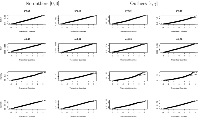
N(0,225) forj= 91, . . . ,100; ε∼δN(0,36) + (1−δ)N(0,1100) where δ ∼Bn(0.9). The tuning constantcis set to 1.345 for MQRE and to 100 for ERE. For this simulation study, we replicateR= 1000 datasets. Since we are interested in inference under the correct model, we present results only for the ERE under scenario [0,0] and results only for MQRE under scenario [ε, γ]. The complete tables are not reported here but are available from the authors upon request. To start with, Table 1 presents results on how well the variance of the fixed effects and of the variance components is estimated. For each scenario and for each estimator ˆθ, atq= 0.25 and q= 0.5, Table 1 reports

(a) The Monte-Carlo variance,

S2(ˆθ) =R−1

R

X

r=1

(ˆθ(r)−θ¯)2,

where ˆθ(r) is the estimated parameter at quantile q for the rth replication and ¯θ=

R−1PR

r=1θˆ(r).

(b) The estimated variance of ˆβ_q, ˆσ_γ2_q and ˆσ2_q averaged over the Monte-Carlo replica-tions.

(c) The coverage rate of nominal 95 per cent confidence intervals and their mean length. The coverage of these intervals is defined by the number of times the interval, defined by the estimate of the parameter plus or minus twice its estimated variance, contains the ‘true’ population parameter.

Under scenario [0,0], the asymptotic variance of the estimators of ERE at q = 0.25 and q = 0.5 provide a good approximation to the true variances. In this case, there are no outliers and hence there is no reason to employ robust estimation. Turning now to the results for scenario [ε, γ], we note that the approximation to the true variance of the estimated parameters of MQRE is overall satisfactory although there is a noticeable underestimation of the variance of the level 2 variance component. These results can potentially improve as the number of observations within groups and the number of groups increases.

We now focus on the construction of confidence intervals. Figure 1 presents normal probability plots of the estimates of the fixed effects and of the variance components under the two scenarios. Under scenario [0,0] we note that for all target parameters a normal approximation is reasonable. Under scenario [ε, γ], a normal approximation appears to be reasonable for the fixed effects and for the level 1 variance component. For the level 2 variance component there are some departures from normality but these are not very

severe. This is supported by the fact that the coverage rates of normal confidence intervals for the level 2 variance component are about 92% for bothq = 0.25 andq = 0.5.

[Table 1 about here.] [Figure 1 about here.]

5

Simulation Study

In this section we report Monte-Carlo simulation results that we carried out for assessing the performance of MQRE and ERE at two quantiles, q = 0.25 and q = 0.5. Data are generated under the following location-shift model

yij = 100 + 2x1ij+ 3x2ij+γj+εij, i= 1, . . . ,6, j= 1, . . . ,100,

where the values of x1 ∼ U[0,15], and the values of x2 are set equal to the values

x1j = 1, x2j = 2, . . . , x6j = 6, and are kept constant throughout the simulations. The

level 1 and level 2 error terms γj and εij are independently generated according to four

scenarios:

[0,0] - No outliers: ε∼N(0,36) andγ ∼N(0,16).

[ε,0] - Outliers only at the individual level (level 1):ε∼δN(0,36) + (1−δ)N(0,1100) and

γ ∼N(0,16), whereδ∼Bn(0.9).

[0, γ] - Outliers only at the group level (level 2): ε ∼ N(0,36), γ ∼ N(0,16) for j = 1, . . . ,90, andγ ∼N(0,225) forj= 91, . . . ,100.

[ε, γ] - Outliers in both hierarchical levels: error terms are generated as above but with contamination at both levels.

Each scenario is independently replicated R = 500 times. Under scenario [0,0] the as-sumptions of the random effects model (5) are valid. Scenarios [ε,0], [0, γ] and [ε, γ] define situations under which the presence of outliers is likely and hence the Gaussian assump-tions of model (5) are violated. The aim of this simulation study is two-fold. First, we assess the ability of MQRE and ERE to account for the dependence structure of hierar-chical data. Second, we compare MQRE to the quantile random effects (QRRE) model proposed by Geraci and Bottai (2007). The tuning constant c is set at the same values used for the simulation study described in Section 4.3.

Starting with the first aim, we compare the MQRE and the linear M-quantile (MQ) regression model (see Section 2), for which we also use the Huber Proposal 2 influence function withc= 1.345. Although both MQRE and MQ are robust to outliers, we expect that MQRE will perform better than the single levelM-quantile model when clustering is present. Atq = 0.5 MQRE is compared with the linear random effects (LRE) model (5). We expect that when outliers are present, MQRE will perform better than the LRE. For other quantiles we also compare the MQRE and ERE models. In this case ERE replaces LRE and we expect that when outliers are present that MQRE will be superior. For comparing the different methods we mainly focus on the fixed effects parameters. For each regression parameter performance is assessed using the following indicators:

(a) Average Relative Bias (ARB) defined as

ARB(ˆθ) =R−1 R X r=1 ˆ θ(r)−θ θ ×100,

where ˆθ(r) is the estimated parameter at quantile q for the rth replication and θ

is the corresponding ‘true’ value of this parameter. The empirical values of each parameter are computed previously with 10,000 Monte Carlo replicates to ensure better accuracy, since they are the reference values.

(b) Relative Efficiencies (EFF) defined as

EF F(ˆθ) = S 2 model(ˆθ) S_MQRE2 (ˆθ) whereS2(ˆθ) =R−1PR r=1(ˆθ(r)−θ¯)2 and ¯θ=R −1PR r=1θˆ(r).

This efficiency measure is also used for comparing estimates of the variance components obtained from the MQRE and LRE atq = 0.5 or the ERE atq = 0.25.

Table 2 reports the simulation results for estimators of the fixed effects under the different approaches. Under the scenario [0,0] and quantile q = 0.5, the estimators of the fixed effects from LRE are more efficient than the corresponding estimators from MQ. This is expected because the LRE correctly models the two level structure present in the synthetic population data. The estimators of the fixed effects of the LRE model are also more efficient than the corresponding estimators from the MQRE. Under this scenario there is no reason to employ outlier-robust estimation. Doing so results in paying a premium that is reflected in the lower efficiency of the MQRE regression estimators. At

q = 0.25, the estimators of the fixed effects of the ERE are also more efficient that the corresponding estimators of MQ and MQRE. This demonstrates the ability of the ERE to extend the LRE model for modelling other quantiles.

The superior performance of MQRE is demonstrated in scenarios [ε,0] and [ε, γ] where outliers exist either at level 1, or at both hierarchical levels. In particular, in most cases the estimators of the fixed effects from MQRE are more efficient than the corresponding estimators from MQ or from LRE/ERE. These results provide evidence that using MQRE regression protects against outlying values and it accounts for the dependence structure of hierarchical data when modelling the conditional quantiles. Finally, it appears that having outliers only at level 2 (scenario [0, γ]) does not have a severe effect on the efficiency of the estimators of the fixed effects.

Table 2 also reports the efficiency of the estimators of the variance components and the average over simulations under the four scenarios. We note that under contamination there are large gains in efficiency when using MQRE instead of ERE atq = 0.25 or LRE at

q= 0.5. In contrast to this, under the [0,0] ERE and LRE perform better than MQRE as expected. In this case the robustness offered by MQRE is unnecessary and this is reflected in the lower efficiency of the estimators of the variance components.

[Table 2 about here.]

Having assessed the performance of MQRE and ERE, in the second part of this section we wish to compare the MQRE to the QRRE model (Geraci and Bottai, 2007). A direct comparison is difficult because MQRE and ERE give M-quantile regression fits while on the other hand QRRE aims at modelling ordinary quantiles. We therefore limit our comparison to the median, the only parameter for which the two approaches are comparable. We use two indicators, the Mean Average Squared Error (MASE) and the Mean Absolute Deviation Error (MADE) respectively defined by

M ASE = (Rn)−1 n X i=1 R X r=1 (ˆy_iq(r)−y(_iqr))2 M ADE= (Rn)−1 n X i=1 R X r=1 |ˆy_iq(r)−y(_iqr)|,

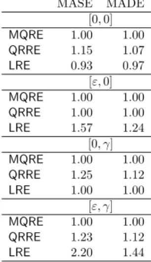
where ˆy(_iqr) is the predicted value of unitiat quantile q for the rth replication and y(_iqr) is the corresponding true value. The results of these experiments are presented in Table 3, which shows MASE and MADE expressed as ratios to, respectively, MASE and MADE obtained for MQRE. Note that at the median ERE and LRE models are equivalent. As expected, LRE works well in scenario [0,0]. In the presence of outliers, MQRE is overall performing best and also appears to perform a bit better than the QRRE. This result can be partially explained by the lack of robustness of the QRRE model to contamination of the random effects. Also, the Monte Carlo approach adopted by Geraci and Bottai (2007) for estimating the parameters of QRRE introduces additional variability to the estimation process which can affect, on some occasions, the overall convergence of the estimation algorithm. Alternative estimation algorithms based on numerical integration techniques are currently being investigated. Finally, outliers at level 2 do not appear to have a significant effect. These results indicate that in comparison to competitor models, MQRE performs very well and that both the MQRE and QRRE provide reasonable quantile random effects regression fits. As part of our empirical investigations we have also produced results for the penalized quantile regression model (Koenker, 2004). These results are not reported here, but in line with Geraci and Bottai (2007) we also find that the QRRE model performs better than the penalized quantile regression model.

[Table 3 about here.]

6

A Case Study: Analysis of rotary pursuit tracking

exper-iment data

Discovery Day is a day set aside by the United States Naval Postgraduate School in Monterey, California, to invite the general public into its laboratories. On Discovery Day, 21 October 1995, data on reaction time and hand-eye coordination were collected on 108 members of the public who visited the Human Systems Integration Laboratory. One experiment that demonstrates motor learning and hand-eye coordination is rotary pursuit tracking. The equipment used has a rotating disk with a 3/4 inches target spot. The subject’s task is to maintain contact with the target spot with a metal wand. The target spot on the circle tracker keeps constant speed in a circular path. The target spot on the box tracker has varying speeds as it traverses the box, making the task potentially more difficult. Trials were conducted for 15 seconds at a time, and the total contact time during the 15 seconds was recorded. Four trials were recorded for each of 108 subjects thus giving n = 432 observations in all. The age and sex of each subject were also recorded. The outcome variable is the total contact time and we are interested in investigating its association with age, sex, and shape.

Having each trial been recorded for all individuals, measurements of different trials pertaining the same subject could be, in general, correlated. Therefore, appropriate meth-ods that account for the dependence structure in the data must be employed. Ignoring the

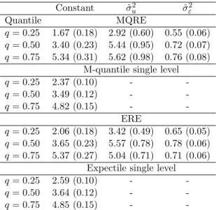
longitudinal structure, in fact, could lead to misleading results. We assess how this would impact on our analysis by estimating the following simplified regressions (intercept-only models): (a) MQRE regression (c= 1.345), (b) ERE regression (c= 100), (c) a single level M-quantile regression (c = 1.345), and (d) a single level expectile regression (c = 100). MQRE and ERE include subject-specific random effects (random intercepts) while the single level regression models ignore the fact that for each subject we have repeated obser-vations. The results are reported in Table 4. We see that failing to account for the repeated measures design has an impact on the variance of the intercept term. In particular, the variance of the intercept terms of the single level regression models is notably smaller than the corresponding variance of MQRE and ERE. The results for ERE atq = 0.5 are identical to those produced by the lme function in R and the results of the single level expectile regression at q = 0.5 are identical to those produced by functionlm in R. This confirms that our algorithm reproduces the results of standard software.

[Table 4 about here.]

We now analyse the data by estimating MQRE and ERE regression fits at q ∈ {0.25,0.5,0.75}. In the fixed part of the linear predictor we include trial, sex (female=1, male=0), age group (2 to 8, 9 to 11, 12 to 28, 29 to 38 and 39 to 52 years) of the individuals and an indicator variable for the shape of the tracker (box=1, circle=0). The random part is defined by a subject-specific intercept. Estimation is performed by using the maximum likelihood estimation approach (see Section 4.1) and the Huber Proposal 2 influence func-tion withc= 1.345 (MQRE) andc= 100 (ERE). The results are reported in Table 5 and Figure 2. Figure 2 shows box-plots of the observed contact time for females and males. In addition, it plots the estimated quantile lines of the contact time by age group for males and females and for the different shapes of tracker by averaging the predictions under the different M-quantile and expectile fits over trials.

Examining Figure 2, we detect the asymmetry of the distribution of contact time, since the estimated quantile lines at q = 0.25 and q = 0.5 are closer than the estimated quantile lines at q = 0.5 and q = 0.75. The positive asymmetry can be also observed in the fixed effects estimates reported in Table 5. The estimated intercept at q= 0.5 is 1.49 for the MQRE and 1.57 for ERE. These two numbers are respectively estimates of the median and mean of contact time at the first trial for the reference subject i.e. a male, in age group 2 to 8 years that uses a circle tracker. Moreover, the estimates of the between subjects variance component appear to be increasing withq with the estimates under the MQRE model being smaller than the corresponding ERE estimates, which may indicate the presence of outliers.

With MQRE and ERE we are also able to examine the impact of the different covariates across quantiles. The effect of trial is positive since subjects’ performance improves over time . In addition, the impact of trial appears to be constant across quantiles. Also, subjects who use a circle as a tracker have higher contact times than those that use a box as a tracker. Taking into account the standard errors of these estimates, the effect of shape appears to be constant across quantiles i.e. individuals with higher contact times face the same difficulties in using a box as a tracker as individuals with lower contact times. Overall, males have better contact times than females. This gender gap, also illustrated by Figure 2, appears to be more evident in the middle rather than at the top end of the distribution. In other words, the contact time is similar between the best-performing females and males. Finally, age appears to have a non-linear effect. The contact time increases until age 28, is stable between 28 and 38 years, and then decreases after 38 years (see Figure 2) with the

the positive effect of age on contact time being more pronounced at the top end rather than at the lower end of the distribution.

[Figure 2 about here.] [Table 5 about here.]

7

Discussion

In this paper we propose the extension of M-quantile and expectile regression to M-quantile and expectile random effects regression. Our proposed method combines M-quantile and expectile regression for the analysis of dependent data. It inherits robustness to outliers from the former and efficiency from the latter and permits to control directly the trade-off between the two by means of a tuning constant. As illustrated in the real-data example, the proposed approaches to modelling conditional quantiles may prove a useful alternative to current approaches to the analysis of hierarchical data. In a simulation study specifically designed to evaluate the impact of outliers on the robustness of the estimates, the proposed methods appeared to perform consistently well across all scenarios considered. One limi-tation of MQRE and ERE is that they allow for a very specific correlation structure. More specifically, in this paper we considered regression models with random intercepts, which is equivalent to assuming a uniform or exchangeable correlation structure. Although this structure may be adequate in many applications with hierarchical data, it may be unsat-isfactory for others. Future work will extend the proposed approaches for handling more complex correlation structures including random coefficient models.

Appendix

In this Appendix we derive the information matrix and the normalized score functions for obtaining the variance-covariance matrix ofθq = (βTq, σγ2q, σ

2

q)

T_{. The information matrix} Gn(θq) has components Gnβ_qβ_q(θq) =n−1 d X j=1 XT_jV−_qj1/2Ψ0_qjV−_qj1/2Xj, (A-1) with Ψ0_qj is a nj ×nj diagonal matrix with the ith component equal to 2(1−q)I(−c 6

rijq <0) + 2qI(0< rijq 6c), gnβqτkq(θq) = 1 2n d X j=1 XT_jV−_qj1/2∂Vj ∂τkq ψq n V_qj−1/2(yj−XTjβq) o +XT_jV−_qj1/2Ψ0_qjV_qj−1∂Vj ∂τkq V−_qj1/2(yj−XTjβq) (A-2) whereτq= (σγ2q, σ 2 q) T_, gnτkqτlq(θq) = 1 2n d X j=1 (3/2)nV−_qj1/2(yj−XTjβq) oT V−_qj1/2∂Vqj ∂τkq V−_qj1∂Vqj ∂τlq V−_qj1/2

ψq n V_qj−1/2(yj−XTjβq) o + (1/2)nV−_qj1/2(yj−XTjβq) oT V_qj−1/2∂Vqj ∂τkq V_qj−1/2Ψ0_qj V−_qj1∂Vqj ∂τlq V−_qj1/2(yj −XTjβq) −K1qtr V_qj−1∂Vqj ∂τkq V−_qj1∂Vqj ∂τlq , (A-3) whereGnβqβq(θq) is ap×pmatrix, gnβqτkq(θq) isp×1 vectors, andgnτkqτlq(θq) is scalar.

The matrix Gn(θq) of size (p+ 2)×(p+ 2) can be expressed as

Gn(θq) =       Gnβ_qβ_q(θq) " g_nβ qσγq2 (θq) g_nβ qσ2q(θq) # " g_nβ qσ2γq(θq) g_nβ qσq2 (θq) #T " g_nσ2 γqσγq2 (θq) gnσ2γqσ2q(θq) g_nσ2 qσ2γq(θq) gnσq2 σq2 (θq) #       . (A-4)

The variance-covariance matrixFn(θq) of the normalized score functions is

Fnβqβq(θq) =n −1 d X j=1 XT_jV−_qj1/2E ψq n V_qj−1/2(yj−XTjβq) o ψq n V−_qj1/2(yj−XTjβq) oT Ψ0_qjV−_qj1/2Xj o , (A-5) fnβ_qτ_kq(θq) = 1 2n d X j=1 XT_jV−_qj1/2E ψq n V_qj−1/2(yj −XT_jβ_q) o n V−_qj1/2(yj−XT_jβ_q) oT V_qj−1/2∂Vqj ∂τkq T V−_qj1/2ψq n V−_qj1/2(yj−XTjβq) o ) (A-6) fnτkqτlq(θq) = 1 2n d X j=1 E n V−_qj1/2(yj −XTjβq) oT V_qj−1/2∂Vqj ∂τkq V−_qj1/2ψq n V−_qj1/2(yj−XTjβq) o −K1qtr " V−_qj1∂Vqj ∂τkq T#) n V_qj−1/2(yj −XT_jβ_q) oT V−_qj1/2∂Vqj ∂τlq V−_qj1/2 ψq n V−_qj1/2(yj−XT_jβ_q) o −K1qtr V−_qj1∂Vqj ∂τlq (A-7) The matrix Fn(θq) of size (p+ 2)×(p+ 2) can be expressed as

Fn(θq) =       Fnβqβq(θq) " f_nβ qσ2γq(θq) f_nβ qσ2q(θq) # " fnβqσγq2 (θq) fnβqσ2q(θq) #T " fnσ2 γqσ2γq(θq) fnσ2γqσ2q(θq) fnσ2 qσγq2 (θq) fnσq2 σq2 (θq) #       . (A-8)

References

Breckling, J. and Chambers, R. (1988). M-quantiles. Biometrika75, 761–771.

Davis, C.S. (1991). Semi-parametric and non-parametric methods for the analysis of re-peated measurements with applications to clinical trials. Statistics in medicine, 10, 1959–1980.

Fellner, W.H. (1986). Robust Estimation of Variance Components. Technometrics, 28, 51–60.

Geraci, M. and Bottai, M. (2007). Quantile regression for longitudinal data using the asymmetric Laplace distribution. Biostatistics,8, 140–54.

Goldstein, H. (2003). Multilevel Statistical Models. Wiley, NewYork.

Hartley, H. O. and J. N. K. Rao (1967). Maximum-likelihood estimation for the mixed analysis of variance model, Biometrika,54, 93–108.

Huber, P.J. (1967). The behavior of maximum likelihood estimates under nonstandard conditionsProceedings of the Fifth Berkeley Symposium on Mathematical Statistics and Probability,1, 221–233.

Huber, P.J. (1981). Robust Statistics. John Wiley & Sons, NewYork.

Huggins, R.M. (1993). A Robust Approach to the Analysis of Repeated Measures. Bio-metrics,49, 255–268.

Huggins, R.M. and Loesch, D.Z. (1998). On the Analysis of Mixed Longitudinal Growth Data. Biometrics,54, 583–595.

Karlsson, A. (2008). Nonlinear quantile regression estimation of longitudinal data. Com-munications in Statistics - Simulation and Computation,37, 114–131.

Koenker, R. and Bassett, G. (1978). Regression quantiles. Econometrica,46, 33–55. Koenker, R. and D’Orey, V. (1987). Computing regression quantiles. Applied Statistics,

36, 383–393.

Koenker, R. and Hallock, K.F. (2001). Quantile Regression: An Introduction. Journal of Economic Perspectives,15, 143–156.

Koenker, R. (2004). Quantile regression for longitudinal data. Journal of Multivariate Analysis,91, 74–89.

Kokic, P., Chambers, R., Breckling, J. and Beare, S. (1997). A measure of production performance. J. Bus. Econom. Statist.,10, 419–435.

Jung, S. (1996). Quasi-likelihood for median regression models. Journal of the American Statistical Association,91, 251–257.

Liu, Y. and Bottai, M. (2009). Mixed-Effects Models for Conditional Quantiles with Lon-gitudinal Data. The International Journal of Biostatistics,5, 1, Art. 28.

Lipsitz, S. R., Fitzmaurice, G. M., Molenberghs, G. and Zhao, L.P. (1997). Quantile re-gression methods for longitudinal data with drop-outs: application to cd4 cell counts of patients infected with the human immunodeficiency virus. Journal of the Royal Statis-tical Society: Series C (Applied Statistics),46, 463–476.

Miller, J. J. (1977). Asymptotic properties of maximum likelihood estimates in the mixed model analysis of variance. Ann. Statist.,5, 746–762.

Mosteller, F. and Tukey, J. (1977). Data Analysis and Regression. Addison-Wesley. Newey, W.K. and Powell, J.L. (1987). Asymmetric least squares estimation and testing.

Econometrica,55, 819–847.

Petterson, H.D. and Nabumgoomu, F. (1992). REML and the analysis of a series of crop variety trials. Proceedings of the 16th International Biometric Conference, Biometric Society, Washington, DC.

Pinheiro, J. and Bates, D. (2000). Mixed-Effects Models in S and S-PLUS. Springer, Germany.

Rabe-Hesketh, S. and Skrondal, A. (2008). Multilevel and Longitudinal Modeling Using Stata. STATA Press, USA.

Richardson, A.M. and Welsh, A.H. (1995). Robust Estimation in the Mixed Linear Model.

Biometrics,51, 1429–1439.

R Development Core Team (2004). R: A language and environment for statistical com-puting.R Foundation for Statistical Computing, Vienna, Austria. URL: http://www.R-project.org.

Singer, J.D. and Willett, J.B. (2003). Applied Longitudinal Data Analysis: Modeling Change and Event Occurrence. Oxford University Press, NewYork.

Sinha, S.K. and Rao, J.N.K. (2009). Robust Small Area Estimation. Canadian Journal of Statistics,37, 381–399.

Staudenmayer, J., Lake, E.E. and Wand, M.P. (2009). Robustness for general design mixed models using the t-distribution. Statistical Modelling,9, 235–255.

Street, J.O., Carroll, R.J. and Ruppert, D. (1988). A Note on Computing Robust Regres-sion Estimates Via Iteratively Reweighted Least Squares. The American Statistician,

42, 152–154.

Venables, W.N. and Ripley, B.D. (2002). Modern Applied Statistics with S. Springer, NewYork.

Welsh, A.H. and Richardson, A.M. (1997). Approaches to the Robust Estimation of Mixed Models. G.S. Maddala and C.R. Rao, eds., Handbook of Statistics,15, Chapter 13.

No outliers [0,0] Outliers [ε, γ] -3 -2 -1 0 1 2 3 0.70 0.90 q=0.25 Theoretical Quantiles Be ta 0 -3 -2 -1 0 1 2 3 0.65 0.80 q=0.50 Theoretical Quantiles -3 -2 -1 0 1 2 3 1.0 1.3 q=0.25 Theoretical Quantiles -3 -2 -1 0 1 2 3 0.8 1.1 q=0.50 Theoretical Quantiles -3 -2 -1 0 1 2 3 0.065 0.085 q=0.25 Theoretical Quantiles Be ta 1 -3 -2 -1 0 1 2 3 0.070 0.085 q=0.50 Theoretical Quantiles -3 -2 -1 0 1 2 3 0.10 0.14 q=0.25 Theoretical Quantiles -3 -2 -1 0 1 2 3 0.080 0.105 q=0.50 Theoretical Quantiles -3 -2 -1 0 1 2 3 2.0 3.5 Theoretical Quantiles si gma 2 γ -3 -2 -1 0 1 2 3 3 5 Theoretical Quantiles -3 -2 -1 0 1 2 3 10 20 Theoretical Quantiles -3 -2 -1 0 1 2 3 5 15 Theoretical Quantiles -3 -2 -1 0 1 2 3 1.8 2.4 3.0 Theoretical Quantiles si gma 2 ε -3 -2 -1 0 1 2 3 2.5 3.5 Theoretical Quantiles -3 -2 -1 0 1 2 3 5 7 9 12 Theoretical Quantiles -3 -2 -1 0 1 2 3 6 8 10 Theoretical Quantiles

Figure 1: Normal Q–Q plots of estimates of β_q and σ2

γq, σ

2

q for quantiles q = 0.25,0.5.

Estimated values are obtained from ERE with c= 100 (scenario [0,0]) and MQRE with

Age (years) Time (seconds) [2,8] (8-11] (11-28] (28-38] (38-52] 0 2 4 6 8 10 12 25% 50% 75% 25% 50% 75% Female Male Age (years) Time (seconds) [2,8] (8-11] (11-28] (28-38] (38-52] 0 2 4 6 8 10 12 25% 50% 75% 25% 50% 75% Female Male (a) (b) Age (years) Time (seconds) [2,8] (8-11] (11-28] (28-38] (38-52] 0 2 4 6 8 10 12 25% 50% 75% 25% 50% 75% Female Male Age (years) Time (seconds) [2,8] (8-11] (11-28] (28-38] (38-52] 0 2 4 6 8 10 12 25% 50% 75% 25% 50% 75% Female Male (c) (d)

Figure 2: M-quantile fitted lines for circle (a) and box (b) tracker and expectile fitted lines for circle (c) and box (d) tracker.

Table 1: Coverage rates and average length of 95% confidence intervals, empirical standard errors and estimated standard errors of ˆβ_q and ˆσ2

γq,ˆσ

2

q for q = 0.25,0.5 using MQRE

(scenario with outliers) and ERE (scenario with no outliers). The results are based on 1000 Monte Carlo replications for each of the two scenarios.

Estimator Coverage(%) Mean length Empirical s.e. Estimated s.e.

No outliers q= 0.25 ˆ β0 92.8 3.164 0.888 0.807 ˆ β1 95.1 0.313 0.079 0.079 ˆ σ2γq 90.4 11.719 3.246 2.989 ˆ σ2 q 93.5 9.564 2.549 2.440 q= 0.5 ˆ β0 95.0 2.966 0.767 0.756 ˆ β1 94.7 0.296 0.075 0.075 ˆ σ2 γq 93.0 14.063 3.666 3.587 ˆ σ2 q 94.0 11.494 2.911 2.935 Outliers q= 0.25 ˆ β0 94.0 4.728 1.247 1.206 ˆ β1 95.3 0.468 0.120 0.119 ˆ σ2 γq 92.3 41.129 11.709 10.492 ˆ σ2q 91.0 30.605 8.957 7.807 q= 0.5 ˆ β0 92.7 3.698 1.037 0.943 ˆ β1 93.0 0.369 0.101 0.0942 ˆ σ2 γq 92.5 40.113 11.383 10.233 ˆ σ2_q 93.5 30.757 7.954 7.846

Table 2: Values of bias (ARB), efficiency (EFF), and average of point estimates over sim-ulations of fixed effects and variance components under the four data generating scenarios and the alternative regression fits: MQRE, MQ and ERE at q = 0.25. The LRE estimates are also reported for comparisons with MQRE and MQ at q = 0.5. The results are based on 500 Monte Carlo replications for each of the four scenarios.

q = 0 . 25 q = 0 . 5 ˆβ0 ˆβ1 ˆβ2 ˆσ 2u ˆσ 2ε ˆβ0 ˆβ1 ˆβ2 ˆ_σ 2u ˆσ 2ε ARB EFF ¯β0 ARB EFF ¯β1 ARB EFF ¯β2 EFF ¯σ 2 u EFF ¯σ 2 ε ARB EFF ¯β0 ARB EFF ¯β1 ARB EFF ¯β2 EFF ¯σ 2 u EFF ¯σ 2 ε [0 , 0] MQRE -0.54 1.00 94.62 -0.08 1.00 2.00 -0.23 1.00 2.99 1.00 13.97 1.00 30.86 0.08 1.00 100.08 0.01 1.00 2.00 -0.32 1.00 2.99 1.00 15.85 1.00 35.96 MQ 1.69 0.98 96.73 -0.29 1.35 1.99 -0.17 1.07 3.00 – – – – 0.10 1.12 100.10 -0.16 1.31 2.00 -0.28 1.03 2.99 – – – – ERE -0.17 0.96 94.96 -0.09 0.93 2.00 -0.30 0.95 2.99 0.93 13.49 0.77 29.73 – – – – – – – – – – – – – LRE – – – – – – – – – – – – – 0.08 0.96 100.08 -0.04 0.93 2.00 -0.36 0.99 2.99 0.92 15.77 0.80 35.88 [ ε, 0] MQRE -1.13 1.00 93.58 -0.33 1.00 1.99 -0.34 1.00 2.99 1.00 14.88 1.00 30.86 0.11 1.00 100.11 -0.26 1.00 1.99 -0.23 1.00 2.99 1.00 11.14 1.00 68.78 MQ 1.64 1.04 96.20 -0.42 1.19 1.99 -0.20 1.02 2.99 – – – – 0.12 1.03 100.12 -0.35 1.18 1.99 -0.21 0.97 2.99 – – – – ERE -2.03 2.76 92.73 -0.68 2.75 1.99 -0.40 3.07 2.99 4.11 22.22 7.70 122.88 – – – – – – – – – – – – – LRE – – – – – – – – – – – – – 0.15 2.24 100.15 -0.59 2.23 1.99 -0.16 3.06 3.00 3.62 15.82 12.66 140.27 [0 , γ ] MQRE -1.31 1.00 93.48 -0.11 1.00 2.00 -0.28 1.00 2.99 1.00 39.76 1.00 31.56 0.12 1.00 2.00 -0.04 1.00 2.00 -0.40 1.00 2.99 1.00 51.96 1.00 35.81 MQ 1.69 0.65 96.32 -0.27 1.66 1.99 -0.27 1.09 2.99 – – – – 0.14 1.02 100.14 -0.20 1.38 2.00 -0.40 1.04 2.99 – – – – ERE -1.46 1.20 93.34 -0.05 0.94 2.00 -0.28 0.93 2.99 1.70 47.31 0.86 30.74 – – – – – – – – – – – – – LRE – – – – – – – – – – – – – 0.12 1.19 100.12 -0.01 0.87 2.00 -0.36 1.00 2.99 1.71 61.82 0.78 35.89 [ ε, γ ] MQRE -1.22 1.00 93.05 -0.33 1.00 1.99 -0.41 1.00 2.99 1.00 34.76 1.00 69.16 0.14 1.00 100.14 -0.31 1.00 1.99 0.31 1.00 2.99 1.00 37.17 1.00 71.92 MQ 1.59 1.03 95.69 -0.40 1.43 1.99 -0.38 1.06 2.99 – – – – 0.16 1.00 100.16 -0.40 1.31 1.99 -0.37 1.00 2.99 – – – – ERE -2.13 2.31 92.20 -0.67 2.59 1.99 -0.28 2.91 2.99 2.51 53.62 9.79 129.26 – – – – – – – – – – – – – LRE – – – – – – – – – – – – – 0.19 2.11 100.19 -0.65 2.25 1.99 -0.11 3.04 3.00 3.42 63.04 10.41 140.41

Table 3: MASE and MADE values for MQRE, LRE, and QRRE at q = 0.5 and for the different data generating scenarios. The results are based on 500 Monte Carlo replications for each of the four scenarios. The MASE and MADE of MQRE are equal to 1.00.

MASE MADE [0,0] MQRE 1.00 1.00 QRRE 1.15 1.07 LRE 0.93 0.97 [ε,0] MQRE 1.00 1.00 QRRE 1.00 1.00 LRE 1.57 1.24 [0, γ] MQRE 1.00 1.00 QRRE 1.25 1.12 LRE 1.00 1.00 [ε, γ] MQRE 1.00 1.00 QRRE 1.23 1.12 LRE 2.20 1.44

Table 4: Assessing the effect of the longitudinal structure by comparing the standard errors of the MQRE and ERE random intercepts regression without covariates with those from the corresponding single level regression models.

Constant σˆ_u2 σˆ_ε2

Quantile MQRE

q= 0.25 1.67 (0.18) 2.92 (0.60) 0.55 (0.06)

q= 0.50 3.40 (0.23) 5.44 (0.95) 0.72 (0.07)

q= 0.75 5.34 (0.31) 5.62 (0.98) 0.76 (0.08)

M-quantile single level

q= 0.25 2.37 (0.10) - -q= 0.50 3.49 (0.12) - -q= 0.75 4.82 (0.15) - -ERE q= 0.25 2.06 (0.18) 3.42 (0.49) 0.65 (0.05) q= 0.50 3.65 (0.23) 5.57 (0.78) 0.78 (0.06) q= 0.75 5.37 (0.27) 5.04 (0.71) 0.71 (0.06)

Expectile single level

q= 0.25 2.59 (0.10) -

-q= 0.50 3.64 (0.12) -

-Table 5: Parameter estimates and corresponding standard error estimates in parentheses for the rotary pursuit tracking experiment data. Estimates of the MQRE and ERE are obtained using ML estimation. The baseline age group is (2,8).

Constant Trial Gender Shape Age1 Age2 Age3 Age4 ˆσ2

u σˆ2ε Quantile MQRE q= 0.25 0.43 0.33 -0.57 -1.08 1.62 2.84 4.30 2.60 1.53 0.44 (0.41) (0.03) (0.32) (0.33) (0.47) (0.48) (0.49) (0.49) (0.32) (0.04) q= 0.50 1.49 0.35 -0.77 -1.19 1.76 3.43 5.20 3.30 1.97 0.50 (0.37) (0.03) (0.30) (0.30) (0.43) (0.44) (0.45) (0.45) (0.36) (0.05) q= 0.75 2.80 0.35 -0.53 -1.56 2.18 4.27 6.26 4.22 2.31 0.47 (0.53) (0.04) (0.42) (0.43) (0.61) (0.63) (0.63) (0.64) (0.46) (0.05) ERE q= 0.25 0.58 0.35 -0.56 -1.34 1.73 3.15 4.58 2.93 1.59 0.47 (0.38) (0.03) (0.30) (0.31) (0.44) (0.45) (0.45) (0.45) (0.23) (0.04) q= 0.50 1.57 0.36 -0.66 -1.44 1.88 3.57 5.16 3.47 2.11 0.56 (0.39) (0.03) (0.31) (0.31) (0.45) (0.46) (0.46) (0.47) (0.31) (0.04) q= 0.75 3.07 0.36 -0.45 -1.72 2.19 4.22 6.08 4.27 2.47 0.45 (0.49) (0.03) (0.39) (0.40) (0.57) (0.58) (0.58) (0.59) (0.35) (0.03)