Minimax-inspired Semiparametric Estimation and Causal Inference

(1)

Minimax-inspired Semiparametric Estimation and Causal Inference David A. Hirshberg

Submitted in partial fulfillment of the requirements for the degree of

Doctor of Philosophy

in the Graduate School of Arts and Sciences

COLUMBIA UNIVERSITY 2018

(2)

(3)

ABSTRACT

Minimax-inspired Semiparametric Estimation and Causal Inference David A. Hirshberg

This thesis focuses on estimation and inference for a large class of semiparametric estimands: the class of continuous functionals of regression functions. This class includes a number of estimands derived from causal inference problems, among then the average treatment effect for a binary treat-ment when treattreat-ment assigntreat-ment is unconfounded and many of its generalizations for non-binary treatments and individualized treatment policies.

Chapter 2, based on work with Stefan Wager, introduces the augmented minimax linear esti-mator (AMLE), a general approach to the problem of estimating a continuous linear functional of a regression function. In this approach, we estimate the regression function, then subtract from a simple plug-in estimator of the functional a weighted combination of the estimated regression func-tion’s residuals. For this, we use weights chosen to minimize the maximum of the mean squared error of the resulting estimator over regression functions in a chosen neighborhood of our estimated regression function. These weights are shown to be a universally consistent estimator our linear functional’s Riesz representer, the use of which would result in an exact bias correction for our plug-in estimator. While this convergence can be slow, especially when the Riesz representer is highly nonsmooth, the action of these weights on functions in the aforementioned neighborhood imitates that of the Riesz representer accurately even when they are slow to converge in other respects. As a result, we show that under no regularity conditions on the Riesz representer and minimal regularity conditions on the regression function, the proposed estimator is semiparametrically efficient. In simulation, it is shown to perform very well in the context of estimating the average partial effect in the conditional linear model, a simultaneous generalization of the average treatment effect to address continuous-valued treatments and of the partial linear model to address treatment effect heterogeneity.

Chapter 3, based on work with Arian Maleki and Jos´e Zubizarreta, studies the minimax linear estimator, a simplified version of the AMLE in which the estimated regression function is taken to be zero, for a class of estimands generalizing the mean with outcomes missing at random. We show semiparametric efficiency under conditions that are only slightly stronger than those required for the AMLE. In addition, we bound the deviation of our estimator’s error from the averaged efficient influence function, characterizing the degree to which the first order asymptotic characterization of semiparametric efficiency is meaningful in finite samples. In simulation, this estimator is shown to perform well relative to alternatives in high-noise, small-sample settings with limited overlap

(4)

between the covariate distribution of missing and nonmissing units, a setting that is challenging for approaches reliant on accurate estimation of either or both of the regression function and the propensity score.

Chapter4discusses an approach to rounding linear estimators for the targeted average treatment effect into matching estimators. The targeted average treatment effect is a generalization of the average treatment effect and the average treatment effect on the treated units.

(5)

List of Tables

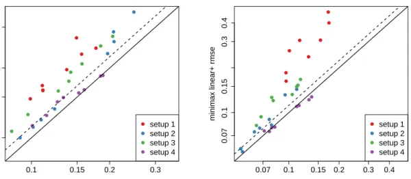
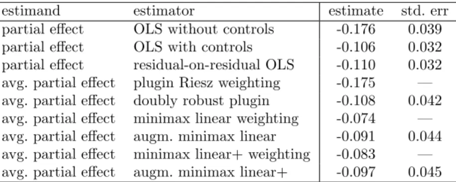
2.1 Performance of AMLE and baselines in simulation. . . 36 2.2 Estimates for the effect of unearned income on earnings using data from Imbens, Rubin,

and Sacerdote (2001). . . 38

List of Figures

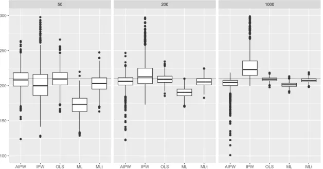
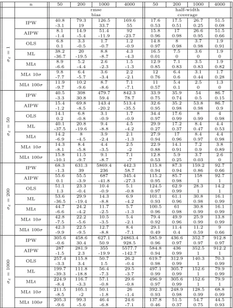
2.1 Comparing augmented minimax linear estimation with linear estimation. . . 35 3.1 Minimax linear estimates in the Kang & Schafer Example . . . 62 3.2 Estimation error in the Kang & Schafer Example . . . 63

(8)

Acknowledgements

I would like to thank Jos´e Zubizarreta for introducing me to Causal Inference as a field and as a community; for his guidance, collaboration, and friendship during my time in graduate school; and for his generosity with his time and ideas. He never gave me his second-best project. Had he not invited me as an inexperienced student to join him in a promising collaboration with Arian Maleki on minimax interpretations of treatment effect estimators, I could not have written this thesis.

I would also like to thank Arian, from whom I learned the basics in my first year as a graduate student and have continued to learn as we’ve worked together since. His advice has been invaluable throughout my time at Columbia, both in the context of our work together and more broadly as I’ve tried to develop an understanding of a diverse and at times bewildering literature.

I am grateful to Stefan Wager, whose intuition and knack for explaining problems simply has been immensely helpful on the projects we’ve worked together on over the last few years and in my attempts to think about new problems. I am also grateful to David Madigan and Michael Sobel for thoughtful comments on my work and on what needs doing in Causal Inference over the years, and to Whitney Newey, from whom I’ve learned much in recent discussions.

I feel lucky to have been a part of the Statistics Department at Columbia and am grateful to everyone there who has taught me, helped me, or worked with me over the last five years, especially Bodhi Sen, Zhiliang Ying, Ming Yuan, Dave Blei, Andrew Gelman, Tian Zheng, Victor de la Pe˜na, Dood Kalicharan, Anthony Cruz, Rohit Patra and Susanna Makela. I also had the good fortune to spend a semester at the Department of Health Care Policy at Harvard Medical School, and I am grateful to Jos´e for inviting me and supporting me during my time there, to Cynthia Hobbs and others there who made that possible, and to students and faculty members I met at Methods Happy Hour and elsewhere at HCP for making me feel welcome.

I would like to thank Michael Black, who taught me how to write and sell a paper while employing me as a computer vision researcher in his group before my time at Columbia, first at Brown and later at MPI T¨ubingen. Also Alex Weiss, Matt Loper, Eric Rachlin, Aggeliki Tsoli, and other folks from Michael’s group who I shared authorship, code, and lunch with during those years.

(9)

Finally, I’d like to thank the friends and roommates I spent much of my time with while I was in New York, Sonia and Tanya Saraiya, Leah Shabshelowitz, Ilana Rothkopf, Tessa Conrad, and Tommy Wu; the Rhode Island and NYC Climbing Communities; my girlfriend Anne Jonas; and my parents Debbe Fate and Larry Hirshberg, my sister Shira Hirshberg, and my brother Dave Stuebe.

(10)

(11)

Chapter One

Introduction

1.1 Observational Studies and Causality

Randomized experiments are the gold standard for comparing treatments and pervasive in many dis-ciplines: medicine, public health, economics, and psychology among them (Hern´an and Robins,2015; Imbens and Rubin, 2015;Rosenbaum, 2002). But often we are interested in comparing treatments we cannot randomize because it is either infeasible or unethical, for example when the comparison is between home and hospital birth (Daysal et al.,2016) or when we are interested in adverse effects of a medication that has already become available (Bernardo et al.,2011). Considering the former, we could compare the rate of infant mortality for babies born at home to that of babies born in hospi-tals, but the result will be difficult to interpret, as association is not causation. Taking a difference of these rates would give us a mixture of the effect of the difference in birth setting and the baseline difference in infant mortality between those who elect home birth and those who elect hospital birth. These groups are systematically different, so it is reasonable to expect a baseline difference, possibly due to age, diet, exposure to toxins, etc. Because of this, the observed difference in infant mortality rates is not necessarily predictive of how the aggregate infant mortality rate would change if home birth became more (or less) popular. If we are able to disentangle the effect of the difference in birth setting from these baseline differences, we have a stronger basis for individual decisionmaking, advocacy, and policy.

However, with rare exceptions, we need to make strong untestable assumptions to disentangle causal effects like this one from baseline differences in observational studies. To discuss these, we need language we can use to define our assumptions. Working with such language has allowed scholars to more precisely define and compare estimands and evaluate estimators (Sobel,2000). In this dissertation, I will use the framework ofpotential outcomes, in which we imagine that for each study participant i and treatment of interest w ∈ W, there is an outcomeY_i(w) that would have happened if, possibly contrary to fact, participantihad received treatmentw(Neyman,1923;Rubin, 1974). The vector all potential outcomes will be writtenY_iW and the index setWcan be arbitrary.

(12)

Categorical indiceswmay represent totally distinct treatments or discrete levels of a treatment dose, continuous indiceswmay represent doses, mixed categorical/continuous indices may represent doses of distinct treatments, etc. We observe onlyWi, indicating which treatment occurred; Yi=Y

(Wi)

i , the outcome under that treatment; and Xi, a vector of covariates describing the participant. I will also assume that our participants are independently drawn from an infinite superpopulation, i.e. the complete data vectors (Xi, Wi, YiW) are independent and identically distributed random variables from some distributionP. In these terms, we define the comparison we want to make, or causal estimand, as a function of this distribution. When the treatmentwis binary, two of the most common are the average treatment effect (ATE),τ:=E[Yi(1)]−E[Y

(0)

i ], and the average treatment effect on the treated (ATT),τT :=E[Yi(1)|Wi= 1]−E[Yi(0)|Wi= 1]. Each of these estimands is a difference in potential outcomes under the two treatments averaged; the ATT is an average over the distribution of all the units in our study whereas the ATT is an average over that of the units that receive treatment.

The assumptions we feel most comfortable making dictate ouridentification strategy, the means by which we convert a causal estimand defined in terms of unobserved potential outcomes, into a statistical estimand, defined in terms of the distribution of the observed data. I will focus on the assumption that no unobserved factor influences both the selection of treatment and the vector of potential outcomes, often calledunconfounded treatment assignment,strong ignorability,selection on observables, orexogenous noise. This assumption justifies estimation of causal effects by adjusting for the observed covariates X. It is rare that any identifying assumptions are satisfied in practice; for that reason once we’ve estimated the statistical estimand, we study how it can deviate from the causal estimand as a function of the degree to which our identifying assumptions are violated. This last step, calledsensitivity analysis, allows in some cases a quantitative defense against arguments that ‘an association does not imply causation.’ This was used convincingly by Cornfield in 1959 when prominent statisticians questioned the causal relationship between cigarettes and lung cancer on that basis (Cornfield et al.,1959).

1.2 Causal Estimands and Identification

In this section, we will consider a simple causal estimand, the ATTτT. First note that Y

(1)

i =Yi when Wi = 1, so the first term in τT is simplyE[Yi | Wi = 1] and can be estimated by a sample mean. The latter term, E[Yi(0) | Wi = 1], is what requires our attention. We make the simplest nontrivial assumption that allows us to estimate it, the unconfoundedness assumption thatE[Yi(0)|

(13)

In order to ensure these expectations are defined, we make a so-called positivity assumption,P{Wi= 1 | Xi} > 0. We call the last expression in (1.1), which is defined in terms of the distribution of the observed data, the statistical estimand. It is a scalar-valued function, henceforth functional, of the conditional mean function m(x, w) = _E[Yi | Xi = x, Wi = w]. In particular, we have E[Yi(0) | Wi = 1] = ψ(m) where ψ(f) = E[f(Xi,0) | Wi = 1] is a linear functional. Many of the simpler causal estimands, including all of those that we will discussed in this dissertation, can be identified as linear functionals of conditional mean functions using essentially this argument. The appropriate unconfoundedness assumption varies slightly depending on the estimand, but the core notion at play is that given covariates, the outcomeY_i(w) that would occur under some fixed treatmentwdoes not depend on the treatmentWi that is actually observed.

1.3 Estimation

Having identified our causal estimand as some kind of function or functional of the observed data, we can now forget about causality until it comes time to do sensitivity analysis. This is slightly cavalier, as some sensitivity analysis methods are available only for estimators of specific forms, but very general and even completely estimator-agnostic approaches are available (seeZhao et al. (2017a) andDing and VanderWeele(2016) respectively). I say this to emphasize that the estimation problems in causal inference need not be the specific domain of the causal inference community — they are ordinary nonparametric or semiparametric estimation problems.

1.3.1 Estimation of Linear Functionals and Riesz Representation

In this dissertation, I focus on semiparametric problems, and in particular on the estimation of continuous linear functionalsψof conditional meansm(x, w).1 _{One of the core objects that we will}

be discussing is the Riesz representerγψ, the unique function that satisfies

Eγψ(Xi, Wi)f(Xi, Wi) =ψ(f) for all square integrable functions f(x, w). (1.2)

1_{The method considered in the first chapter can be applied to linearizations of differentiable functionals around}

(14)

The Riesz representation theorem guarantees that such a function exists and is unique for any continuous functional ψ (see e.g. Peypouquet, 2015, Theorem 1.4.1). The relevant notion of con-tinuity is concon-tinuity in mean square, i.e. ψ(f)≤Ckfk_L

2(P) for all f and some constant C where

kfk_L

2(P)=

p

Ef(Xi, Wi)2. If we knowγψ, we have a good estimator: n−1P n

i=1γψ(Xi, Wi)Yi → E[γψ(Xi, Wi)E[Yi|Xi, Wi]] =ψ(m) atn−1/2 rate by the central limit theorem.

While this sort of Riesz representer is not frequently discussed as a general phenomenon in this context, instances are discussed pervasively. For example, the Riesz representer for the functional

ψ(f) =_E[f(Xi,0)|Wi= 1] that we identified in the context of the ATT is the inverse propensity weighting function2

γψ(w, x) =1{w=0}(1−e(x))

p1e(x) where e(x) =P{Wi= 0|Xi=x}, p1=P{Wi= 1}. This functione(X) is called the propensity score. The ‘overlap’ condition 0< e(x) that we need to identify the ATT implies continuity of the functionalψthat we identify as the ATT. Furthermore, the ‘strong overlap’ condition 0< η≤e(x) that is typically assumed is equivalent to boundedness of the Riesz representerγψ. This boundedness property is almost invariably assumed in the semiparametric estimation literature, and it has in fact been shown byKhan and Tamer (2010) that it is required forn−1/2_{-rate estimation of the ATE and other estimands. We will assume it throughout.}

Estimation of the Riesz representer γψ is straightforward in general, as the defining property (1.2) of the Riesz representer is a set of moment conditions. These moment conditions have been used for some time in the causal inference literature for checking the adequacy of inverse propensity score estimators (see e.g Rubin, 2004) and for estimation of weights that act like γψ (Graham et al., 2012; Hainmueller, 2012; Imai and Ratkovic, 2014; Robins et al., 2007; Zubizarreta, 2012). In that tradition, the approximate satisfaction of the equations (1.2) is called ‘balance,’ and arises from minimax considerations. More recently,Chernozhukov et al.(2016,2018);Newey and Robins (2018) have begun speaking more explicitly about estimating Riesz representers using the moment conditions (1.2), and have done so in fairly general settings. Both influences appear in what follows. In the next chapter, I will discuss a general approach to the estimation of linear functionalsψof conditional mean functionm. The essential approach is to bias-correct simple plugin estimatorψ( ˆm) by subtracting a weighted sum of the regression residualsYi−mˆ(Xi, Wi). The weights we choose solve a sort of minimax problem — minimizing the maximum, over conditional mean functionsmin

2_{It is common to write this without the factor of} _p

1 in the denominator use it in a weighted average

n−1₁ Pn

i=11{Wi=0}(1−e(Xi))/e(Xi)Yi wheren1=

Pn

i=11{Wi=1}, which behaves liken

−1Pn

i=1γψ(Xi, Wi)Yi

(15)

a neighborhood of our estimate ˆm, of the design-conditional mean squared error of the bias-corrected estimator. This minimax criterion demands that our weights act like and ultimately converge to the Riesz representerγψ of our functional, and as a consequence of this behavior we are able to establish semiparametric efficiency under weak regularity conditions for a large class of estimands. This class includes the ATE for a categorical treatment and various generalizations for continuous-valued treatments and individualized treatment assignment policies.

In the chapter following, I focus on the estimation of average treatment effects using minimax linear estimators, a degenerate case of the approach discussed in the first chapter in which we use a trivial estimate ˆm= 0 of the conditional mean. Using a sharper characterization of this estimator’s design-conditional bias than the one offered in the first chapter, I establish semiparametric efficiency for these estimators under similarly weak conditions and characterize the degree to which this first-order asymptotic characterization justifies inference by bounding higher first-order terms.

(16)

Chapter Two

Augmented Minimax Linear Estimation

In this chapter, we address problems in which we observenindependent and identically distributed samples (Zi, Yi)∼P with support inZ ×R, and we want to estimate a continuous linear functional of the form

ψ(m) =_E[h(Zi, m)] at m(z) =EYi

Zi =z. (2.1)

Our main result establishes that we can build efficient estimators for a wide variety of such problems simply by subtracting from a plugin estimatorψ( ˆm) a minimax linear estimate of its errorψ( ˆm)− ψ(m).

The following estimands from the literature on causal inference and missing data are of this type and can be estimated efficiently by our approach.

Example 2.1 (Mean with Outcomes Missing at Random). Suppose we observe covariatesXi and some but not all of the corresponding outcomes Y?

i . Then for an indicator Wi that the outcome

Y_i? was observed, we have observedZi= (Xi, Wi) andYi=WiYi?, and we may estimate the linear functional ψ(m) = E[m(Xi, 1)] at m(x, w) = EYi

Xi=x, Wi=w

. This will be equal to the meanE[Yi?] if, conditional on covariatesXi, each outcomeY

?

i is independent of its nonmissingness

Wi (Rosenbaum and Rubin,1983).

Example 2.2 (Average Partial Effect). LettingZi = (Xi, Wi)∈ X ×R, we estimate the average of the derivative of the response surfacem(x, w) with respect tow, ψ(m) =Edwd {m(Xi, w)}w=Wi

. This estimand—and weighted generalizations of it—present a natural quantification of the average effect of a continuous treatmentWi under exogeneity (Powell, Stock, and Stoker,1989).

Example 2.3 (Average Partial Effect in the Conditionally Linear Model). Considering the estimand discussed in the previous example, we make the additional assumption that the regression function

mis conditionally linear inw,m(x, w) =µ(x) +wτ(x). Then the average partial effect is ψ(m) = E[τ(Xi)] (Robinson,1988).

Example2.4 (Distribution Shift).We estimate the effect of a shift in the distribution of the condition-ing variable Z from one known distribution, P0, to another, P1. ψ(m) = R

(17)

for m(z) =E[Yi|Zi=z]. Under exogeneity assumptions, this estimand can be used to compare policies for assigning personalized treatments, and estimators for it form a key building block in methods for estimation of optimal treatment policies (Athey and Wager,2017).

In this section, we will discuss our estimator in the simple case that our functional of interest

ψ(·) is known, in the sense that given a function f, we are able to evaluate ψ(f). This is the case in Example 2.4. Our problem formulation (2.1) is more general, allowing ψ(·) to depend on the unknown distribution P in a limited way, as E[h(Z,·)] depends on the marginal distribution of Z. We address this sort of dependence later in Section 2.1 by working with sample average approximations toψ(·).

2.0.1 Estimation of Known Linear Functionals

Consider the estimation of ψ(m) whereψ(·) is a known mean-square-continuous linear functional. As discussed in our introductory remarks, the estimator we propose is a plugin estimatorψ( ˆm) with a estimate of its errorψ( ˆm)−ψ(m) =ψ( ˆm−m) subtracted,

ˆ ψ=ψ( ˆm)− 1 n n X i=1 ˆ γi( ˆm(Zi)−Yi). (2.2) Our focus will be on this error estimaten−1Pn

i=1γˆi( ˆm(Zi)−Yi). The existence of a good estimate of this form follows from the Riesz representation theorem, which implies that any continuous linear functionalψ(·) on the square integrable functions from Z to_Rhas a Riesz representerγψ(·), i.e. a function satisfyingE[γψ(Zi)f(Zi)] =ψ(f) for all square-integrable functionsf(see e.g.Peypouquet, 2015, Theorem 1.4.1).

Chernozhukov, Escanciano, Ichimura, and Newey (2016) show that using this function γψ, it is possible to define an oracle estimator of the proposed form. To do this, consider the function

f = ˆm−m, approximate this expectation by a sample average n−1Pn

i=1γi( ˆm(Zi)−m(Zi)) with γi=γψ(Zi), and substitute for the unknown quantity m(Zi) the unbiased estimatorYi:

ψ( ˆm−m) =E[γψ(Z)( ˆm−m)(Z)] ≈ 1 n n X i=1 γi( ˆm(Zi)−m(Zi)) = 1 n n X i=1 γi( ˆm(Zi)−Yi) + 1 n n X i=1 γi(Yi−m(Zi)). (2.3)

As a result, the error of the estimator (2.2) with the oracle weights ˆγi=γψ(Zi) will be roughly equal to a weighted sum of mean-zero noisen−1Pn

i=1γiεiwhereεi=Yi−m(Zi). This behavior is known

(18)

Our goal will be to imitate the behavior of this oracle estimator. One possible approach is to determine the form of the Riesz representerγψ(·) by solving the set of equations that define it,

E[γψ(Z)f(Z)] =ψ(f) for all f satisfying Ef(Z)2<∞, (2.4) then estimate it and plug the resulting weights ˆγi = ˆγψ(Zi) into (2.2). In the context of our first example, the estimation of a mean with outcomes missing, the Riesz representer is the inverse probablility weight γψ(w, x) = w/e(x) where e(x) = P[Wi = 1 | Xi = x], and this approach results in the well-known Augmented Inverse Probability Weighting (AIPW) estimator of Robins and Rotnitzky(1995).

We take another approach. Considering our regression estimator ˆmand the designZ1. . . Znto be fixed1, we simply choose the weights ˆγ∈Rnthat make our correction termn−1Pin=1γˆi( ˆm(Zi)−Yi) a minimax linear estimator of what it is intended to correct for,ψ( ˆm−m). To be precise, we choose the weights that perform best in terms of mean squared error in the worst case over regression functions min a neighborhood ˆm− F of our regression estimator ˆm and over conditional variance functions Var [Yi|Zi =z] bounded byσ2, having chosenF to be an absolutely convex set of func-tions which, given our beliefs about the regression functionmand the properties of our estimator ˆm, should contain the regression error ˆm−m. This specifies the weights ˆγ as the solution to a convex optimization problem, ˆ γ= argmin γ∈Rn I_ψ,2_F(γ) +σ 2 n2kγk 2 , Iψ,F = sup f∈F 1 n n X i=1 γif(Zi)−ψ(f). (2.5) The good properties of minimax linear estimators like this one are well known. Donoho (1994) and related papers (Armstrong and Koles´ar, 2018; Cai and Low, 2003; Donoho and Liu, 1991; Ibragimov and Khas’minskii,1985;Johnstone,2015;Juditsky and Nemirovski,2009) show that when a regression functionm is in a convex setF andYi

Zi ∼N(0, σi2), a minimax linear estimator of a linear functionalψ(m) will come within a factor 1.25 of the minimax risk over all estimators. In addition to strong conceptual support, estimators of the type have been found to perform well in practice across several application areas (Armstrong and Koles´ar, 2018; Imbens and Wager, 2017; Kallus, 2016;Zubizarreta, 2015). Because we ‘augment’ the minimax linear estimator by applying it after regression adjustment in the same way that the AIPW estimator augments the inverse probability weighting estimator, we refer to this approach as the Augmented Minimax Linear (AML) estimator.

1_{If we estimate ˆ}_m_{on an auxilliary sample, this is the case when we condition on both that sample and on}_Z 1. . . Zn.

While it is not necessary to estimate ˆmon an auxilliary sample when estimating linear functionals, we do this in the nonlinear case discussed in a forthcoming commentary (Hirshberg and Wager,2018).

(19)

These weights ˆγ can be interpreted as a penalized least-squares solution to a set of estimating equations suggested by the definition (2.4) of the Riesz representerγψ,

1 n n X i=1 γif(Zi)≈ψ(f) for all f ∈ F (2.6) Note that the restriction off to a strict subsetF of the square-integrable functions is necessary, as there are infinitely many square-integrable functionsfthat agree our sampleZ1. . . Znand they need not even approximately agree in terms ofψ(f). Our choice of this subsetF, a set that characterizes our uncertainty about the regression error function ˆm−m, focuses our estimated weights ˆγon the role they play in our correction term’s derivation (2.3) — the role of ensuring that (2.6) is satisfied for this functionf = ˆm−m. The size of this subsetF, measured e.g. by its Rademacher Complexity, determines the accuracy with which these equations (2.6) can be simultaneously satisfied. So that we do not ‘waste’ accuracy atf = ˆm−mby working with too large a setF, it is helpful to encode the complexity-limiting assumptions that we believe are satisfied by ˆm−min our choice. For example, we may takeF to be a set of smooth functions, functions that are approximately sparse in some basis, functions of bounded variation, etc.

That our weights ˆγi approximately solve these estimating equations (2.6) does not imply that they estimate the Riesz representer γψ(·) well in the mean-square sense. However, to whatever degree the oracle weightsγi=γψ(Zi) also approximately solve (2.6), it will imply that ˆγandγψ(·) are close in the sense that

1

n

X

i=1

[ˆγi−γψ(Zi)]f(Zi)≈0 for allf ∈ F. (2.7) This property will hold if the vector with elements ˆγi−γψ(Zi) is small or if it is approximately orthogonal to the vector with elementsf(Zi) for all functionsf ∈ F, and so long as ˆm−mis in F or a scaled version of it, this will imply that our estimator with weights ˆγiand our oracle estimator with weights γi = γψ(Zi) will be close as well — the difference between them is n−1P

n i=1[ˆγi−

γψ(Zi)][ ˆm(Zi)−m(Zi)−εi].

We state below a simple version of our main result. In essence, if an estimator ˆmconverges tom

in mean square and our regression error ˆm−mis in a uniformly bounded Donsker classF or more generally satisfies ( ˆm−m)/Op(1)∈ F, then our approach can be used to define an asymptotically efficient estimator of a known continuous linear functionalψ(m) atm(z) =E[Yi|Zi=z].

2.0.2 Definitions

As a measure of the scale of a functionf relative to an absolutely convex setF, we define thegauge2

(20)

{f :n−1Pn

i=1 f(Zi)

2_≤₁_}_{, so that the gauges} _k·k

L2(P) and k·kL2(Pn) have their typical meanings as the root mean squared error and empirical root mean squared error. We will writeMto denote the closure of a subspace M of the square-integrable functions and will also also write spanF to denote the closure of spanF. We say a class F is pointwise separable if it has a countable subset

F0 such that for every functionf ∈ F, there is a sequence fm∈ F0 converging to g pointwise and

ink·k_L

2(P) (see, e.g.,van der Vaart and Wellner, 1996, section 2.3.3).

2.0.3 Setting

We observe (Y1, Z1). . .(Yn, Zn) iid

∼ P withYi ∈R, Zi∈ Z for a complete separable metric spaceZ. We assume thatm(z) =_EP[Yi |Zi =z] is in a subspaceMof the square integrable functions and thatv(z) = Var [Yi|Zi=z] is bounded. And we letF be absolutely convex set of square integrable functionsF that believed to contain, at least up to scale, the regression error ˆm−m.

Our estimand isψ(m) for a known and continuous linear functionalψ(·) on a subspaceM∪spanF

of the square integrable functions. The Riesz representation theorem guarantees the existence and uniqueness of a functionγψ ∈spanF satisfying the set of equations {EPγψ(Z)f(Z) =ψ(f) :f ∈ spanF }.3 _{We call this function the Riesz representer of}_ψ_{on the}_{tangent space} _span_F _{and observe}

that when spanF is the space of square integrable functions, this agrees with our prior definition (2.4).

We will assume thatψ(·) satisfies the following continuity property, which ensures that our Riesz representerγψ is bounded.4

kψk_L?

1(P)<∞forkψkL?1(P):= _f_∈sup_span_F

kfk_L

1 (P)≤1

ψ(f). (2.8)

Theorem 2.1. In the setting above, consider the estimator

ˆ ψAM L=ψ( ˆm)− 1 n n X i=1 ˆ γi( ˆm(Zi)−Yi), ˆ γ= argmin γ∈Rn I_ψ,2_F˜_n(γ) + σ2 n2kγk 2 , Iψ,F = sup f∈F 1 n n X i=1 γif(Zi)−ψ(f). (2.9)

2_{We write the gauge}_k·k

F because for the setsF we will be working with, the gauge is a norm. While in general,

the gauge of an absolutely convex set is a pseudonorm, we will be working with sets for which point evaluation is gauge-continuous, i.e. f(x)≤c(x)kfk_F forc(x)<∞, and which therefore satisfykfk_F= 0 =⇒ f(x) = 0 for allx.

3_{In this statement we implicitly work with the unique extension of the continuous functional} _ψ(_·_{) defined on}

spanF to a functional defined on its closure spanF(Lang,1993, Theorem IV.3.1).

4_{Boundedness of the Riesz representer}_γ

ψfollows from the Hahn-Banach extension theorem (Lang,1993, Theorem

IV.1.1), which guarantees that the equivalent linear functionalsf →ψ(f) and f →_E

γψ(Z)f(Z)

defined on the tangent space have an extension to the spaceL1(P) of all integrable functions which satisfies the samek·kL?

1(P)bound

and therefore satisfieskγψk∞= supf∈L1(P)E

γψ(Z)f(Z)

(21)

for F˜n = F ∩ρnL2(Pn), ρn ∈ R+ ∪ {∞} satisfying n1/2ρn → ∞, and any finite σ > 0. If F is a pointwise separable uniformly bounded Donsker class, then the weights converge to the Riesz representer ofψon the tangent space spanF in the sense

1 n n X i=1 (ˆγi−γψ(Zi))2→P 0. (2.10)

If, in addition, mˆ has the tightness and consistency properties a. kmˆ −mk_F∈ OP(1) andkmˆ −mkL2(Pn)∈ OP(ρn)if ρn →0,

b. kmˆ −mk_F∈oP(1)otherwise,

then our estimatorψˆAM L has the asymptotic linear characterization ˆ ψAM L−ψ(m) = 1 n n X i=1 ι(Yi, Zi) +oP(n−1/2) where ι(y, z) =γψ(z)(y−m(z)) (2.11)

and therefore √n( ˆψAM L−ψ(m))/V1/2 ⇒ N(0,1) with V = Eι(Y, Z)2. When this happens, ˆ

ψAM L is regular if M ⊆spanF and is semiparametrically efficient iff it is regular andv(·)γψ(·)∈

M.

This theorem is a straightforward consequence of a more general asymptotic result, Theorem2.4, discussed in SectionA.1. It is proven in AppendixA.1. We end this section with a few remarks. Remark 2.1. Our assumptions boil down to continuity of the functional ψ(·) and the tightness and consistency properties kmˆ −mk_F ∈ OP(1) and kmˆ −mkL2(Pn) ∈ OP(ρn) that we require of our estimator. While we can do nothing about the continuity of the functional ψ(·), there is a general recipe for ensuring these tightness and consistency properties. If we can choose F to be an absolutely convex Donsker class such that kmk_F < ∞, then the estimator ˆm minimizing the penalized empirical riskn−1Pn

i=1(Yi−m(Zi))2+λkmk ν

Ffor appropriately chosenλ, νwill typically

have these properties withρn =n−1/4 (see e.g. Lecu´e et al.(2018, Theorem 3.2) and van de Geer (2000, Theorem 10.2)).

Remark 2.2. Our estimator does not require knowledge of the form of the Riesz representerγψ(·). This spares us the trouble of determining it for each estimand we consider. And while our efficiency condition v(·)γψ(·) ∈ M is phrased in terms of γψ, we can often think in terms of the sufficient condition{v(·)f(·) :f ∈spanF } ⊆ M.

Remark 2.3. We note two particular ways to define our weights in this theorem. A simple approach is to just takeρn =∞, which results in weights which control our error uniformly over functions

(22)

in a fixed class F. This takes advantage of the decay of the regression error ˆm−m as measured by the gauge k·k_F, a very strong type of convergence, but not its decay in any weaker norm like

k·k_L

2(Pn). In this case, our theorem applies if ˆm is k·kF-consistent for m. However, we can also exploit a known rate of convergenceρnfor ˆm−mink·kL2(Pn)to work uniformly over a smaller class

˜

Fn=F ∩ρnL2(Pn) appropriate to our sample size; in this case, it is sufficient to have tightness of ˆ

m−min k·k_F rather than consistency.

Remark 2.4. This theorem is valid in the general case that ψ(m) =_E[h(Zi, m)] if we substitute ˜

ψ(·) =n−1Pn

i=1h(Zi,·) forψ(·) where it appears in (2.9), change the influence function toι(y, z) =

h(z, m)−ψ(m) +γψ(y−m(z)), and make the additional assumptions that (i){h(z, f) :f ∈ F }is a pointwise separable uniformly bounded Donsker class and that (ii)h(Z, f) is uniformly continuous at zero in the sense that sup_f_{∈F ∩}_rL₂₍_P₎Var [h(Z, f)]1/2→0 asr→0. This is proven in AppendixA.1. Remark 2.5. Our estimator ˆψAM Lis defined in terms of an estimator ˆmof our regression function and the classFof possible regression errors ˆm−mthat we correct for. The choices we make for ˆmand

F correspond to assumptions about the regression functionm. In addition to complexity-limiting assumptions like smoothness, we may in some cases choose to make parametric or semiparametric assumptions about the form of the model. Such an assumption distinguishes Examples2.2and2.3, which consider the Average Partial Effect for arbitrary functions m(w, x) and for functions of the formm(w, x) =µ(x) +wτ(x) respectively.

In the latter case, which we discuss in detail in Section2.2, it is natural to use an estimator ˆmof this form and to takeF to be a class of functions having this form. As a result, the tangent space spanF is smaller than the space of all square integrable functions, and the Riesz representerγF for

ψ(·) will be the orthogonal projection of the Riesz representerγL2 forψ(·) on the tangent space of all

square-integrable functions onto spanF. An important consequence is that the optimal asymptotic variance in Example2.3is strictly lower than that in Example2.2so long as our stated conditions for efficiency are satisfied.5 This reflects the ease of estimating the APE in the Conditionally Linear Model relative to the general case.

We pay for this reduction in asymptotic variance with a corresponding reduction in robust-ness. When these parametric or semiparametric assumptions are violated and ˆm−m /∈ spanF, the theorem above says nothing about the performance of our estimator. Characterization of the behavior of our estimator in settings in which these assumptions tend to be violated in practice, as in Example2.2, is important but beyond the scope of this paper.

5 _{The the difference in asymptotic variance between estimators using weights converging to} _γ

L2

(Exam-ple 2.2) and weights converging to γF (Example 2.3) is Ev(Z)[γL22(Z)−γ

2

F(Z)] = Ev(Z)[γL2(Z)−γF(Z)]

(23)

Remark 2.6. Although we assume no regularity conditions on the Riesz representer γψ(·) beyond boundedness, our weights ˆγi still estimate it consistently. This is a universal consistency result, in line with well known results aboutk-nearest neighbors regression and related estimators (Lugosi and Zeger,1995;Stone,1977). Heuristically, the reason for this phenomenon is that the Riesz representer

γψ is the unique6weighting function that sets a population-analogue ofIψ,F to 0; because ˆγ comes

close to doing the same, it must also approximate γψ. This universal consistency property is not what controls the bias of our estimator ˆψ (in fact the rate of convergence of ˆγi to γψ(Xi) is in general too slow for standard arguments for plugin estimators to apply); however, it plays a key role in understanding why we get efficiency under heteroskedasticity even though we choose our weights by solving an optimization problem (2.5) that is not calibrated to the conditional variance structure ofYi.

To understand this phenomenon, observe that under the conditions of Theorem2.1, the condi-tional bias termn−1Pn

i=1ˆγi( ˆm(Zi)−m(Zi)) in our error isoP(n−1/2). It is therefore unnecessary to make an optimal bias-variance tradeoff by this sort of calibration to get efficiency under het-eroskedasticity and hethet-eroskedasticity-robust confidence intervals; the asymptotic behavior of our estimator is determined by the asymptotic behavior of our noise termn−1Pn

i=1ˆγiεi and therefore by the limiting weightsγψ(Zi).

For the same reason, it is not necessary to know the error scalekmˆ−mk_F to form asymptotically valid confidence intervals. We stress that this is an asymptotic statement; in finite samples, there are strong impossibility results for uniform inference that is adaptive to the scale of an unknown sig-nal(Armstrong and Koles´ar, 2018). Furthermore, tuning approaches that estimate and incorporate individual variancesσi into the minimax weighting problem (2.5) like those discussed inArmstrong and Koles´ar(2018) may offer some finite-sample improvement.

2.0.4 Comparison with Double-Robust Estimation

Perhaps the most popular existing paradigm for building semiparametrically efficient estimators in this setting is via constructions that first compute stand-alone estimates ˆm(·) and ˆγψ(·) for the regression function and the Riesz representer, and then plug them into (Chernozhukov et al.,2016; 2Ev(Z)γF(Z)[γL2(Z)−γF(Z)]. The first term in this decomposition is positive and the second term is zero if

v(·)γF(·)∈spanF, as in this case thereforeEγL2(Z)[v(Z)γF(Z)] =ψ(v(Z)γF(Z)) =EγF[v(Z)γF]. This condition

is satisfied under our efficiency conditions.

6_{This uniqueness is violated when the tangent space span}_F _that _ψ_{acts on is not dense in the space of square}

integrable functions. However, the dual characterization Lemma2.5 shows that our weights must converge to a function in the closure of this tangent space, and it follows that they converge to the unique Riesz representerγψ on

(24)

Newey,1994;Robins and Rotnitzky,1995) ˆ ψDR=γ( ˆm)− 1 n n X i=1 ˆ γψ(Zi) ( ˆm(Zi)−Yi) (2.12) or an asymptotically equivalent expression (see e.g.van der Laan and Rubin,2006). This estimator has a long history in the context of many specific estimands, e.g. the aforementioned AIPW estimator for the estimation of a mean with outcomes missing at random (Cassel, S¨arndal, and Wretman,1976; Robins, Rotnitzky, and Zhao, 1994). In recent work, Chernozhukov, Newey, and Robins (2018) describe a general approach of this type, making use of a novel estimator for the Riesz representer of a functionalγψ in high dimensions motivated by the Dantzig selector ofCand`es and Tao(2007). In considerable generality, this estimator ˆψDR is efficient when we use sample splitting7 to construct ˆmand ˆγψ and these estimators satisfy

1 n n X i=1 [ˆγψ(Zi)−γψ(Zi)][ ˆm(Zi)−m(Zi)]∈oP(n−1/2) (2.13) (Chernozhukov et al., 2017; Zheng and van der Laan, 2011). Taking the Cauchy-Schwartz bound on this bilinear form results in the well known sufficient condition on the product of the errors,

kγˆψ−γψkL2(Pn)kmˆ −mkL2(Pn)∈oP(n

−1/2_{). This phenomenon, that we can trade off accuracy in}

how well the two nuisance functionsmandγψ are estimated, is calleddouble-robustness.

While the estimator ˆψAM L defined in (2.9) shares the form of ˆψDR, it is in no reasonable sense doubly robust. This is by design. The weights ˆγ used in ˆψAM L are optimized for the task of correcting the error of the plugin estimator ψ( ˆm) when our assumptions on the regression error function ˆm−m are correct. When this is the case and the classF characterizing our uncertainty about this function is sufficiently small (e.g. Donsker), this allows us to be completely robust to the difficulty of estimating the Riesz representer γψ. Our estimator will be efficient essentially because the error ˆγ−γψ will be sufficiently orthogonal to all functionsf ∈ F that (2.13) will be satisfied uniformly over the class of possible regression error functions ˆm−m∈ F. As the existence of an estimator ˆm whose error ˆm−m is tight in the gauge of some Donsker class F is essentially equivalent to the existence of anoP(n−1/4)-consistent regression estimator ofm, one way to interpret this is that our use of minimax linear weights ˆγi rather than plug-in estimates ofγψ(Zi) has let us completely eliminate the regularity requirements on the Riesz representer γψ while requiring the same level of regularity on the regression functionm(·).

On the other hand, we sacrifice robustness to the difficulty of estimating the regression function

m. In terms of the regularity assumptions necessary for asymptotic efficiency, ˆψDR is preferable to

7_{In particular, this result holds if we use the cross-fitting construction of} _Schick _{(1986), where separate data}

folds are used to estimate the nuisance components ˆm(·) and ˆγψ(·) and to compute the expression (2.12) given those

(25)

ˆ

ψAM L whenever estimates of γψ with faster than OP(n−1/4) convergence are available (and vice-versa). Furthermore, for some specific choices of estimators ˆγψ(·) and ˆm(·), it has been shown that the errors in estimating the nuisance parameters are sufficiently orthogonal that the rate-product bound can be relaxed (Newey and Robins,2018). Thus, our aim is by no means to suggest that the AMLE dominates existing doubly-robust methods, but rather only to show that the approach can achieve efficiency under surprisingly general conditions.

In addition, we typically sacrifice robustness to any semiparametric or parametric assumptions we make on the form our regression functionm. For example, when estimating a mean with outcomes missing at random in a high-dimensional linear modelm(w, z) =wxT_β_{, it is natural to control error} over a set F of similar linear models. In this case, the Riesz representer for ψ(·) on the tangent space spanF will be not the inverse propensity weightw/e(x) but its best linear approximation. This can result in greater efficiency of estimation than using the true or estimated inverse propensity weights but it does not correct for misspecification of the linear model as the use of inverse propensity weights would. This phenomenon is not unique to our approach, as some other methods can estimate something like a Riesz representer on a tangent space of their choosing. See e.g. Remark 2.5 of Chernozhukov et al.(2017) or Section 3 ofRobins et al. (2007).

Thus, while our estimator (2.9) can potentially be seen as an instance of (2.12) because our weights ˆγi do converge to γψ(Zi), the way the two estimators work is very different. Convergence of our weights to the Riesz representer is slow and plays only a second-order role in our analysis. The reason our weights succeed in debiasing ψ( ˆm) is the form of the optimization problem (2.5), not our universal consistency result. Thus, we often find it more helpful to think of our method in the context of minimax linear estimation rather than that of doubly robust methods.

However, these two approaches are not really discrete alternatives. The following section’s The-orem 2.2shows that our weights ˆγwill, if our tuning parameter σin (2.9) is allowed to grow with sample size at the correct rate, typically give a rate-optimal estimate of the Riesz representer ˆγψ. Thus, by varying this parameter σ in our estimator (2.9), we trace out a family of estimators in-cluding the AMLE and a doubly-robust estimator using a very reasonable estimate of ˆγψ. This is discussed briefly in Appendix A.1. In this paper, we will focus on the AMLE case, deferring the exploration of this continuum and strategies for choosing this tuning parameterσto later work.

2.0.5 Related Work

As discussed above, our approach is primarily motivated as a refinement of minimax linear estimators as developed and studied by a large community over the past decades (Armstrong and Koles´ar,2018;

(26)

Cai and Low,2003;Donoho,1994;Donoho and Liu,1991;Ibragimov and Khas’minskii,1985;Imbens and Wager,2017;Johnstone,2015;Juditsky and Nemirovski,2009;Kallus,2016;Zubizarreta,2015); meanwhile, our main efficiency result is most closely comparable to results from the literature on semiparametrically efficient inference, including results on doubly robust methods (Belloni et al., 2017; Bickel et al., 1998; Chen et al., 2008; Chernozhukov et al., 2017, 2018; Farrell, 2015; Hahn, 1998;Hirano et al.,2003;Mukherjee et al.,2017;Newey,1994;Newey and Robins,2018;Scharfstein et al.,1999;Robins and Rotnitzky,1995;Robins et al.,2017;van der Laan and Robins,2003;van der Laan and Rose,2011;van der Vaart,1991).

We are aware of two estimators that can be understood as special cases of our augmented minimax linear estimator (2.2). In the case of parameter estimation in high-dimensional linear models, Javanmard and Montanari (2014) propose a type of debiased lasso that combines a lasso regression adjustment with weights that debias the L1-ball (i.e., a convex class known to capture

the error of the lasso); meanwhile, Athey, Imbens, and Wager (2016) develop a related idea for average treatment effect estimation with high-dimensional confounding. The contribution of our paper relative to this line of work lies in the generality of our results, and also in characterizing the asymptotic variance of the estimator under heteroskedasticity and proving efficiency in the fixed-dimensional nonparametric setting. Given heteroskedasticity, Athey, Imbens, and Wager (2016) and Javanmard and Montanari (2014) only prove√n-consistency but do not characterize the the asymptotic variance directly in terms of the distribution of the data; rather, they have an expression for the variance that depends explicitly on the solution to an optimization problem analogous to (2.5).

In the special case of mean estimation with data missing at random, the optimization problem (2.5) takes on a particularly intuitive form, and

IF = sup f∈F 1 n n X i=1 (1−Wiˆγi)f(Xi,1) (2.14) measures how well the ˆγ-weighted average off over the observed samples matches its average over everyone. In other words, the minimax linear weights enforce “balance”, which has been emphasized as fundamental to this problem by several authors including Rosenbaum and Rubin (1983) and Hirano, Imbens, and Ridder(2003). More recently, there has been considerable interest in practical methodologies that emphasize balance when paired with AIPW methodology (Athey et al., 2016; Chan et al., 2015; Graham et al., 2012, 2016; Hainmueller, 2012; Hirano et al., 2001, 2003; Imai and Ratkovic,2014;Kallus,2016;Wang and Zubizarreta, 2017; Zhao,2016;Zubizarreta,2015). In addition to generalizing beyond the missing-at-random problem, our Theorem2.4also provides the

(27)

sharpest results we are aware of for balancing-type estimators in this specific problem.

2.1 Estimating Linear Functionals

In this section, we will address the problem of estimating continuous linear functionals of the form

ψ(m) =E[h(Z, m)] atm=E[Yi|Zi=z]. We will be working with a generalization of the estimator described in the previous section that substitutes sample averages ofh(Zi,·) for the possibly unknown functionalψ(·), ˆ ψAM L= 1 n n X i=1 h(Zi,mˆ)− 1 n n X i=1 ˆ γi( ˆm(Zi)−Yi), ˆ γ= argmin γ∈Rn I_h,2 _˜ F(γ) + σ2 n2kγk 2 , Ih,F= sup f∈F 1 n n X i=1 [γif(Zi)−h(Zi, f)]. (2.15)

Note that in the case thatψ(·) is known,h(Zi,·) =ψ(·) for allZi, and this reduces to our estimator from Theorem2.1when we take ˜F =F ∩ρnL2(Pn). Here we allow ˜Fto be an arbitrary set defined in terms ofZ1. . . Zn and we will characterize our estimator primarily in terms of a pair of nonrandom ‘bounds’FL andF satisfyingFL ⊆F ⊆ F˜ with high probability.

To better understand the behavior of our estimator, we decompose its error into a bias-like term and a noise-like term. We will consider estimation of a sample-average version of our estimand,

˜

ψ(m) :=n−1Pn

i=1h(Zi, m), as the behavior of the latter term in the error decomposition ˆψAM L−

ψ(m) = ( ˆψ−ψ˜(m)) + ( ˜ψ(m)−ψ(m)) is entirely out of our hands. We write ˆ ψAM L−ψ˜(m) = 1 n n X i=1 (h(Zi,mˆ)−h(Zi, m))−γˆi( ˆm(Zi)−Yi) = 1 n n X i=1 h(Zi,mˆ −m)−γˆi( ˆm−m)(Zi) | {z } bias + ˆγi(Yi−m(Zi)) | {z } noise . (2.16)

We will establish finite sample bounds on the bias term and the difference between the noise term and the noise term of the oracle estimator with weights γψ(Zi). If both of these quanti-ties are op(n−1/2_{), our estimator will be asymptotically linear with influence function} _ι₍_{y, z}_{) =} h(z, m)−ψ(m) +γψ(z)(y−m(z)), which implies asymptotic efficiency under a few conditions stated in Proposition2.3.

We establish these bounds in essentially three steps. 1. Establish a bound onn−1Pn

i=1(ˆγi−γ?i)2 forγi?=γψ(Zi).

2. Our bias term can be bounded by kmˆ −mk_F˜I_h,_F˜(ˆγ). Observe that as a consequence of the

definition of our weights ˆγin (2.15), they satisfy

I_h,_F˜(ˆγ)2≤I_h,_F˜(γ?)2+ σ2 n2 n X i=1 γ_i?2−γˆ_i2. (2.17)

(28)

Empirical process techniques can be used to characterize the first term in this bound, as the weights γ? _{have the property that} _I

h,F(γ?) is the supremum of the empirical process

n−1Pn

i=1δXi indexed by the class of mean-zero functionsH={z→h(z, f)−γψ(z)f(z) :f ∈

F }, while the second term can be bounded using the previous step and some simple arithmetic. This bound, in combination with a bound onkmˆ −mk_F˜, will imply a bound on our bias term.

3. Bound the difference between our noise term and that of the oracle estimator,n−1Pn

i=1(ˆγi− γ?

i)(Yi−m(Zi)), using our the first step.

The first step represents the core technical contribution of our paper. Following a few definitions, we will state and prove these bounds.

2.1.1 Definitions

As it will be useful to discuss the behavior ofh(Zi, f) forf ∈ F −γψ, ifγψ ∈/ spanF we will we will work implicitly with the extension of thez-indexed family of linear functionalsh(z,·) to the space spanned by this set that satisfiesh(z, γψ) =γψ(z)2 for allz. Note that when working on this larger space,γψ is still a Riesz representer, asψ(f) =E[h(Zi, f)] =E[γψ(Zi)f(Zi)] for allf in it. It will often be convenient to work on a slight enlargement of this set, F −[0,1]γψ, which is star-shaped around zero.

To characterize the size of a set G, we will use its Rademacher complexity, defined Rn(G) := Esupg∈G|n−1

Pn

i=1ig(Zi)| where i =±1 each with probability 1/2 independently and indepen-dently of the sequence Z1. . . Zn. A useful type of fixed point of the Rademacher complexity of a parameterized family of classes G(r) will be written R?

n(c,G(r)) := inf{r > 0 : Rn(G(r))≤ cr2}. In this context, we will take G(r) = F ∩rL2(P) or a related class, and we call Rn(G(r)) a local Rademacher Complexity (see, e.g., Bartlett et al., 2005; Koltchinskii, 2006). We will also use its maximal supremum normMG := supg∈Gkgk∞.

We will be interested in the Rademacher complexity and local Rademacher complexities of the classesF(r) =F ∩rL2(P),H(r) ={h(z, f)−γψ(z)f(z) :f ∈ F(r)},F?₍_r_{) = (}_{F −}_[0_,_1]_γ_ψ)_∩_rL2₍_P_),

H?₍_r_{) =} _{_h₍_{z, f}₎₋_γ

ψ(z)f(z) : f ∈ F?(r)}, and as a shorthand will write H = H(∞),F? =

F?₍_∞₎_,_H? ₌ _H?₍_∞_{) for the non-localized versions. Specifically, the primary factors determining} our bound will be a measure rQ of the local complexity of F?, measures u(H) and rC of the complexity and local complexity of the classesHandH?_{, and a measure}_κ_{of the degree of}_k·k

FL -size necessary to approximateγψwell. We define these measures, which are similar to those inLecu´e and Mendelson(2017), below.

(29)

rQ(ηQ) = p 24(1 +ηQ) 1−ηQ R?n ₁ 2MF? ,F?₍_·₎ ; rC(ηC, δ) = infr >0 :u(H?(r), δ)≤ηCr2 where u(H, δ)>sup h∈H n−1 n X i=1 h(Zi) with probability 1−δ;8 κ2(σ, δ) = inf ˜ γ ( kγ˜−γψk2_L₂₍_P₎+ δσ2_k_γ_˜_k2 FL 2n ) ; (2.18)

It may be helpful to have a sense of the behavior of these quantities before we state our main result. If ˜F has an upper bound F that is a Donsker class, typically the local complexity fixed pointsrQ(ηQ) andrC(ηC, δ) will beo(n−1/4) and u(Hn, δ) will beO(n−1/2) — typically the latter will beo(n−1/2_{) when we exploit the consistency of the regression ˆ}_m_{by choosing ˜}_F

n satisfying with high probability sup_f_∈_F˜_nkfkL2(P)→0.

9 _{And for fixed} _{σ >}_{0, we will have} _κ₍_{σ, δ}₎_→_{0 essentially}

without assumptions. Roughly speaking, these properties will be sufficient to establish asymptotic results analogous to Theorem2.1.

2.1.2 Main Results

Theorem 2.2. Suppose that we observe iid (Y1, Z1). . .(Yn, Zn) with Yi ∈ R, Zi in an arbitrary set Z, and v(z) = Var [Yi|Zi=z] bounded. Let {h(z,·) :z∈ Z} be a family of linear functionals and the linear functional ψ(·) =E[h(Zi,·)]be continuous. Consider the estimatorψˆAM L defined in (2.15) in terms of σ >0 and an absolutely convex set F˜ defined in terms ofZ1. . . Zn. Let there exist nonrandom sets FL andF satisfying FL ⊆F ⊆ F˜ with probability 1−δ_F˜ with F pointwise

separable, absolutely convex, and either reflexive or totally bounded ink·k_∞. If{h(z, f) :f ∈ F }is pointwise separable andh(Z1,·). . . h(Zn,·)are continuous on the normed vector space(spanF,k·kF)

and on(spanF,k·k_∞)as well if the former space is not reflexive, then on an event of probability at least1−exp{−c1(ηQ)nrQ(ηQ)2/MF2?} −5δ−2δ_F˜,

1. The weightsγˆ defined in (2.15)satisfy n−1Pn

i=1(ˆγi−γˆψ(Zi))2≤a∧b where

8_{We may use the bound}_u(_H_{, δ) = 2δ}−1_R

n(H), which arises from Markov’s inequality and symmetrization (see

e.g.van der Vaart and Wellner,1996, Lemma 2.3.1). Bounds based on Talagrand-type concentration inequalities (see e.g.Bartlett et al.,2005, Theorem 2.1) offer much weaker dependence onδwhen suph∈HkhkL2(P) is comparable to

Rn(H), which will typically be the case.

9_{This is tantamount to saying that the deviation of an empirical process from its mean is}_o

p(n−1/2) when the

class indexing it decays to zero ink·k_L

2(P), a phenomenon typically referred to as the asymptotic equicontinuity of

(30)

a=αu(H?_{, δ}_{) + ¯}_R_; b= 2α2r2∨2 ¯ R+σ2_/n ηQ−2α−1ηC ∨ 44M 2 F?α2log(δ−1) n ; r=rQ(ηQ)∨rC(ηC)∨ση−_Q1/2n−1/2; α= 1∨h2ηCσ−2nr2+σ−1n1/2R¯1/2 i ¯ R= 2δ−_˜1 F κ2+ 2σ−1κσ(H?₍_κ₎₎ + 4δ−_˜1/2 F n −1/2_σ₍_H?₍_κ₎₎_{, κ}₌_κ₍_{σ, δ} ˜ F). (2.19)

2. The uniform version of our bias term satisfies the bound

I_h,_F˜≤u(H, δ) + 21/2kγψk

1/2

L2(Pn)σn

−1/2₍_a_∧_b₎1/4_. _(2.20)

3. The difference between our noise term and that of the oracle estimator satisfies

n−1 n X i=1 (ˆγi−γψ)(Y −m(Zi)) ≤δ−1/2kvk_∞n−1/2(a∧b)1/2. (2.21) Here ηQ∈(0, .47)andηC>0 are arbitrary and the functionc2 is defined in Lemma 2.7.

These bounds yield straightforward conditions under which our estimator is asymptotically linear, i.e. ˆ ψAM L−ψ˜(m) =n−1 n X i=1 ˜ι(Yi, Zi) +oP(n−1/2), ˜ι(y, z) =γψ(z)(y−m(z)); therefore ˆ ψAM L−ψ(m) =n−1 n X i=1 ι(Yi, Zi) +oP(n−1/2), ι(y, z) =h(z, m)−ψ(m) + ˜ι(y, z). (2.22)

Typically, such estimators are asymptotically efficient. The following proposition, proven in Ap-pendixA.1.4, generalizes the conditions for efficiency stated in Theorem2.1

Proposition 2.3. Suppose we observe an iid sample (Zi, Yi)i≤n from P where Yi ∈ R and Zi ∈

Z, a complete separable metric space, and that the set of possible regression functions m(z) = E[Yi|Zi=z] is a linear space M. An estimator for a continuous linear functional of the form

ψ(m) = E[h(Zi, m)] at m(z) = E[Yi|Zi=z] is regular if (2.22) holds where γψ is the Riesz representer for the functionalψ(·)on a space containing the closure ofM. It is semiparametrically efficient if, in addition, the functionz→γψ(z) Var [Yi|Zi =z]is in the closure ofM.

Now consider the expansion of our estimator around this characterization.

ˆ ψAM L−ψ˜(m)− 1 n n X i=1 ˜ ι(Yi, Zi) ≤ 1 n n X i=1 [h(Zi,mˆ −m)−ˆγi( ˆm−m)(Zi)] + 1 n n X i=1 (ˆγi−γψ)(Y −m(Zi)) ≤ kmˆ −mk_F˜I_h,_F˜(ˆγ) + 1 n n X i=1 (ˆγi−γψ)(Yi−m(Zi)). (2.23)

(31)

This difference will be negligible if both the product ofkmˆ −mk_F˜ and our bound (2.20) and our

bound (2.21) areoP(n−1/2). An inspection of these bounds, which we carry out in Appendix A.1, shows that this happens under conditions generalizing those of Theorem2.1. This yields the following asymptotic result.

Theorem 2.4. Let (Zi,n, Yi,n)i≤n be an iid sample from Pn withYi,n∈R,Zi,n in an arbitrary set

Zn, andvn(z) = Var [Yi,n|Zi,n=z]bounded uniformly inn, and definemn(z) =E[Yi,n|Zi,n=z]. In terms of a family of linear functionals{hn(z,·) :z∈ Zn}, define the continuous linear functional

ψn(·) = E[h(Zi,n,·)]. Choose F˜n to be an absolutely convex set, defined in terms of Z1. . . Zn, of square integrable functions on Zn. In terms of that set, an estimator mˆ for mn, and tuning parametersσn=O(1), define the estimator

ˆ ψ= 1 n n X i=1 hn(Zi,n,mˆ)− 1 n n X i=1 ˆ γi( ˆm(Zi,n)−Yi,n), ˆ γ= argmin γ∈Rn I_h2 n,F˜n(γ) + σ2 n n2kγk 2 , Ih,F = sup f∈F 1 n n X i=1 [γif(Zi,n)−h(Zi,n, f)]. (2.24)

Let there exist nonrandom setsFL,nandFn such thatPn{FL,n ⊆F˜n⊆ Fn} →1withFn point-wise separable and either reflexive or totally bounded ink·k_∞; letγψn be the Riesz representer ofψn on the tangent space spanFn; and define Hn(r),Fn?(r),H?n(r)as is Section 2.1.1 in terms of Fn,

hn, andγψn. Then if

i. for each Zi,n, the functional h(Zi,n,·) is continuous on (spanFn,k·k_F_n) and if this space is not reflexive, on(spanFn,k·k∞)as well.

ii. our functional ψn(·) satisfies the condition sup{|ψn(f)| : f ∈ Fn,kfkL1(Pn) ≤ 1} = O(1),

which is equivalent to uniform boundedness of its Riesz representer;

iii. its Riesz representer is approximable in the sense that there exist functions˜γnsatisfyingk˜γn−

γψnkL2(Pn)→0 andk˜γnkFL,n=o(n

1/2_);

iv. Fn is uniformly bounded in the sense that MFn=O(1);

v. R?_n(1,F? n(·)), R ? n(1,H ? n(·)) =o(n− 1/4_); vi. kmˆ −mk_F˜_n=OPn(1),Rn(Hn) =O_Pn(n−1/2),kmˆ −mk_˜ FnRn(Hn) =oPn(n −1/2_);

(32)

our weights ˆγconverge to the Riesz representer and our estimator ψˆis asymptotically linear, i.e. n−1 n X i=1 (ˆγi−γˆψn(Zi,n))→Pn0; (2.25) ˆ ψ−ψn(mn) =n−1 n X i=1

ιn(Yi,n, Zi,n) +oPn(n−1/2) with (2.26)

ιn(y, z) =hn(z, mn)−ψn(mn) +γψn(z)(y−m(z))

Here our assumptions (i,ii,iv) are triangular-array equivalents of assumptions stated in Theo-rem2.1; (v,vi) generalize the Donskerity assumption and assumptions on the tightness and consis-tency of ˆmin Theorem2.1for the estimation of a non-known functional and to the triangular-array setting; and (iii) is a new assumption that is essentially vacuous in the non-triangular asymptotic setting (Pn ₌_P_{). This is the case for (iii) because any fixed function in span}_F _including_γ

ψ can be approximated by a sequence ˜γn with kγ˜nk_F → ∞. We need to include this condition in the triangular-array asymptotics because γψn is not a fixed function. It may, for example, be be a function of increasing dimension.

When our estimator has the asymptotic characterization (2.26),√n( ˆψ−ψn(mn)) is asymptoti-cally normal with varianceVn=Eιn(Yi, Zi)2

.We can then form confidence intervals ˆψ±zα/2n−1/2Vb1/2

of asymptotic size 1−αusing a consistent variance estimate Vb. A simple choice is b V = 1 n n X i=1 hn(Zi,n,mˆ)−ψˆ 2 + ˆγ_i2(Yi,n−mˆ (Zi,n)) 2 . (2.27)

2.1.3 Proof of Finite Sample Results

We will now prove Theorem2.2. In our proof, we will writePnf andP f for averages of the function

f over the empirical and population distributions of Z respectively in accordance with convention in the empirical process literature (see e.g.van der Vaart and Wellner, 1996). As a slight abuse of notation, we also writePn to indicate an empirical sum in other expressions.

2.1.3.1 Consistency of the Minimax Linear Weights

To show that our weights converge to the ˆγ, we will first characterize them as ˆγi= ˆg(Xi) for a least squares estimator ˆgof the Riesz representerγ. This least squares problem is the dual of the problem (2.15) solved by our weights ˆγ.

2.1.3.2 Dual Characterization as a Least Squares Problem

Lemma 2.5. Let G be an absolutely convex set and the space (spanG,k·k_G) be a reflexive vector space. Let a linear functional L(f) and the point evaluation functionals δz(f) := f(z) for all z ∈

(33)

Z1. . . Zn be continuous ink·k_G. Then, inf γ∈Rn `n,G(γ) = sup g∈spanGM n,G(g) where `n,G(γ) =Pnγi2+ sup f∈G [L(f)−Pnγif(Zi)] 2

will be called the primal and

Mn,G(g) =−kgk2_G−Png(Zi)2+ 2L(g) will be called the dual.

Furthermore, the primal has a unique minimum atγˆ irrespective of the reflexiveness of our space, the dual has a potentially non-unique maximum atgˆ, and for anyˆg at which the dual maximum is attained,ˆγi= ˆg(Zi).

This result is proven in the SectionA.2of the appendix by working with a constrained optimiza-tion problem equivalent to the primal. After introducing a Lagrange multiplier for the constraint, the resulting saddle point problem is reduced to maximization ofMn,G by explicitly solving forγ

and our Lagrange multiplier as functions of ˆg.

In our estimator (2.15), we use the weights ˆγthat minimize (σ2_/n₎_`

n,G whereL(f) =Pnh(Zi, f) andG=σ−1n1/2F˜, so we may characterize our weights via the function ˆgthat maximizesMn,λ_F˜for λ=σ−1n1/2. This characterization will be valid at least on the high-probability event that ˜F ⊆ F, as on this event k·k_F ≤ k·k_F˜ and therefore the functionals δZ1. . . δZn and Lwill be continuous in

k·k_F˜ and therefore in k·k_G. There is one remaining assumption that we’ve made in Lemma2.5 but

not in Theorem 2.2: the assumption that the space (span ˜F,k·k_F˜) is reflexive. We will assume

this holds for now, as it lets us simplify exposition but does not materially affect the final result. Later, we will derive a bound without this assumption by application of this Lemma to a sequence finite-dimensional and therefore reflexive approximations to ˜F.

It is perhaps not immediately obvious that maximizing_M_n,λ_F˜is a penalized least squares problem

for estimation ofγψ. To show this, we will consider the excess lossL˜γ(g) :=−Mn,λF˜(g) +Mn,λF˜(˜γ)

relative to an approximation ˜γ of the Riesz representerγψ. This excess loss is minimized and no larger than zero at ˆg. We work with an approximation ˜γ because we are not assuming that γψ is in the span of F, so kγψk_λ_F˜ may be infinite and therefore the excess loss relative to γψ itself uninformative. We then write10

10_{This expression can be checked via simple algebra as follows,}_L ˜ γ(g) =Pn(g2−˜γ2)−2Pn[h(Z, g)−h(Z,γ)] +˜ (kgk2F˜−k˜γk 2 ˜ F)/λ 2₌_P n (g−γψ)2−(˜γ−γψ)2+ 2γψ(g−γ)˜ −2Pn[h(Z, g)−h(Z,˜γ)] + (kgk2F˜−k˜γk 2 ˜ F)/λ 2₌_P n(g− γψ)2−2Pn h(Z, g−γψ)−γψ(g−γψ) +kgk2 ˜ F/λ 2_{− {}_P n(˜γ−γψ)2−2Pn h(Z,˜γ−γψ)−γψ(˜γ−γψ) − k˜γk2 ˜ F/λ 2_}_.

(34)

Lγ˜(g) =Pn(g−γψ)2−2Pnhˇ(Z, g−γψ) +kgk2_F˜/λ2−R_n,λ_F˜(˜γ)2, where ˇ h(Z, g) =h(Z, g)−γψ(Z)g(Z) and Rn,λF(˜γ) =Pn(˜γ−γψ)2−2Pnˇh(Z,γ˜−γψ) +kγ˜k 2 F/λ 2 (2.28)

Here ˇh is, in a sense, a centered version of our linear functional h, as our Riesz representer γψ satisfies P γψ(Z)g(Z) = P h(Z, g) for all g ∈ span(F ∪ {γψ}). Consequently, we have the typical form of the excess loss for a penalized least squares estimator: it is a sum of the empirical MSE, a centered empirical process, and a difference in penalties kgk2_F˜/λ2−R_n,λ_F˜(˜γ)2. Note that in the

case that we take ˜γ=γψ, this difference in penalties is the more familiarkgk

2 ˜ F/λ2− kγψk 2 ˜ F/λ2. We

work with the noisy measurementR_n,λ_F˜(˜γ) of the regularity ofγψindirected through ˜γto establish useful bounds even whenkγψk_F =∞.

2.1.3.3 Consistency of the Dual Solution

We will use this dual characterization to prove a high-probability finite-sample bound on kˆg− γψkL2(Pn). To do this, we will show that on a high-probability event, L˜γ(g)>0 for all g such that

kg−γψkL2(Pn)> rfor some radiusr. Our main workhorse is the following inequality forL˜γ(g): for any ¯R andF such that ¯R > R_n,λ_F˜(˜γ) andF ⊇F˜,

Lγ˜(g)≥Lˇ(g−γψ)−1 (kgkF<1)kg−γψk 2 F?/λ 2 _for ˇ L(ˇg) :=Pnˇg2−2 Pnhˇ(Z,ˇg) +kgˇk 2 F?/λ2−R,¯ (2.29) whereF?_:=_{F −}_[0_,_1]_γ

ψand ˇgshould be interpreted as short-hand forg−γψ. In our argument, we will choose ¯RandF to be deterministic, and then verify that the required conditions ¯R > R_n,λ_F˜(˜γ)

andF ⊇F˜ hold with high probability. The lower bound (2.29) follows directly from the definition (2.28) once we verify that

1 (kgk_F≥1)kg−γψk 2 F?≤ kgk 2 ˜ F.

To do so, first observe that the containment F ⊇ F˜ implies that kgk_F˜ ≥ kgk_F. Then observe

that if g ∈ αF, g −γψ ∈ α(F −α−1γψ) ⊆ αF? as long as α−1 ∈ [0,1]. This implies that

kgk_F˜≥ kgk_F ≥ kg−γψk_F? wheneverkgk_F ≥1, which is equivalent to what we wanted to check. From this point, our argument will be fairly standard, and we will base our presentation on that inLecu´e and Mendelson (2017). We will first establish a sort of tightness result, in which we show that for ˇg outside a k·k_F?-ball, we will have ˇL(ˇg) > 0. And with it, we will get a k·k_L

2(P)

Minimax-inspired Semiparametric Estimation and Causal Inference

Contents

List of Tables

List of Figures

Acknowledgements

Introduction

1.1

Observational Studies and Causality

1.2

Causal Estimands and Identification

1.3

Estimation

1.3.1

Estimation of Linear Functionals and Riesz Representation

Augmented Minimax Linear Estimation

2.0.1

Estimation of Known Linear Functionals

2.0.2

Definitions

2.0.3

Setting

2.0.4

Comparison with Double-Robust Estimation

2.0.5

Related Work

2.1

Estimating Linear Functionals

2.1.1

Definitions

2.1.2

Main Results

2.1.3

Proof of Finite Sample Results