---ABSTRACT--- This paper considers generation of Minimal Spanning Trees (MST) of a simple symmetric and connected graph G. In this paper, we propose a new algorithm to find out minimal spanning tree of the graph G based on the weightage of nodes in graph. The time complexity of the problem is in polynomial order with better execution time comparing to the existing algorithms. The goal is to design an algorithm that is simple, elegant, easy to understand and applicable in field of networking design, optimization of network cost, and mobile computing.
Keywords: Graph, Subgraph, Tree, Spanning Tree, Minimal Spanning Tree, Weightage.
--- Date of Submission: October 8, 2009 Accepted: November 26, 2009 ---
1. INTRODUCTION
Raph theory is one of the rapidly developing branches of mathematics and finds applicability in computer science. It is also applied in social sciences, linguistic, physical sciences, communication engineering and plays an important role in switching theory, artificial intelligence, formal languages, computer graphics, operating systems, compiler writing, information organization, and retrieval [5]. Graphs, especially trees and binary trees are widely used in the representation of data structure [6, 7, 8]. A Spanning Tree is a tree of a connected graph G, which connect all vertices of the graph. Enumeration of spanning tree in undirected simple connected graphs is an important issue in many engineering and scientific problems [9]. Many problems in this field can be formulated in terms of graph. Applying graph theory easily solves most of the problems in the fields like networking and circuit analysis. In 1981 coauthor Samar Sen Sarma published in his paper on algorithm, one of the most important graphs theory problems; generation of all spanning trees of a simple connected graph[1, 2, 4]. The spanning trees generated by this algorithm are all distinct i.e. there is no possibility of generation of duplicate spanning trees and also prohibit generation of all the non-tree sub-graphs.
Many practical applications, particularly design of electrical circuits, communication networks and transportation networks can be formulated as optimization of minimal spanning tree problem [1, 2, 3, 4, 5]. The goal in optimization of minimal spanning tree is to find a solution that is appropriate for a particular application. When studying diverse problems, one often makes an assumption of general position: for minimal spanning trees, one can
infinitesimally perturb the edge weights so that all are distinct; in this way picking out a unique solution. Several algorithms exist for generation of Minimal Spanning Tree. Otakar Boruvka described an algorithm for finding a Minimal Spanning Tree in a graph for which all the edge weights are distinct [10]. In 1957, Computer Scientist C. Prim discovered another algorithm that finds a minimal spanning tree for a connected weighted graph [5]. This algorithm continuously increases the size of a tree starting with a single vertex until it spans over all the vertices. This algorithm was actually discovered in 1930 by mathematician Vojtech Jarnik. Joseph Kruskal described another minimal spanning tree algorithm where total weight of all the edges in the tree is minimized [5, 6]. Edsger Dijkstra in 1959 discovered a minimal spanning tree algorithm that solves the single source shortest path problem for a directed graph with non-negative edge weights [5, 6, 7, 8].The enumeration of Spanning tree has a long history and has wide applications in the field of science, engineering, networking design, mobile communication and many other field of applications [5, 6]. Several distinct techniques exist for generation of all spanning trees of a graph. In 2007, Authors have discussed an algorithm where trees are generated by examining e
C
n−1 sets of edges where e is the number of edges and n is the number of vertices of a simple connected graph eliminating some set of edges which form circuit [2]. Here, in this paper we introduced a new algorithm for generation of minimal weight spanning tree of a graph which requires less execution time and memory space compared to the existing algorithms. Therefore, we can say that our algorithm is optimal considering execution time and space required to execute the algorithm with respect to previous algorithms of minimal spanning tree generation [1].An Approach of MST Generation Algorithm
Based on Node Weightage
Sanjay Kumar Pal
Department of Computer Science and Applications
NSHM College of Management & Technology, Kolkata – 700 053. INDIA Email: [email protected]
Samar Sen Sarma
Department of Computer Science & Engineering University of Calcutta, Kolkata – 700 009. INDIA
Email: [email protected]
2. Terminology:
2.1 Graph:
An undirected, simple, connected graph G is an ordered triple (V(G), E(G ), f) consist of
• a non empty set of vertices
n
∈
V
of the graph G• a set of edges
e
∈
E
of graph G anda mapping f from the set of edges E to a set of unordered pair of elements of V.
2.2 Tree:
A tree T of a graph G is a simple, connected and acyclic graph having exactly one path between the vertices so that we can traverse any vertex to any others vertices along the edges. In other words, a tree is a simple connected graph without any self-loops or parallel edges.
2.3 Spanning Tree:
A Spanning Tree S is a tree of a connected graph G, which touches all vertices of the graph. A spanning tree has n vertices and exactly (n-1) edges of a graph G.
2.4 Minimal Spanning Tree:
Let G be a connected, edge-weighted graph. A minimal spanning tree is a subgraph of G that satisfies the following properties:
• It is a tree, that is, it is connected and has no cycles.
• It is spanning, that is, it contains all vertices of G. It has minimal total edge-weight among all possible trees. 2.5 Adjacency Matrix:
For a graph G of n vertices and e edges, if, set of vertices, V(G) = {v1, v2, v3,……, vn} and set of edges E(G) = {e1, e2, e3,……, en}. The adjacency matrix A, of weighted graph G, is
n
×
n
matrix and it can be represent by A = [aij], where
=
0
ijij
w
a
2.6 Incidence Matrix:
For a graph G of n vertices and e edges, the Incidence matrix I, of weighted graph G, is the
n
×
e
matrix, can be represent by I = [bij], where
=
0
ijij
w
b
2.7 Degree of a vertex:
The degree di of a vertex vi in a graph G is the number of edges connected with vi. In other words, degree di is the number of vertices adjacent to the vertex vi.
2.8 Node Weightage:
It is the ratio between total weights of edges to number of edges incidences on a node / vertex, i.e.
e e w
node that on incidance edges
of Number
node a on incidance edges
of weight Total Weightage
Node
i
v E e∈
∑
= =
) (
) (
3. Minimal Spanning Tree Generation:
A tree having n nodes and n-1 edges is spanning tree of a graph. A preferable and efficient algorithm is one that generates trees by selecting only the minimal cost edges of the graph in such a way that it will not produce cycle [1, 3]. The present algorithm is still required to test circuits for some cases. Also we introduce a new circuit testing algorithm in the new minimal spanning tree generation algorithm as well as existing algorithm of minimal spanning tree generation which reduce execution time of each algorithm. Therefore, the new spanning tree generation algorithm is more efficient in terms of the required execution time. In this algorithm, first we calculate weightage of every node and then identify a node with minimal weightage with respect to the other nodes in graph. This will identify a node in the graph G with a minimal weight edge incident on it. This minimal weight edge to be included in the list of minimal spanning tree S, if satisfies the criteria mention in the algorithm of MST generation. Theorem 1: A spanning tree S of a weighted connected graph G is the minimal weight spanning tree if and only if there exist no other spanning tree of G at a distance of one from S whose weight is smaller than that of S.
Proof: Let S1 be a spanning tree in graph G satisfying the hypothesis of the theorem there is no spanning tree at a distance of one (of G) from S1 which is smaller than S1. If S2 is a smallest spanning tree in G, the weight of S1 will also be is equal to that of S2. The spanning tree S2 is smallest if and only if, it satisfies the hypothesis of the theorem.
Suppose, an edge e in S2 is selected based on the least weightage of the vertex of the graph G but it is not in S1. Adding e to S1 forms a fundamental circuit with branches of S1. Some of the branches in S1 that form fundamental circuit with e in S2; each of the branches of S1 has weight either smaller than or equal to e because S1 is minimal weight. Amongst all these edges of circuit but not in S2, at least one, say b, must form fundamental circuit in S2 containing e. So, b must have same weight as e. Therefore, spanning tree
S
1=
(
S
1∪
(
e
−
b
))
, obtained from S1, though one cycle exchange, has sane weight as S1. S1 has one more edge common with S2 and it satisfies the condition of theorem.Theorem 2: An edge e corresponding to the vertex of minimal weightage in the graph G is form a spanning tree, if it has minimal weight.
if there is an edge between
v v
i,
j∈
E G
( )
and
w
ij is weight of edge if there is no edgeif vertex
v
iincidence of edgee
jandProof: A spanning tree S of a graph G contains all the vertices (exactly once) and n-1 edges, where n is the number of vertices in the graph G. An edge e to be selected based on the weightage of the vertex. The weightage of a node shows the average weight of the edges incident to it. The minimal weightage of the vertex indicates that there must have at least one edge whose weight is minimal and it could include in the spanning tree S, if and only if, at least one end vertex is not yet colored (included in S). To prohibit the generation of fundamental circuit in the minimal spanning tree S, we select only those edges whose, at least one vertex is not yet colored. If edge e form fundamental circuit in minimal spanning tree S then we will select another edge corresponding to the same vertex whose weight is either equal to or just higher than e.
Theorem 3: The combination of n-1 distinct edges is formed spanning tree according to theorem 1, if it is circuitless.
Proof: The n-1 edges combinations of a graph must contain all the vertices of the graph. These combinations obviously either contains a circuit or a spanning tree of the graph. Therefore, circuit testing is sufficient to ascertain its claim as a spanning tree.
4. New Algorithm for Generation of Minimal Spanning Tree:
Here, initially we generate random weighted graph according to the given number of nodes and edge density. The weight matrix of the randomly generated graph is used as input for generation of minimal spanning tree of the graph. The output of the algorithm is minimal weight spanning tree where each edges of the tree is represented by the edge number from 0,1,2,……..,e and nodes a, b, c, d, … are also represented by 1, 2, 3, ...n respectively. The weight of the edge is store in the adjacency matrix if there is an edge between the nodes.
Step1: Generate random weighted graph according to the given number of nodes and edge density of graph and corresponding weight matrix.
Step2: Calculate weightage of all the nodes of graph G.
Step3: Identify the node
v
∈
G
of minimal weightage.Step4: Choose an edge e incidence on the minimal weightage vertex
v
whose weight is minimal among the incidence edges and at least one end vertices is not already colored.Step5: If, the edge e form fundamental circuit with the edge set in S, select another edge e corresponding to the same vertex
v
whose weight is either equal or just higher to minimal weight edge incidence on it.Step6: otherwise, put edge e into S and color the corresponding end vertex
v
.Step7: Apply iteratively from step 2 to step 6 till (n-1) edges not selected.
Step8: Calculate sum of the weight of the edges in the MST, S.
Step9: Stop.
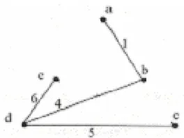
Theorem 4: If a subgraph of n-1 edges contains more than three nodes of degree more than one and if there is no pendent edge in the graph, the subgraph contains a circuit. Proof: For simplicity and easy to explain the theorem we consider a simple connected graph, shown in figure-1.
Form the given graph in figure 1, if we consider the edge combination, 1 4 5 6 2, the degree of each vertices corresponding to the given edge combination are,
1
3
1
3
1
e
d
c
b
a
Since there are three vertices of degree one and only
two vertices of degree more than one, hence this n-1 edges combination will not produce a tree of the graph G. The pictorial form of this tree is shown in figure 2.
Considering another example, if edge combination is, 0 3 5 6 2, of the graph shown in figure 1, the degree of each vertices corresponding to the given edges combination are,
3
2
2
1
1
e
d
c
b
a
Fig.1: A Simple Connected Graph
Node No. : Degree :
Fig. 2: An Illustrative Tree of Graph in Fig. 1
In the above combination two vertices of degree one and three vertices of degree more than one, hence this combination may give the circuit. Deleting pendent edges incidence on vertex a and b, the modified degree of all the vertices are,
2
2
2
0
0
e
d
c
b
a
Since, the degree of all the three vertices are more than one, this is confirm that the edge combination will produce a circuit. The pictorial form of this combination is shown in figure 3.
5. Circuits Testing Algorithm:
This algorithm ascertains us by testing whether n-1 edges combinations generated by “All Spanning Tree Generation Algorithm” are a circuit or not.
Step 1: From n-1 edges and incidence matrix obtain degree of each node contributed by n-1 edges under consideration. Step 2: Test whether at least two nodes of degree one? If not, go to step 6. Otherwise continue.
Step 3: test whether at least three nodes of degree more than one? If not go to step 5
Step 4: Delete pendant edges, if exists of n-1 edges and modify the degree of the nodes accordingly and go to step 2. Otherwise go to step 6.
Step 5: Edge combinations are tree. Step 6: Stop.
6. Complexity of the Proposed Algorithm:
The time complexity of the circuit testing remains same as the existing algorithms, however the new circuit testing algorithm is simple and easy to implement. The probability of generation of the circuit is very less in the new minimal spanning tree generation algorithm because we have always chosen an edge of the graph G, at least one end vertex of which is not yet colored. Obviously, time complexity of our algorithm is less than the existing algorithms due to removal of sorting of edges and finding the neighbor in every stage whose weight is minimal, of the constructed spanning tree. The space complexity of the algorithm is
(n.e)
where n is the number of vertices and e is number of edges of the graph G.7. Results and Conclusion:
Hardware used to carry out this experiment is Pentium IV computer and one GB DDR2 RAM. The program written in ‘C’ programming language and Turbo ‘C’ compiler used for compilation and execution purpose. The experiment has performed on several graphs of different types.
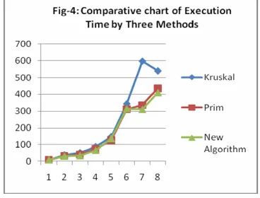
The storage requirement of this algorithm is proportional to (n x e). The experimental result of the algorithms is given in Table 1 and comparative chart of execution time of Kruskal, Prim and New Algorithm shown in the figure-4.
References:
[1]. A. Rakshit, A. K. Choudhury, S. S. Sarma and R. K. Sen, “An Efficient Tree Generation Algorithm,” IETE, vol. 27, pp. 105-109, 1981.
Node No. : Degree :
[2]. Sanjay Kumar Pal and Samar Sen Sarma, “An Efficient All Spanning Tree Generation Algorithm”, IJCS, vol. 2, No. 1, pp. 48 – 59, January 2008.
[3]. Sanjay Kumar Pal et. al., “Generation of Minimal Spanning Tree Based on Analytical Perspective of Degree Sequence”, Journal of Physical Science, Vol. 13, 2009. [4]. Kenneth Sorensen and Gerrit K. Janssens, “An Algorithm to Generate All Spanning Trees of a Graph in Order of Increasing Cost,” Pesquisa Operacional, vol. 25, pp. 219- 229, 2005.
[5]. N. Deo, “Graph Theory with Application to Engineering and Computer Sciences,” PHI, Englewood Cliffs, N. J, 2007.
[6]. Thomas H. Coremen, Charles E. Leiserson, Ronald L. Rivest, Clifford Stein, “Introduction to Algorithms”, PHI, Second Edition, 2008.
[7]. Harowitz Sahnai & Rajsekaran, “Fundamentals of Computer Algorithms”, Galgotia Publications Pvt. Ltd., 2000.
[8] Sanjoy Dasgupta, Christos Papadimitriou, Umesh Vazirani, “Algorithms”, Tata McGraw-Hill, First Edition, 2008
[9] http://ocw.mit.edu/NR/rdonlyres/Mathematics/18-310CFall-2007/LectureNotes/20_ln.pdf.
[10] R. J. Wilson, “History of Graph Theory”, Section 1.3, Handbook of Graph Theory, pp. 29 – 49, 2004.
AUTHORS BIOGRAPHY
Sanjay Kumar Pal
Completed degree in Mechanical Engineering and MCA. He has more than 18 years experience, 8 years in Engineering industry, 4 years in Software engineering, 6+ years in Academic institution. He has 20 National and international publication in the field of graph Theory and Network Topology Design.
Prof. Samar sen Sarma
Completed M.Tech. and Ph.D in Computer Sc. from Calcutta University. At present Sr. Professor of Calcutta University in the dept. Computer Sc. & Engineering. He has more than 150 research paper in national and international Journal.
Table1: Execution time of Kruskal, Prim and New algorithm
Execution Time of Algorithm * 100 (in Second)
No. of Node
No. of Edge
Kruskal Prim Algorithm New 3 3 1.70 1.95 1.76 4 4 4.56 4.46 3.51 4 5 4.67 4.72 3.57 5 8 7.36 7.42 5.94 6 12 8.84 8.90 8.90 7 13 18.78 16.75 12.52 7 17 19.12 20.59 16.22 8 25 18.89 18.89 18.80 9 21 24.44 21.75 21.61 9 32 37.35 31.69 29.88 10 18 33.28 32.76 30.42 10 42 38.66 36.80 32.72 11 27 36.80 36.74 33.40 11 50 40.18 37.56 37.26 12 20 36.68 37.14 36.32 12 53 51.30 40.32 32.84 13 31 73.60 51.74 47.68 13 70 79.94 55.03 57.68 14 55 71.94 67.87 70.83
14 82 124.68 120.20 122.70
15 32 87.60 73.68 64.50
15 72 121.65 101.85 105.95
16 48 98.25 74.35 73.60 16 108 123.70 118.65 102.35
17 41 121.40 109.30 102.35
17 55 144.75 124.55 120.25
18 76 146.35 125.85 136.10
19 68 177.95 156.80 128.90
20 95 317.60 231.81 315.40
21 74 343.80 312.60 315.60
22 69 530.6 292.2 269.4 23 126 596.40 336.63 310.64
24 82 561.22 441.02 420.15
25 78 540.34 434.77 410.23