A Naïve Bayes Model using Semi-Supervised Parameters for Enhancing the Performance of Text Analytics

A Naïve Bayes Model using Semi-Supervised

Parameters for Enhancing the Performance of

Text Analytics

K. Rajarajeshwari1

Research Scholar, Department of Computer Science, Dr.G.R.Damodaran College of Science, Coimbatore-14 Email: [email protected]

Dr. G. Radhamani2

Director, Department of Computer Science, Dr.G.R.Damodaran College of Science, Coimbatore-14

---ABSTRACT---Sentiment mining is an emerging area that utilizes the feedback of the users to make intelligent decisions in marketing. Consumer reviews helps the user to convert oral conversations to digital versions to be used in marketing analytics. Since e-commerce takes intrinsic forms in present day business, the need to get positive reviews for specific products is vital on an organization perspective. Both sentiment mining and TF-IDF (Term Frequency-Inverse Document Frequency) are text mining tasks but have their unique applications and characteristics. Sentiment mining classifies the documents into positive, negative or neutral opinions that are used to derive intelligent decisions. TF-IDF classifies the documents into sub-categories within the documents itself. Utilizing the TF-IDF as a feature for sentiment mining improves the performance of classification. In this research work a strategy is applied for feature preprocessing to evaluate the consumer’s sentiments accurately. This strategy makes use of the semi-supervised parameter estimation Naïve Bayes Model. The experimental results demonstrate that TF-IDF tuning approach results in better optimized results.

Keywords – Sentiment Analysis, e-commerce, Naïve-Bayes Model, Text Mining.

--- --- Date of Submission: April 26, 2019 Date of Acceptance: May 09, 2019 ---

---I.

INTRODUCTION

B

usiness in present day scenario cannot be performed neglecting the social media. Facebook, Twitter, YouTube and Whatsapp are used to reach the customers to promote the new brands by many of the companies. Some products are sold only through online mode only. CoolPad cell phone might be an example for selling through online alone. No retail or selling point is available for purchasing the phone. Rather the phone can only be purchased through online mode. This was a strong connotation for the power of e-commerce.

Online consumer reviews present in internet is as important as getting good sales promoters for the product. Nielson study shows that online consumer reviews are the second most-trusted source of product information after recommendations from family and friends. Since the importances have hiked, the attentions towards the social media have increased.

The research hypothesis laid in this paper is:

H1: “Utilizing the TF-IDF Feature interpretation in Semi-Supervised parameter estimation Naïve Bayes Model in Sentiment Mining of Online Consumer Reviews (OCR) would improve the performance”

The organization of the paper subsequently tries to substantiate the assumption:

The paper is organized as follows: Literature review is given in Section II, followed by the problem definition of the sentiment mining, TF-IDF and Naïve Bayes in next section. Section IV documents the technical perspectives of the working method deployed in this experiment. In

Section V, results are explained followed by discussion. Section VII presents the conclusion of the paper.

II.

RELATED

WORK

The positive or negative impression about an aspect of a sentiment holder is termed as sentiment. There are different orientations for sentiments as positive, negative, or neutral.

These are also termed as polarities of the opinion. Opinion mining is very broad area that could be classified as [1]:

1. Document Level: This classifies a whole document into two sentiments as either positive or negative. In this category, it is assumed that each document conveys sentiments on one attribute [2].

2. Sentence Level: This ensures if each sentence denotes a neutral opinion in addition to the common positive and negative opinions for a product or service. This method makes a clear demarcation between objective and subjective sentences. The objective sentences represent genuine information. The subjective sentence represents opinions that are subjective in nature. Generally, the objective sentences represent more opinions than the subjective sentences [2].

3. Entity and Aspect level: Opinion mining that is based on feature and its summarization is termed as Aspect level analysis. This produces results in a finer granularity. The foundation of this is the concept that an opinion could hold either a positive or negative sentiment or a target of that opinion [3].

opinions. A sentiment expressed only on a particular entity or an aspect of the entity is a regular opinion. A sentiment expressed by comparing multiple aspects based on some of their shared attributes is a comparative opinion [4].

For e.g., “Vanilla pastries taste better than vanilla cake”, compares pastries and cake based on their tastes (an aspect) and expresses feeling and preference for pastries. Sentiment classification is extremely responsive to the area from which the training data are extracted. This makes it an interesting research topic which transfers learning or domain adaptation.

Words and even language formats used in different areas for expressing sentiments can be somewhat different hence a classifier trained using opinionated documents from one area often performs differently from another area when it is tested or applied on opinionated documents.

The same word in one area may mean positive, but in another contextual area may mean negative, making matters difficult. Thus, domain modification is needed. It is found that existing research has used labeled data class from one area, unlabelled data class from the target area and general opinion words as features for adaptation [5, 6, 7, 8]. The applications for sentiment analysis in research pertaining to academics are endless. Software called SentiStrength is deployed for analysing academic research in existing works [12, 14]. Ghose proposed a method to improve the usefulness of the review by converting it into votes cast by the reader [13].

Thousands of text documents can be processed for sentiment (and other features including named entities, topics, themes, etc.) in seconds, compared to the hours it would take a team of people to process the same manually. Many businesses are adopting text and sentiment analysis and incorporating it into their processes because of its efficiency and accuracy.

The goal of text classification is to assign some piece of text to one or more predefined classes or categories. Sentiment classification is a task of classifying whether the sentiments of text are positive or negative. Different Machine Learning and Lexicon approaches are used for sentiment analysis. Statistical Techniques for sentiment analysis are more popular. These techniques are based on Term Presence and Term Frequency. Some work instigates the usage of the n-gram features for the machine learning. The proposed working method of the research instigates the utilization of the TF-IDF and N-gram Features for the sentiment mining. The dataset once prepared will be subject to the machine learning technique which may be suitable for the text classification. WEKA toolkit is deployed for the experiments carried out in this paper.

III.

TEXT

MINING

AND

CLASSIFICATION

MODEL

3.1 SENTIMENT MINING

Sentiment mining is the exploration of data mining techniques for the “voice of consumer” data such as reviews, posts, tags and articles. Sentiment analysis deals with use of text analysis, natural language processing and

computational linguistics to systematically extract, interfere and study the customer attitude.

Stumble on the overall contextual polarity or emotion is the ultimate of the sentiment mining. A basic task in sentiment analysis is classifying the polarity of a given text at the document, sentence, or feature/aspect level— whether the expressed opinion in a document, a sentence or an entity feature/aspect is positive, negative, or neutral. Advanced, "beyond polarity" sentiment classification looks, for instance, at emotional states such as "angry", "sad", and "happy".

3.2 TF-IDF

TF-IDF (Term Frequency-Inverse Document Frequency) is a text mining technique used to categorize documents. TF-IDF computes a weight which represents the importance of a term inside a document. It does this by comparing the frequency of usage inside an individual document as opposed to the entire data set (a collection of documents).

The importance increases proportionally to the number of times a word appears in the individual document itself--this is called Term Frequency. However, if multiple documents contain the same word many times then you run into a problem. That's why TF-IDF also offsets this value by the frequency of the term in the entire document set, a value called Inverse Document Frequency.

𝑇𝐹 (𝑡) =𝑁𝑜. 𝑜𝑓𝑡𝑖𝑚𝑒𝑠 𝑡𝑒𝑟𝑚, 𝑡 𝑎𝑝𝑝𝑒𝑟𝑠 𝑖𝑛 𝑡ℎ𝑒 𝑑𝑜𝑐𝑢𝑚𝑒𝑛𝑡, 𝐷_{𝑇𝑜𝑡𝑎𝑙 𝑛𝑢𝑚𝑏𝑒𝑟 𝑜𝑓 𝑡𝑒𝑟𝑚𝑠 𝑖𝑛 𝑡ℎ𝑒 𝑑𝑜𝑐𝑢𝑚𝑒𝑛𝑡, 𝐷}

𝐼𝐷𝐹 (𝑡) =_{𝑁𝑢𝑚𝑏𝑒𝑟 𝑜𝑓 𝑑𝑜𝑐𝑢𝑚𝑒𝑛𝑡𝑠 𝑤𝑖𝑡ℎ 𝑡𝑒𝑟𝑚 𝑡 𝑖𝑛 𝑖𝑡}log 𝑒 ( 𝑇𝑜𝑡𝑎𝑙 𝑛𝑢𝑚𝑏𝑒𝑟 𝑜𝑓 𝑑𝑜𝑐𝑢𝑚𝑒𝑛𝑡𝑠)

𝑇𝐹 − 𝐼𝐷𝐹 = 𝑇𝐹(𝑡) ∗ 𝐼𝐷𝐹(𝑡)

TF-IDF is computed for each term in each document. Typically, you will be interested either in one term in particular (like a search engine), or you would be interested in the terms with the highest TF-IDF in a specific document (such as generating tags for blog posts).

TF-IDF Algorithm with Illustration

Step 1: Score Generation

Suppose the customer review has 100 word with the word "good" in it 5 times.

a. The calculation for the Term Frequency would be:

TF(t) = 5/100 = 0.05

Next, assume the entire collection of review posts has 10,000 documents and the word "good" appears at least once in 100 of these.

b. The Inverse Document Frequency calculation would look like this:

IDF(t) = log(10,000/100) = 2

c. To calculate the TF-IDF, multiply the previous two values. This gives us the final score:

Step 2: Decide a Threshold to Tag

After running this Score Generation against all 100 of the Twitter tags with the word "Good", now end up with a score for each. Let's assume that the document have a wide range of scores, ranging from 0.05 to 0.5.

Continuing a simple example from this collection, 0.05 would be a 100 word document with 1 instance of "Good" and 0.5 would be a 100 word document with "Good" appearing 25 times. To determine if the document will be tagged with "Good", decide on a threshold score.

The score chosen will vary depending on data set. A document with only one instance of "Good" (score 0.05) is unlikely to be focused on “Good”, but obviously the high score of 0.5 is probably on topic.

3.3 Naïve Bayes

Naive Bayes classifiers, a family of classifiers that are based on the popular Bayes’ probability theorem, are known for creating simple yet well performing models, especially in the fields of document classification and disease prediction.

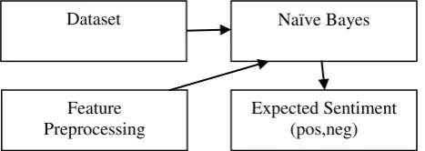
Figure 1: Overall Working Method of the System

Proposed Semi-supervised parameter estimation Naïve Bayes Model

The proposed strategy is using the semi-supervised version of the Naïve Bayes model for the sentiment classification in online consumer review. Using the mixture model data with labeled and unlabelled instances, train the Naïve Bayes model and the steps involved are exemplified below:

Step 1: Given a collection D=L⨄U of labeled samples L and unlabeled samples U, start by training a naive Bayes classifier on L.

Until convergence, do:

Step 2: Consider the problem of classifying Online Consumer Review (OCR) by their link based features, into positive and negative. Probability that the ith feature of a given review occurs in a feature set, w from class C can be written as:

Then the probability that a given Document D contains all of the features , given a class C, is

𝑝(𝐷|𝐶) = ∏ 𝑝(𝑤𝑖|𝐶) 𝑖

Step 3: The goal is to find: "what is the probability that a given OCR Document, D belongs to a given class C?" which is defined as:

𝑝(𝐷|𝐶) = 𝑝 (𝐷 ∩ 𝐶)_{𝑝 (𝐶)}

Predict class probabilities P(C│x)for all examples x in D. Step 4: Bayes' theorem manipulates the statement of probability in terms of likelihood.

𝑝(𝐶|𝐷) = 𝑝 (𝐶)_{𝑝 (𝐷) 𝑝}(𝐷|𝐶)

Step 5: OCR document classification has only two

mutually exclusive classes, S and ¬S (positive and negative), such that every element (OCR document) is in either one or the other

𝑝(𝐷|𝑆) = ∏ 𝑝(𝑤𝑖 𝑖|𝑆) and 𝑝(𝐷|¬𝑆) = ∏ 𝑝(𝑤𝑖 𝑖|¬𝑆)

Using the Bayesian result above, it can be written as: 𝑝(𝑆|𝐷) = _{𝑝 (𝐷) ∏ 𝑝}𝑝 (𝑆) (𝑤𝑖|𝑆)

𝑖 Dividing one by the

𝑝(¬𝑆|𝐷) = 𝑝 (¬𝑆)_{𝑝 (𝐷) ∏ 𝑝}(𝑤𝑖|¬𝑆) 𝑖

which can be re-factored as:

_{𝑝 (¬𝑆|𝐷) =} 𝑝 (𝑆|𝐷) _{𝑝 (¬𝑆) ∏}𝑝 (𝑆) _{𝑝 (𝑤}𝑝 (𝑤𝑖|𝑆) 𝑖|¬𝑆) 𝑖

Thus, the probability ratio p(S | D) / p(¬S | D) can be expressed in terms of a series of likelihood ratios.

Step 6: The actual probability p(S | D) can be easily computed from log (p(S | D) / p(¬S | D)) based on the observation that p(S | D) + p(¬S | D) = 1. Taking the logarithm of all these ratios, it is possible to obtain the results:

𝑙𝑛_{𝑝 (¬𝑆|𝐷)}𝑝 (𝑆|𝐷) = 𝑙𝑛 _{𝑝 (¬𝑆)}𝑝 (𝑆) + ∑ 𝑙𝑛 𝑝 (𝑤𝑖|𝑆)

𝑝 (𝑤𝑖|¬𝑆)

𝑖

Finally, the Sentiment can be classified as follows. It is positive if 𝑝 (𝑆|𝐷) > 𝑝 (¬𝑆|𝐷) (i.e., 𝑙𝑛 𝑝 (𝑆|𝐷)

𝑝 (¬𝑆|𝐷) > 0), otherwise it is negative.

Step 7: Re-train the model based on the probabilities (not the labels) predicted in the previous step.

Step 8: Convergence is determined based on improvement to the model likelihood P(D│θ), where θ denotes the parameters of the naive Bayes model.

This training algorithm is an instance of the more general expectation–maximization algorithm (EM): the prediction step inside the loop is the E-step of EM, while the re-training of naive Bayes is the M-step. The algorithm is formally justified by the assumption that the data are generated by a mixture model, and the components of this mixture model are exactly the classes of the classification problem.

IV.

T

ECHNICAL

P

ERSPECTIVES OF WORKING

M

ETHODOLOGY

4.1 DATASET

The dataset compiled with data of online consumer review regarding the product “Apple iPod” is collected from the Twitter from June 2017 to July 2017. Among the samples, 300 were preprocessed and selected.

Naïve Bayes

Feature Preprocessing

Dataset

The text preprocessing for training set includes removal of special characters such as #, !, @. Then the text is manually reviewed and sentiment is classified.

The dataset is collected from the twitter and each instance in the data set has 2 fields:

• sentiment_label - the polarity of the tweet (pos, neg) • tweet_text - the text of the tweet

4.2 METHODOLOGY

Initially the dataset is collected as mentioned in above section. The file with “StringtoWord” preprocessing will look like Figure 2.

Figure 2: Experiment Dataset View

Figure 3: Dataset with “StringtoWord” Text Preproceesing (Two Classes (Blue:Positive,

Red:Negative))

Next to that, the compiled dataset is converted into arff file by applying the “StringtoWordVector” option. Now the words present in the dataset will be converted into bag of words format.

Figure 4: Dataset tuned for TF-TDF

Now the Naïve Bayesian Classifier is deployed for the dataset, results are recorded.

The bag-of-words vector representation model is commonly used for text classification. In this method, the frequency of occurrence of each word, or term-frequency (TF), is multiplied by the inverse document frequency, and the TF-IDF scores are used as feature values for training a classifier. TF-IDF options are enabled and the dataset would again get subject to alterations. This will make the dataset to bag of words model. Now the dataset would look like Figure 6.

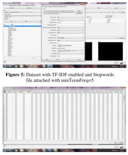
Figure 5: Dataset with TF-IDF enabled and Stopwords file attached with minTermFreq=5

Figure 6: Dataset Values view after Preprocessing Now the dataset will be subject to again the Naïve bayesian classifier and the results will be recorded. Now the stop words removal will be done with the data file “stopwords-eng.txt”(Figure 7). The file will be attached with the dataset and minTermFrequency will be modified to 5 and one execution will be done. Results are recorded.

V.

E

XPERIMENTAL

R

ESULTS

Class for a Naïve Bayes classifier using estimator classes. Numeric estimator precision values are chosen based on analysis of the training data. For this reason, the classifier is not an UpdateableClassifier (which in typical usage are initialized with zero training instances) -- if you need the UpdateableClassifier functionality, use the NaiveBayesUpdateable classifier. The NaiveBayesUpdateable classifier will use a default precision of 0.1 for numeric attributes when buildClassifier is called with zero training instances.

OPTIONS

debug -- If set to true, classifier may output additional info to the console.

displayModelInOldFormat -- Use old format for model output. The old format is better when there are many class values. The new format is better when there are fewer classes and many attributes.

useKernelEstimator -- Use a kernel estimator for numeric attributes rather than a normal distribution.

useSupervisedDiscretization -- Use supervised discretization to convert numeric attributes to nominal ones.

Three datasets are used in the experiments and their technical aspects are as follows:

Base dataset – compiled dataset with “StringToWord” feature preprocessing.

FP-1 – compiled dataset with “StringToWord” feature preprocessing+uses the TF-IDF transformation

FP-2 - compiled dataset with “StringToWord” feature preprocessing+uses the TF-IDF

transformation+StopWords removal+minTermFrequency – 5

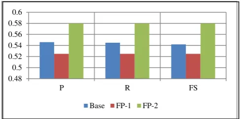
The classifier is evaluated in six different datasets with different sample sizes. Results of the three feature processing datasets are portrayed in Figure 8, 9 and 10. Figure 8 depicts the time taken for the evaluation. It is clearly evident that the feature processing decreases significant time. Figure 9 compares the correctly and incorrectly classified instances. Figure 10 depicts performance comparison of the datasets (Precision, Recall and F-Score).

Figure 8: Time Taken for the execution of proposed classifier in different datasets

Figure 8 represents the time taken for the execution of the proposed algorithm for three different datasets. The proposed algorithm is first deployed in the base dataset which is represented as “BASE” in the graph. Then feature processing is deployed in the BASE dataset.

FP-1 is attained through String to Word conversion and TF-IDF transformation. FP-2 is attained through subjecting the FP-1 to stopword removal process and mintermfrequency process. It is evident that when all two - fold preprocessing is done the time taken is considerable reduced.

Figure 9: Correctly (CC) Vs. Incorrectly (IC) classified instances

Figure 9 represents the correctly and incorrectly classified samples for the proposed method in three different dataset.

Figure 10: Precision (P), Recall(R) and F-Score of the proposed classifier on different datasets

The precision, recall and F-Score of the proposed method in three different dataset (BASE, FP-1, FP-2) are depicted in Figure 10.

Figure 11: ROC Value of the proposed classifier on datasets

0 0.1 0.2 0.3

BASE FP-1 FP-2

Time

Time Expon. (Time)

0 20 40 60 80

Base FP-1 FP-2

CC IC

0.48 0.5 0.52 0.54 0.56 0.58 0.6

P R FS

Base FP-1 FP-2

0.5 0.55 0.6

BASE FP-1 FP-2

ROC

The Receiver Operating Characteristic (ROC) curve for the proposed method at three different dataset (BASE, FP-1, FP-2) are depicted in Figure 10.

VI.

D

ISCUSSION

The dataset is run for three different sample sizes (100, 200 and 300). The results recorded are subject to the statistical Paired T-Test for proving the hypothesis stated in Section I. Justification for this approach is given through the statistical measure two-tailed paired t-test.

The t test compares one variable between two groups. It is suggested to compare a continuous variable. It is often used to compare “before” and “after” scores in experiments to determine whether significant change has occurred. In this research work, the problem taken is, to find that the concept feature weight is necessary for the domain-centric approach.

Formula: t =(x ̅-μ)/(s/√n)

Where x̅ is the mean of the change scores, μ is the hypothesized difference (0 if testing for equal means), s is the sample standard deviation of the differences, and n is the sample size. The number of degrees of freedom for the problem is n – 1. Implementation part is given in Table 3.7.

In paired sample hypothesis testing, a sample from the population is chosen and two measurements for each element in the sample are taken. Each set of measurements is considered a sample. Paired samples are also called matched samples or repeated measures. The advantage of this approach is, the sample can be smaller and is not affected by any external factor. A paired t-test looks at the difference between paired values in two samples, takes into account the variation of values within each sample, and produces a single number known as t-value. Two tailed tests are used when the user has no idea which sample will be larger than the other. Two-tailed test evaluates whether a difference exists between two samples, but not the direction of the difference. The hypothesis of the paper is H1 which was tested against the null hypothesis.

Table 1: Paired T-Test Results of the Proposed Method

Samples No-FP FP

100 52.3 57.1

200 53.6 56.2

300 56.4 59.3

Average Variable 1 57.533

Average Variable 2 54.100

Standard error Variable 1 0.921

Standard error Variable 2 1.210

P value 0.038

Alternative hypothesis: Ha : μ ≠0

H1: “Utilizing the TF-IDF Feature interpretation in Semi-Supervised parameter estimation Naïve Bayes Model in Sentiment Mining of Online Consumer Reviews (OCR) would improve the performance”

The null hypothesis: H0: μ = 0

H0: “Utilizing the TF-IDF Feature interpretation in Semi-Supervised parameter estimation Naïve Bayes Model in Sentiment Mining of Online Consumer Reviews (OCR) would doesn’t have any improvement in the performance” Is the p value less than 0.05?

 If no, then the averages are not significantly different (cannot reject null hypothesis)

 If yes, then the averages are significantly different (accept an alternative hypothesis) The P-Value 0.038 is less than the 0.05, so the null hypothesis is rejected at 95 % confidence. The test has provided evidence that the proposed Semi-supervised Parameter Estimation Naïve Bayes is efficient for the Sentiment Mining in Online Consumer Review.

VII.

C

ONCLUSION

The applications of sentiment mining could be used comprehensively by organizations in their decision making process. These decisions mainly pertain to the marketing of products of an organization. Considering the significance of consumer reviews, it is always important to get good feedback about the products that a company decides to sell. The paper illustrates how TF-IDF and sentiment mining could be used simultaneously to improve classification and derive useful information. The concept of feature preprocessing is used to analyze the sentiments of the consumer exactly. The fundamental concept used in the paper is a Naïve Bayes Model that uses semi-supervised parameter estimation. The experimental results substantiate the fact that the TF-IDF approach ends up with better results.

REFERENCES

[1] Asha S Manek, P Deepa Shenoy, M Chandra Mohan,•Venugopal K R, Aspect term extraction for sentiment analysis in large movie reviews using Gini Index feature selection method and SVM classifier, World Wide Web, Springer Science+Business Media New York 2016

[2] Liu, B.: Sentiment Analysis and Opinion Mining, p. 7. Morgan and Claypool Publishers, USA (2012)

[3] Hu, M., Liu, B.: Mining and Summarizing Customer Reviews. In: Proceedings of the tenth ACM SIGKDD international conference on Knowledge Discovery and

Data Mining (168–177). ACM (2004)

[4] Jindal, N., Liu, B.: Mining comparative sentences and relations. In AAAI 22, 1331–1336 (2006)

Proceedings of Recent Advances in Natural Language Processing (RANLP-2005) (2005)

[6] Blitzer, J., Dredze, M., Pereira, F.: Biographies, Bollywood, Boomboxes and Blenders: Domain Adaptation for Sentiment Classification. In: Proceedings of Annual Meeting of the Association for Computational Linguistics (ACL-2007) (2007)

[7] Pan, S., Ni, X., Sun, J., Yang, Q., Chen, Z.: Cross-domain Sentiment Classification via Spectral Feature Alignment. In: Proceedings of International Conference on World Wide Web (WWW-2010) (2010)

[8] Yang, H., Si, L., Callan, J.: Knowledge Transfer and Opinion Detection in the TREC2006 Blog Track. In: Proceedings of TREC (2006)

[9] George H. John, Pat Langley: Estimating Continuous Distributions in Bayesian Classifiers. In: Eleventh Conference on Uncertainty in Artificial Intelligence, San Mateo, 338-345, 1995.

[10] https://en.wikipedia.org/wiki/Sentiment_analysis [11] Twitter. https://twitter.com/Twitter

[12] Garcia, D., and Schweitzer, F., 2011. "Emotions in Product Reviews-Empirics and Models,"2011 IEEE International Conference on Privacy, Security, Risk, and Trust, and IEEE International Conference on Social Computing, IEEE, pp. 483-488.

[13] Ghose, A., and Ipeirotis, P.G. 2011. "Estimating the helpfulness and economic impact of product reviews: Mining text and reviewer characteristics," IEEE Transactions on Knowledge and Data Engineering (23:10), pp 1498-1512.

[14] Gruzd, A., Doiron, S., and Mai, P., 2011. "Is happiness contagious online? A case of Twitter and the 2010 Winter Olympics," Proceedings of the 44th Hawaii International Conference on System Sciences, IEEE, pp. 1-9.

[15] Xiaojiang Lei, Xueming Qian, Member, and Guoshuai Zhao, Rating Prediction based on Social Sentiment from Textual Reviews, IEEE Transactions on Multimedia (Volume: 18, Issue: 9, Sept. 2016).

[16] Oscar Araque, Ignacio Corcuera-Platas, J. Fernando Sánchez-Rada, Carlos A. Iglesias, Enhancing deep learning sentiment analysis with ensemble techniques in social applications, Elsevier, Expert Systems With Applications 77 (2017) 236–246.

[17] Zhen Hai, Gao Cong, Kuiyu Chang, Peng Cheng, and Chunyan Miao, Analyzing Sentiments in One Go: A Supervised Joint Topic Modeling Approach, IEEE Transactions on Knowledge and Data Engineering, vol. 29, no. 6, June 2017.

[18] Jasleen Kau , Dr.Jatinderkumar, R. Saini, An Analysis of Opinion Mining Research Works Based on Language, Writing Style and Feature Selection Parameters, Int. J. Advanced Networking and Applications, ISSN: 0975-0290, 2014.

[19] Mahalakshmi R, Dr. M. Nandhini and Kowsalya G, Sentimental Analysis for Social Media – A Review, Int. J. Advanced Networking and Applications, Volume: 10 Issue: 03 Pages: 3860-3863 (2018) ISSN: 0975-0290. [20] Lakshmi. K, Harshitha.K.Rao, Revathi. V, Mrinal, Archana.T.P, Emotion Recognition: Detecting Emotions

from Textual Documents, Blogs and Audio Files, Int. J.Advanced Networking and Applications, ISSN: 0975-0282.

Appendix – A Sample Dataset

Database description @relation 'ipod

- weka.filters.unsupervised.attribute.StringToWordVector-

R-W1000-prune-rate-1.0-N0-

stemmerweka.core.stemmers.NullStemmer-M1-tokenizerweka.core.tokenizers.WordTokenizer -delimiters @attribute Sentiment {neg,pos}

@attribute 'Tweet Content'

{ pos, 'I love this ipod except for the battery life '} { pos, ' long battery scratch resistant'}

{neg, ' Battery drains even if I don t use it '}

{ pos, ' great in the car light portable good quality long battery scratch resistant '}

{ pos, '5G lies a more mature iPod many steps wiser and more able than its one year old The iPod gains many incremental improvements including a brighter screen and better video battery life but probably the most appealing aspect is the tantalizing price points of $249 for the 30GB version and $349 for the huge 80GB version '} { pos, '5GB and the better battery life rated for up to 6 '} {neg, ' The battery doesn t last a long time especially when you re recording or watching a video but I just listen to music most of the time and it lasts me a good length of time doing that '}