Performance Comparison of Various Noisy Audio
Signals Analysis Using Different Sampling Rates
Dr.P.Kannan
Professor, ECE Department, PET Engineering College, Vallioor, Tamilnadu, India. [email protected]
G.Bharatha Sreeja
2
Assistant Professor, ECE Department, PET Engineering College, Vallioor, Tamilnadu, India. [email protected]
J. Hermus Mary Shifani
PG Scholar, Communication Systems, PET Engineering College, Vallioor, Tamilnadu, India.
---ABSTRACT ---The discrete time systems that process data at more than one sampling rate are known as multirate systems. ---The two basic operations in multirate signal processing are decimation and interpolation.One of the important applications of multirate signal processing is sub-band coding of speech signal. In the proposed system, speech signal is taken as input signal. Additive White Gaussian Noise is added with the input speech signal. The input speech signal spectrum is divided into frequency sub-bands using a bank of finite response filters. Hamming, Hanning, Blackman, Rectangular and Kaiser windowing methods are used to implement the low pass and high pass filters. Finally performance of the proposed system is evaluated on the TIMIT data base using the parameters like leakage factor, main lobe width, side lobe attenuation, peak amplitude of side lobe and signal to noise ratio. The performance evaluation shows which window is suitable for designing the finite impulse response filters and sub-band coding system.
Keywords - Windowing, Signal to Noise Ratio, FIR Filter, Multirate.
--- --- Date of Submission: Feb 10, 2018 Date of Acceptance: March 07, 2018 --- ---
I.
INTRODUCTIONM
ultirate means multiple sampling rates. A multirate digital signal processing system uses multiple sampling rates among the system. Whenever a signal at one sampling rate has to be used by a system that expects a different sampling rate, the rate has to be increased or decreased, and some processing is required to do so. Therefore multirate digital signal processing refers to art or science of changing the sampling rates. Systems that use multiple sampling rates in the processing of digital signals are called multirate digital signal processing systems. In telecommunication systems that transmits and receives different kinds of signals as an example teletype, facsimile, speech, video, etc., there is a requirement to process the various signals at different rates. The processing of converting a signal from a given rate to a different rate is called sampling rate conversion.Multirate digital signal processing systems use a down sampler and an up sampler. The two primary operations that enable the data rate to be altered in an efficient manner are decimation and interpolation. Decimation reduces the sampling rate, effectively compressing the information, and retaining only the required data. Interpolation on the other hand increases the sampling rate of the information subsequently. Multirate signal processing finds its applications in many fields like speech and audio processing, communication systems, antenna systems, radar systems, A/D, D/A converters, sub band coding, voice privacy using analog phone lines etc. During decimation process the sampling rate is reduced from Fs to
Fs/M by deleting M-1 samples for every M samples within the original sequence. Interpolation works by inserting L-1 zero-valued samples for every input sample. The sampling rate thus increases from Fs to LFs.
II.LITERATURE SURVEY
Ashraf M. Aziz (2009) proposed a structure of two channel Quadrature Mirror Filter (QMF) with low pass, high pass filters, decimators and interpolators to perform sub-band coding of speech signals in advanced area. The execution of the proposed structure is contrasted with the execution of the delta-modulation encoding systems. The outcomes demonstrate that the proposed structure essentially diminishes the mistake and accomplishes significant execution change contrasted with delta-modulation encoding systems. Maurya A.K. and Deepak Nagaria (2011) exhibited decimation and interpolation procedures of multirate signal processing which are rate change methods. The favourable position is interpolation can change the sampling rate of the signal without changing its unique substance.
permits complete disposal of amplitude and phase distortion of the recreated signal. The remade signal is contrasted with the original input speech signal.
Dolly Agrawal and Divya Kumud (2014) presented multirate signal processing methods, for example, decimation and interpolation by integer factors and after that exhibited how the two procedures can be joined to acquire sampling rate change by any rational component. The impediment of this paper is that the impacts of aliasing for decimation and pseudo images for interpolation are made while designing the multirate systems. Prajoy Podder, Tanvir Zaman Khan, M.Muktadia Rahman and Mamdudul Haque Khan (2014) proposed windowing systems for the comparison of execution of Hamming, Hanning and Blackman window based on their magnitude response, phase response and equivalent noise bandwidth. Looking simulation consequences of various window, Blackman window has best execution among them and the response of the Blackman window are more smooth and perfect. The fundamental downside is that the Blackman window has higher equivalent noise bandwidth. Jagriti Saini and Rajesh Mehra (2015) displayed comparative examination of speech signal utilizing different windowing methods such as Hamming, Hanning and Blackman window. It can be gotten from the reproduced results that the Blackman window contains almost double power when contrasted with Hamming and Hanning window. So for long distance communication Blackman window is utilized. Suresh Babu, D.Srinivasulu Reddy and P.V.N.Reddy (2015) utilized windowing techniques and the execution of Hamming, Hanning and Blackman windows are mainly compared depending on their magnitude response, phase response. In this paper, on
looking at the simulation results utilizing different windows, we watched that Blackman window creates better results among them.
Lalima Singh (2015) built up speech signal analysis strategy taking into account Fast Fourier Transform (FFT) and Linear Predictive Coding (LPC). These techniques are utilized to extract and compress a few elements of the speech signal. The primary restriction of this paper is that the spectrum investigation is complex procedure of breaking down the speech signal into comparative parts. Lalitha R. Naik and Devaraja Naik R L (2015) exhibited a low rate speech coder taking into account sub-band coding technique. This paper mainly focusing the comparison of correlation values for various clean speech signals and correlation values for in the wakenals at more than one of adding high amplitude noise to the same speech signals. Taking correlation tests demonstrate that its execution is fulfilling.
III.METHODOLOGY
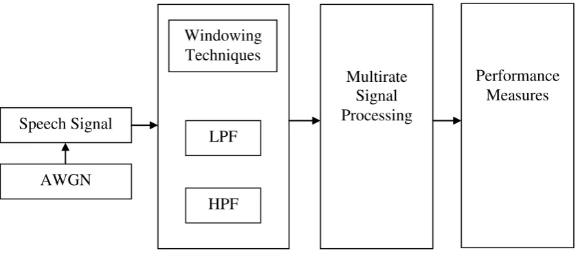
Speech signal is taken as the input signal. AWGN is added with the input speech signal. The finite impulse response filters are designed and implemented using different window function. Window function is a mathematical function that is zero-valued outside of some picked interval. When another function is multiplied by a window function, the product is also zero-valued outside the interval. LPF and HPF are designed using Rectangular, Hanning, Hamming, Blackman and Kaiser windows. Then multirate signal processing is performed Finally performance of the proposed system is evaluated based on main lobe width, leakage factor, side lobe attenuation, peak amplitude of side lobe and Signal to Noise Ratio.
Fig 3.1 Block diagram of proposed method
Speech Signal
Multirate
Signal
Processing
Performance
Measures
Windowing
Techniques
LPF
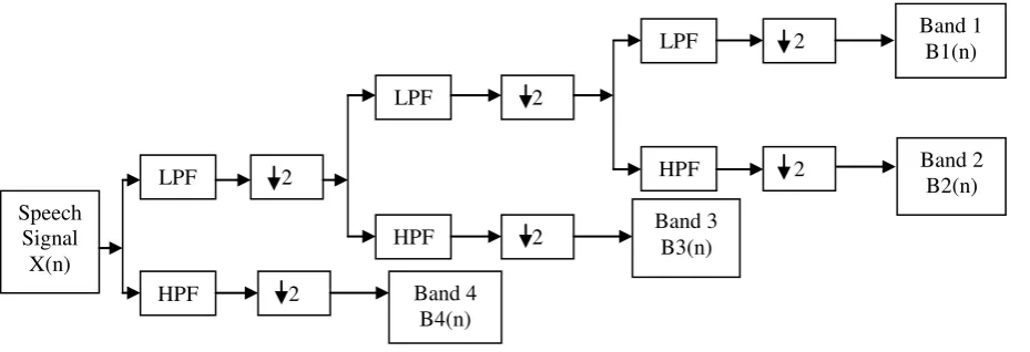
Fig 3.2 Speech signal sub band coding The above Fig 3.2 shows speech signal sub band coding
which has three frequency subdivision. Sub-band coding is a method where the speech signal is subdivided into several frequency bands and each band is digitally encoded separately. The primary frequency subdivision splits the input speech signal into two equal parts, a low pass signal and a high pass signal. Here the low pass signal from the primary stage is divided into two equal bands, a low pass signal and high pass signal. Here the signal is totally divided into four frequency bands. After the frequency subdivision, decimation by a factor of ‘2’ is performed.
3.1 FILTER DESIGN USING FIR
FIR filter means Finite Impulse Response digital filter. This filter has linear phase. It is relatively easy to design and highly stable. This filter is mostly used in different digital signal processing applications. The output can be obtained by [27], [28],
= ∑
𝑁−ℎ
−
= (1) Where,
is the input signal.
ℎ
is the impulse response of FIR filter.The z-transform of impulse response of FIR
filter
ℎ
is obtained by taking the transfer
function of a causal FIR filter [27], [28],
= ∑
𝑁−ℎ
= − (2)
3.1.1 Low Pass Filter
For the low pass filter the impulse response is given by [27], [28],
ℎ
= {
sin wcn
nπ
; n ≠
𝑤𝑐𝜋
; =
(3)
3.1.2 High Pass Filter
For the high pass filter the impulse response is given by the equation [27], [28],
ℎ
= {
− sin 𝑤𝑐
𝜋
; ≠
−
𝑤𝑐𝜋
; =
(4)
3.2 WINDOWING METHODS
A simple and efficient way to design an FIR filter is window method. A window is a finite array consisting of coefficients selected to satisfy the desirable requirements. While designing the finite impulse response filter using windowing method it is necessary to specify a window function to be used and the filter order according to the required specifications. These two requirements are interrelated. Each function is a kind of compromise between the two following requirements i.e. the higher the selectivity the narrower the transition region and the higher suppression of undesirable spectrum the higher the stop band attenuation. The main aim of a window function is to provide accurate type of responses with reduced side lobes and comparatively less pass-band and stop-band ripples. The Window method is the most popular and effective method because this method is simple, convenient, fast and easy to understand.
3.2.1 Rectangular Window
The rectangular window is expressed by using the below forumula which is given by,
= { ; ≤ ≤ 𝑁 −
; ℎ
𝑖
(5) Where,𝑁
is the order of the filter.Band 1 B1(n)
Band 2 B2(n) Band 3
B3(n) Band 4
B4(n) Speech
Signal X(n)
HPF LPF
HPF
2
2
LPF 2
2
LPF
HPF
2
3.2.2 Hanning Window
The hanning window is expressed by using the below formula which is given by [27], [28],
=
{ . − .
𝑁−𝜋; ≤ ≤ 𝑁 −
; ℎ
𝑖
(6) 3.3.3 Hamming Window
The hamming window is expressed by using the below formula which is given by [27], [28],
=
{ . − . cos
𝑁−𝜋; ≤ ≤ 𝑁 −
; ℎ
𝑖
(7)
3.2.4 Blackman Window
The blackman window is expressed by using the below formula which is given by [27], [28],
= { . − .
(
𝑁 − ) + . 8
𝜋
(
𝑁 − ) ; ≤ ≤ 𝑁 −
𝜋
; ℎ
𝑖
(8)
3.2.5 Kaiser Window
The Kaiser window with parameter
𝛼
is expressed by the below formula which is given by [27], [28],=
{
𝐼 [𝛼√ −𝑛 − − ]
𝐼 𝛼
; ≤ ≤ 𝑁 −
; ℎ
𝑖
(9) Where,
𝛼
is the adjustable parameter which is used to determine the shape of the window and thus controls the trade-off between main-lobe width and side-lobe amplitude.𝛼
is the modified zeroth-order Bessel function of first kind.
3.3 PERFORMANCE MEASURES
The performance of the windowing techniques are evaluated by using leakage factor, main lobe width, side lobe attenuation, peak amplitude of side lobe, signal to noise ratio.
3.3.1 Leakage Factor
Leakage factor is the ratio of power in the side lobes to the total power in the window spectrum..
𝐿
𝑔 𝐹
% =
𝑃 𝑤 𝑖 𝑖 𝑃 𝑤 (10)3.3.2 Main Lobe Width
The point at which the power falls -3dB below the peak power is known as main lobe width. One of the important characteristics of the frequency response of window function is that the width of the main lobe should be small
and it should contain as much of the total energy as possible.
3.3.3 Side Lobe Attenuation
Side lobe attenuation is the difference between the power of the main lobe peak and peak power in the side lobes. It is usually expressed in unit called decibels.
𝐴
𝑖
=
𝑖 ℎ
𝑖
−
𝑖 ℎ 𝑖
(11) 3.3.4 Peak Amplitude of Side Lobe
Peak amplitude of side lobe represents maximum side lobe magnitude in the window spectrum. One of the important characteristics of the frequency response of window function is that the side lobes should have very low magnitude for large attenuation in the frequency spectrum. 3.3.5 Signal to Noise Ratio
It is defined as the ratio of signal power to the noise power which can be expressed in decibels. The SNR is given by,
𝑁 =
log
∑ 𝑖− 𝑛=
∑𝑛=− 𝑁𝑖
(12) Where,
𝑖 is the input signal power.
𝑁
𝑖 is the noise signal power.IV.RESULTS AND DISCUSSION
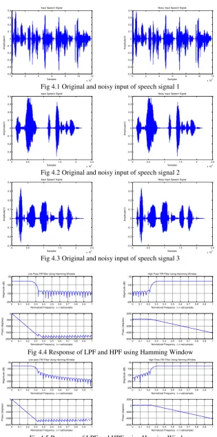
Fig 4.1 Original and noisy input of speech signal 1
Fig 4.2 Original and noisy input of speech signal 2
Fig 4.3 Original and noisy input of speech signal 3
Fig 4.4 Response of LPF and HPF using Hamming Window
Fig 4.5 Response of LPF and HPF using Hanning Window
0 2 4 6 8 10 12
x 104
-0.5 -0.4 -0.3 -0.2 -0.1 0 0.1 0.2 0.3 0.4
Input Speech Signal
Samples
A
m
p
lit
u
d
e
(V
)
0 2 4 6 8 10 12
x 104
-0.5 -0.4 -0.3 -0.2 -0.1 0 0.1 0.2 0.3 0.4
Noisy Input Speech Signal
Samples
A
m
p
lit
u
d
e
(V
)
0 0.5 1 1.5 2 2.5
x 104
-0.4 -0.3 -0.2 -0.1 0 0.1 0.2 0.3 0.4
Input Speech Signal
Samples
A
m
p
lit
u
d
e
(V
)
0 0.5 1 1.5 2 2.5
x 104
-0.4 -0.3 -0.2 -0.1 0 0.1 0.2 0.3 0.4
Noisy Input Speech Signal
Samples
A
m
p
lit
u
d
e
(V
)
0 0.5 1 1.5 2 2.5
x 104
-0.3 -0.2 -0.1 0 0.1 0.2 0.3 0.4
Input Speech Signal
Samples
A
m
p
lit
u
d
e
(V
)
0 0.5 1 1.5 2 2.5
x 104
-0.3 -0.2 -0.1 0 0.1 0.2 0.3 0.4
Noisy Input Speech Signal
Samples
A
m
p
lit
u
d
e
(V
)
0 0.1 0.2 0.3 0.4 0.5 0.6 0.7 0.8 0.9 1
-2000 -1500 -1000 -500 0
Normalized Frequency ( rad/sample)
P
h
a
s
e
(
d
e
g
re
e
s
)
0 0.1 0.2 0.3 0.4 0.5 0.6 0.7 0.8 0.9 1
-200 -150 -100 -50
Normalized Frequency ( rad/sample)
M
a
g
n
it
u
d
e
(
d
B
)
Low Pass FIR filter Using Hamming Window
0 0.1 0.2 0.3 0.4 0.5 0.6 0.7 0.8 0.9 1
-6000 -4000 -2000 0 2000
Normalized Frequency ( rad/sample)
P
h
a
s
e
(
d
e
g
re
e
s
)
0 0.1 0.2 0.3 0.4 0.5 0.6 0.7 0.8 0.9 1
-200 -150 -100 -50
Normalized Frequency ( rad/sample)
M
a
g
n
it
u
d
e
(
d
B
)
High Pass FIR Filter Using Hamming Window
0 0.1 0.2 0.3 0.4 0.5 0.6 0.7 0.8 0.9 1
-2000 -1500 -1000 -500 0
Normalized Frequency ( rad/sample)
P
h
a
s
e
(
d
e
g
re
e
s
)
0 0.1 0.2 0.3 0.4 0.5 0.6 0.7 0.8 0.9 1
-250 -200 -150 -100 -50
Normalized Frequency ( rad/sample)
M
a
g
n
it
u
d
e
(
d
B
)
Low pass FIR Filter Using Hanning Window
0 0.1 0.2 0.3 0.4 0.5 0.6 0.7 0.8 0.9 1
-6000 -4000 -2000 0 2000
Normalized Frequency ( rad/sample)
P
h
a
s
e
(
d
e
g
re
e
s
)
0 0.1 0.2 0.3 0.4 0.5 0.6 0.7 0.8 0.9 1
-250 -200 -150 -100 -50
Normalized Frequency ( rad/sample)
M
a
g
n
it
u
d
e
(
d
B
)
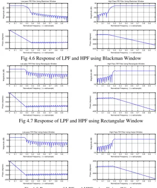
Fig 4.6 Response of LPF and HPF using Blackman Window
Fig 4.7 Response of LPF and HPF using Rectangular Window
Fig 4.8 Response of LPF and HPF using Kaiser Window Fig 4.1, 4.2, 4.3 shows the original and noisy input signal
representation of three speech signals which was spoken by a man. The voice is recorded and it is stored as a wave file for further usage in MATLAB.
Fig 4.4, 4.5, 4.6, 4.7 and 4.8 shows the magnitude and phase response of low pass and high pass filters using Hamming, Hanning, Blackman, Rectangular and Kaiser
windows. The peak amplitude of side lobe for Hamming, Hanning, Blackman, Rectangular and Kaiser windows are -135dB, -125dB, -155dB, -100dB and -100dB respectively.
Fig 4.9 Band 1, 2, 3 and 4 outputs of Hamming window for speech signal1
Fig 4.10 Band 1, 2, 3 and 4 outputs of Hanning window for speech signal1
0 0.1 0.2 0.3 0.4 0.5 0.6 0.7 0.8 0.9 1
-3000 -2000 -1000 0
Normalized Frequency ( rad/sample)
P h a s e ( d e g re e s )
0 0.1 0.2 0.3 0.4 0.5 0.6 0.7 0.8 0.9 1
-250 -200 -150 -100 -50
Normalized Frequency ( rad/sample)
M a g n it u d e ( d B )
Low pass FIR Filter Using Blackman Window
0 0.1 0.2 0.3 0.4 0.5 0.6 0.7 0.8 0.9 1
-6000 -4000 -2000 0 2000
Normalized Frequency ( rad/sample)
P h a s e ( d e g re e s )
0 0.1 0.2 0.3 0.4 0.5 0.6 0.7 0.8 0.9 1
-250 -200 -150 -100 -50
Normalized Frequency ( rad/sample)
M a g n it u d e ( d B )
High Pass FIR Filter Using Blackman Window
0 0.1 0.2 0.3 0.4 0.5 0.6 0.7 0.8 0.9 1
-2000 -1500 -1000 -500 0
Normalized Frequency ( rad/sample)
P h a s e ( d e g re e s )
0 0.1 0.2 0.3 0.4 0.5 0.6 0.7 0.8 0.9 1
-200 -150 -100 -50
Normalized Frequency ( rad/sample)
M a g n it u d e ( d B )
Low pass FIR Filter Using Rectangular Window
0 0.1 0.2 0.3 0.4 0.5 0.6 0.7 0.8 0.9 1
-4000 -2000 0 2000
Normalized Frequency ( rad/sample)
P h a s e ( d e g re e s )
0 0.1 0.2 0.3 0.4 0.5 0.6 0.7 0.8 0.9 1
-150 -100 -50
Normalized Frequency ( rad/sample)
M a g n it u d e ( d B )
High Pass FIR Filter Using Rectangular Window
0 0.1 0.2 0.3 0.4 0.5 0.6 0.7 0.8 0.9 1
-2000 -1500 -1000 -500 0
Normalized Frequency ( rad/sample)
P h a s e ( d e g re e s )
0 0.1 0.2 0.3 0.4 0.5 0.6 0.7 0.8 0.9 1
-200 -150 -100 -50
Normalized Frequency ( rad/sample)
M a g n it u d e ( d B )
Low pass FIR Filter Using Kaiser Window
0 0.1 0.2 0.3 0.4 0.5 0.6 0.7 0.8 0.9 1
-4000 -2000 0 2000
Normalized Frequency ( rad/sample)
P h a s e ( d e g re e s )
0 0.1 0.2 0.3 0.4 0.5 0.6 0.7 0.8 0.9 1
-150 -100 -50
Normalized Frequency ( rad/sample)
M a g n it u d e ( d B )
High Pass FIR Filter Using Kaiser Window
0 5000 10000 15000 -0.4 -0.3 -0.2 -0.1 0 0.1 0.2 0.3
Band1 output of LPF using Hamming window
Samples A m p lit u d e (V )
0 5000 10000 15000 -0.25 -0.2 -0.15 -0.1 -0.05 0 0.05 0.1 0.15 0.2 0.25
Band2 output of HPF using Hamming window
Samples A m p lit u d e (V )
0 0.5 1 1.5 2 2.5 3 x 10⁴ -0.4 -0.3 -0.2 -0.1 0 0.1 0.2 0.3
Band3 output of HPF using Hamming window
Samples A m p lit u d e (V )
0 1 2 3 4 5 6 x 10⁴ -0.2 -0.15 -0.1 -0.05 0 0.05 0.1 0.15 0.2
Band4 output of HPF using Hamming window
Samples A m p lit u d e (V )
0 5000 10000 15000 -0.4 -0.3 -0.2 -0.1 0 0.1 0.2
0.3 Band1 output of LPF using Hanning window
Samples A m p lit u d e (V )
0 5000 10000 15000 -0.25 -0.2 -0.15 -0.1 -0.05 0 0.05 0.1 0.15 0.2
0.25 Band2 output of HPF using Hanning window
Samples A m p lit u d e (V )
0 0.5 1 1.5 2 2.5 3 x 10⁴ -0.4 -0.3 -0.2 -0.1 0 0.1 0.2
0.3 Band3 output of HPF using Hanning window
Samples A m p lit u d e (V )
0 1 2 3 4 5 6 x 10⁴ -0.2 -0.15 -0.1 -0.05 0 0.05 0.1 0.15
0.2 Band4 output of HPF using Hanning window
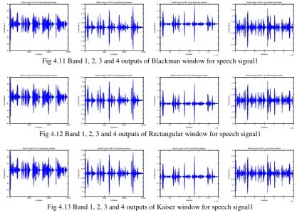
Fig 4.11 Band 1, 2, 3 and 4 outputs of Blackman window for speech signal1
Fig 4.12 Band 1, 2, 3 and 4 outputs of Rectangular window for speech signal1
Fig 4.13 Band 1, 2, 3 and 4 outputs of Kaiser window for speech signal1 From the Fig 4.9, 4.10, 4.11, 4.12 and 4.13 it is observed
that most of the information is present in the band 1. The band 2 contains little less information and also band 2 signals slightly deviates from the original signal. In band 3 the amount of information that is present is very less and
also the information is scattered. In band 4 most of the signal that is present is noise and amplitude levels of this band are also less. Since most of the information is present in the lower frequency band 1, this band almost resembles the original signal.
Fig 4.14 Band 1, 2, 3 and 4 outputs of Hamming window for speech signal2
Fig 4.15 Band 1, 2, 3 and 4 outputs of Hanning window for speech signal2
Fig 4.16 Band 1, 2, 3 and 4 outputs of Blackman window for speech signal2 0 5000 10000 15000
-0.4 -0.3 -0.2 -0.1 0 0.1 0.2
0.3 Band1 output of LPF using Blackman window
Samples A m p lit ud e (V )
0 5000 10000 15000 -0.25 -0.2 -0.15 -0.1 -0.05 0 0.05 0.1 0.15 0.2
0.25 Band2 output of HPF using Blackman window
Samples A m p lit ud e (V )
0 0.5 1 1.5 2 2.5 3 x 10⁴ -0.4 -0.3 -0.2 -0.1 0 0.1 0.2
0.3 Band3 output of HPF using Blackman window
Samples A m p lit ud e (V )
0 1 2 3 4 5 6 x 10⁴ -0.2 -0.15 -0.1 -0.05 0 0.05 0.1 0.15
0.2 Band4 output of HPF using Blackman window
Samples A m p lit ud e (V )
0 5000 10000 15000 -0.4 -0.3 -0.2 -0.1 0 0.1 0.2 0.3
Band1 output of LPF using Rectangular window
Samples A m p lit u d e (V )
0 5000 10000 15000 -0.25 -0.2 -0.15 -0.1 -0.05 0 0.05 0.1 0.15 0.2 0.25
Band2 output of HPF using Rectangular window
Samples A m p lit u d e (V )
0 0.5 1 1.5 2 2.5 3 x 10⁴ -0.3 -0.2 -0.1 0 0.1 0.2 0.3 0.4
Band3 output of HPF using Rectangular window
Samples A m p lit u d e (V )
0 1 2 3 4 5 6 x 10⁴ -0.2 -0.15 -0.1 -0.05 0 0.05 0.1 0.15 0.2
Band4 output of HPF using Rectangular window
Samples A m p lit u d e (V )
0 5000 10000 15000 -0.4 -0.3 -0.2 -0.1 0 0.1 0.2
0.3 Band1 output of LPF using Kaiser window
Samples A m p lit u d e (V )
0 5000 10000 15000 -0.25 -0.2 -0.15 -0.1 -0.05 0 0.05 0.1 0.15 0.2
0.25 Band2 output of HPF using Kaiser window
Samples A m p lit u d e (V )
0 0.5 1 1.5 2 2.5 3 x 10⁴ -0.3 -0.2 -0.1 0 0.1 0.2 0.3
0.4 Band3 output of HPF using Kaiser window
Samples A m p lit u d e (V )
0 1 2 3 4 5 6 x 10⁴ -0.2 -0.15 -0.1 -0.05 0 0.05 0.1 0.15
0.2 Band4 output of HPF using Kaiser window
Samples A m p lit u d e (V )
0 500 1000 1500 2000 2500 3000 -0.015 -0.01 -0.005 0 0.005 0.01
0.015 Band1 output of LPF using Hamming window
Samples A m p lit u d e (V )
0 500 1000 1500 2000 2500 3000 -0.2 -0.15 -0.1 -0.05 0 0.05 0.1
0.15 Band2 output of HPF using Hamming window
Samples A m p lit u d e (V )
0 1000 2000 3000 4000 5000 6000 -0.2 -0.15 -0.1 -0.05 0 0.05 0.1 0.15 0.2
0.25 Band3 output of HPF using Hamming window
Samples A m p lit u d e (V )
0 2000 4000 6000 8000 10000 12000 -0.25 -0.2 -0.15 -0.1 -0.05 0 0.05 0.1 0.15
0.2 Band4 output of HPF using Hamming window
Samples A m p lit u d e (V )
0 500 1000 1500 2000 2500 3000 -0.015 -0.01 -0.005 0 0.005 0.01
0.015 Band1 output of LPF using Hanning window
Samples A m p lit u d e (V )
0 500 1000 1500 2000 2500 3000 -0.2 -0.15 -0.1 -0.05 0 0.05 0.1
0.15 Band2 output of HPF using Hanning window
Samples A m p lit u d e (V )
0 1000 2000 3000 4000 5000 6000 -0.2 -0.15 -0.1 -0.05 0 0.05 0.1 0.15 0.2
0.25 Band3 output of HPF using Hanning window
Samples A m p lit u d e (V )
0 2000 4000 6000 8000 10000 12000 -0.25 -0.2 -0.15 -0.1 -0.05 0 0.05 0.1 0.15
0.2 Band4 output of HPF using Hanning window
Samples A m p lit u d e (V )
0 500 1000 1500 2000 2500 3000 -0.015 -0.01 -0.005 0 0.005 0.01
0.015 Band1 output of LPF using Blackman window
Samples A m p lit u d e (V )
0 500 1000 1500 2000 2500 3000 -0.2 -0.15 -0.1 -0.05 0 0.05 0.1
0.15 Band2 output of HPF using Blackman window
Samples A m p lit u d e (V )
0 1000 2000 3000 4000 5000 6000 -0.2 -0.15 -0.1 -0.05 0 0.05 0.1 0.15 0.2
0.25 Band3 output of HPF using Blackman window
Samples A m p lit u d e (V )
0 2000 4000 6000 8000 10000 12000 -0.25 -0.2 -0.15 -0.1 -0.05 0 0.05 0.1 0.15
0.2 Band4 output of HPF using Blackman window
Fig 4.17 Band 1, 2, 3 and 4 outputs of Rectangular window for speech signal2
Fig 4.18 Band 1, 2, 3 and 4 outputs of Kaiser window for speech signal2 From the Fig 4.14, 4.15, 4.16, 4.17 and 4.18 it is observed
that most of the information is present in the band 1. The band 2 contains little less information and also band 2 signals slightly deviates from the original signal. In band 3 the amount of information that is present is very less and
also the information is scattered. In band 4 most of the signal that is present is noise and amplitude levels of this band are also less. Since most of the information is present in the lower frequency band 1, this band almost resembles the original signal.
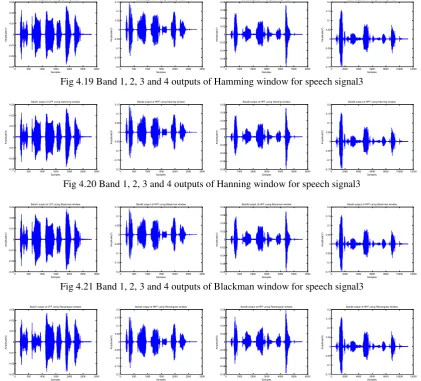
Fig 4.19 Band 1, 2, 3 and 4 outputs of Hamming window for speech signal3
Fig 4.20 Band 1, 2, 3 and 4 outputs of Hanning window for speech signal3
Fig 4.21 Band 1, 2, 3 and 4 outputs of Blackman window for speech signal3
Fig 4.22 Band 1, 2, 3 and 4 outputs of Rectangular window for speech signal3 0 500 1000 1500 2000 2500 3000
-0.02 -0.015 -0.01 -0.005 0 0.005 0.01 0.015
0.02 Band1 output of LPF using Rectangular window
Samples A m p lit ud e (V )
0 500 1000 1500 2000 2500 3000 -0.2 -0.15 -0.1 -0.05 0 0.05 0.1 0.15
0.2 Band2 output of HPF using Rectangular window
Samples A m p lit ud e (V )
0 1000 2000 3000 4000 5000 6000 -0.2 -0.15 -0.1 -0.05 0 0.05 0.1 0.15
0.2 Band3 output of HPF using Rectangular window
Samples A m p lit ud e (V )
0 2000 4000 6000 8000 10000 12000 -0.3 -0.25 -0.2 -0.15 -0.1 -0.05 0 0.05 0.1 0.15
0.2 Band4 output of HPF using Rectangular window
Samples A m p lit ud e (V )
0 500 1000 1500 2000 2500 3000 -0.02 -0.015 -0.01 -0.005 0 0.005 0.01 0.015 0.02
Band1 output of LPF using Kaiser window
Samples A m p lit u d e (V )
0 500 1000 1500 2000 2500 3000 -0.2 -0.15 -0.1 -0.05 0 0.05 0.1 0.15 0.2
Band2 output of HPF using Kaiser window
Samples A m p lit u d e (V )
0 1000 2000 3000 4000 5000 6000 -0.2 -0.15 -0.1 -0.05 0 0.05 0.1 0.15 0.2
Band3 output of HPF using Kaiser window
Samples A m p lit u d e (V )
0 2000 4000 6000 8000 10000 12000 -0.3 -0.25 -0.2 -0.15 -0.1 -0.05 0 0.05 0.1 0.15 0.2
Band4 output of HPF using Kaiser window
Samples A m p lit u d e (V )
0 500 1000 1500 2000 2500 3000 -0.03 -0.02 -0.01 0 0.01 0.02 0.03
Band1 output of LPF using Hamming window
Samples A m p lit ud e (V )
0 500 1000 1500 2000 2500 3000 -0.2 -0.15 -0.1 -0.05 0 0.05 0.1 0.15
Band2 output of HPF using Hamming window
Samples A m p lit ud e (V )
0 1000 2000 3000 4000 5000 6000 -0.08 -0.06 -0.04 -0.02 0 0.02 0.04 0.06 0.08
Band3 output of HPF using Hamming window
Samples A m p lit ud e (V )
0 2000 4000 6000 8000 10000 12000 -0.15 -0.1 -0.05 0 0.05 0.1 0.15 0.2
Band4 output of HPF using Hamming window
Samples A m p lit ud e (V )
0 500 1000 1500 2000 2500 3000 -0.03 -0.02 -0.01 0 0.01 0.02
0.03 Band1 output of LPF using Hamming window
Samples A m p lit u d e (V )
0 500 1000 1500 2000 2500 3000 -0.2 -0.15 -0.1 -0.05 0 0.05 0.1
0.15 Band2 output of HPF using Hanning window
Samples A m p lit u d e (V )
0 1000 2000 3000 4000 5000 6000 -0.08 -0.06 -0.04 -0.02 0 0.02 0.04 0.06
0.08 Band3 output of HPF using Hanning window
Samples A m p lit u d e (V )
0 2000 4000 6000 8000 10000 12000 -0.15 -0.1 -0.05 0 0.05 0.1 0.15
0.2 Band4 output of HPF using Hanning window
Samples A m p lit u d e (V )
0 500 1000 1500 2000 2500 3000 -0.03 -0.02 -0.01 0 0.01 0.02
0.03 Band1 output of LPF using Blackman window
Samples A m p lit u d e (V )
0 500 1000 1500 2000 2500 3000 -0.2 -0.15 -0.1 -0.05 0 0.05 0.1
0.15 Band2 output of HPF using Blackman window
Samples A m p lit u d e (V )
0 1000 2000 3000 4000 5000 6000 -0.08 -0.06 -0.04 -0.02 0 0.02 0.04 0.06
0.08 Band3 output of HPF using Blackman window
Samples A m p lit u d e (V )
0 2000 4000 6000 8000 10000 12000 -0.15 -0.1 -0.05 0 0.05 0.1 0.15
0.2 Band4 output of HPF using Blackman window
Samples A m p lit u d e (V )
0 500 1000 1500 2000 2500 3000 -0.03 -0.02 -0.01 0 0.01 0.02
0.03 Band1 output of LPF using Rectangular window
Samples A m p lit u d e (V )
0 500 1000 1500 2000 2500 3000 -0.2 -0.15 -0.1 -0.05 0 0.05 0.1 0.15
0.2 Band2 output of HPF using Rectangular window
Samples A m p lit u d e (V )
0 1000 2000 3000 4000 5000 6000 -0.08 -0.06 -0.04 -0.02 0 0.02 0.04 0.06
0.08 Band3 output of HPF using Rectangular window
Samples A m p lit u d e (V )
0 2000 4000 6000 8000 10000 12000 -0.15 -0.1 -0.05 0 0.05 0.1 0.15
0.2 Band4 output of HPF using Rectangular window
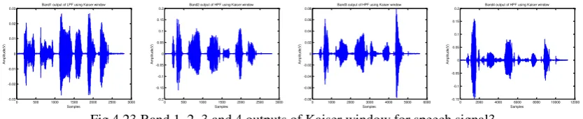
Fig 4.23 Band 1, 2, 3 and 4 outputs of Kaiser window for speech signal3 From the Fig 4.19, 4.20, 4.21, 4.22 and 4.23 it is observed
that most of the information is present in the band 1. The band 2 contains little less information and also band 2 signals slightly deviates from the original signal. In band 3 the amount of information that is present is very less and also the information is scattered. In band 4 most of the signal that is present is noise and amplitude levels of this band are also less. Since most of the information is present in the lower frequency band 1, this band almost resembles
the original signal. The performances of the different windows are evaluated by measuring the leakage factor, main lobe width, side lobe attenuation, peak amplitude of side lobe and Signal to Noise Ratio. Here the performance of Hamming, Hanning, Blackman, Rectangular and Kaiser windows are compared for both the low pass and high pass FIR filters.
Table 4.1 Comparison of leakage factor for different windowing methods
Windowing Methods
Leakage Factor (%)
LPF HPF
Hamming 99.26 100
Hanning 85.11 100
Blackman 84.91 100
Rectangular 99.3 100
Kaiser 99.3 100
Table 4.2 Comparison of main lobe width for different windowing methods
Windowing Methods
Main Lobe Width (-3dB)
LPF HPF
Hamming 0.51953 1.9961
Hanning 0.51953 1.9961
Blackman 0.51172 1.9961
Rectangular 0.53516 1.9961
Kaiser 0.53516 1.9961
Table 4.1 and 4.2 shows the comparison of leakage factor and main lobe width for different windowing methods such as Hamming, Hanning, Blackman, Rectangular and
Kaiser. From the comparison it is observed that Blackman window has minimum leakage factor and smaller main lobe width when compared to other windowing methods. .Table 4.3 Comparison of side lobe attenuation for different windowing methods
Windowing Methods
Side Lobe Attenuation (dB)
LPF HPF
Hamming 0 61
Hanning 0.1 105.3
Blackman 0 116.7
Rectangular 0.8 39.9
Kaiser 0.7 40.5
Table 4.4 Comparison of peak amplitude of side lobe for different windowing methods
Windowing Methods
Peak Amplitude of Side Lobe (dB)
LPF HPF
Hamming -135 -135
Hanning -125 -125
Blackman -155 -155
Rectangular -100 -100
Kaiser -100 -100
0 500 1000 1500 2000 2500 3000 -0.03
-0.02 -0.01 0 0.01 0.02
0.03 Band1 output of LPF using Kaiser window
Samples
A
m
p
lit
ud
e
(V
)
0 500 1000 1500 2000 2500 3000 -0.2
-0.15 -0.1 -0.05 0 0.05 0.1 0.15
0.2 Band2 output of HPF using Kaiser window
Samples
A
m
p
lit
ud
e
(V
)
0 1000 2000 3000 4000 5000 6000 -0.08
-0.06 -0.04 -0.02 0 0.02 0.04 0.06
0.08 Band3 output of HPF using Kaiser window
Samples
A
m
p
lit
ud
e
(V
)
0 2000 4000 6000 8000 10000 12000 -0.15
-0.1 -0.05 0 0.05 0.1 0.15
0.2 Band4 output of HPF using Kaiser window
Samples
A
m
p
lit
ud
e
(V
Table 4.3 and 4.4 shows the comparison of side lobe attenuation and peak amplitude of side lobe for different windowing methods such as Hamming, Hanning, Blackman, Rectangular and Kaiser. From the comparison
it is observed that Hamming and Blackman window have minimum side lobe attenuation for the LPF and Blackman window has minimum peak amplitude of side lobe for both the LPF and HPF.
Table 4.5 Comparison of signal to noise ratio of different windowing methods for speech signal 1
Windowing Methods
Signal to Noise Ratio (dB)
Band 1 Band 2 Band 3 Band 4
Hamming 12.0196 15.4032 14.2775 14.6716
Hanning 12.0638 15.4452 14.3096 14.6662
Blackman 12.1626 15.6137 14.4682 14.6829
Rectangular 11.4783 14.8236 13.8619 14.7123
Kaiser 11.5023 14.8469 13.8782 14.7092
Table 4.6 Comparison of Signal to Noise Ratio of different windowing methods for speech signal 2 Windowing
Methods
Signal to Noise Ratio (dB)
Band 1 Band 2 Band 3 Band 4
Hamming 30.8282 14.7157 11.7933 7.7887
Hanning 30.8056 14.7780 11.8018 7.8552
Blackman 30.8222 15.0322 11.8498 8.1252
Rectangular 30.4593 13.9377 11.4457 6.9922
Kaiser 30.4993 13.9677 11.4665 7.0208
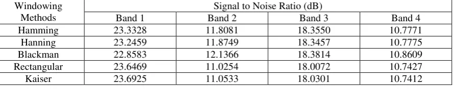
Table 4.7 Comparison of Signal to Noise Ratio of different windowing methods for speech signal 3 Windowing
Methods
Signal to Noise Ratio (dB)
Band 1 Band 2 Band 3 Band 4
Hamming 23.3328 11.8081 18.3550 10.7771
Hanning 23.2459 11.8749 18.3457 10.7775
Blackman 22.8583 12.1366 18.3814 10.8609
Rectangular 23.6469 11.0254 18.0072 10.7427
Kaiser 23.6925 11.0533 18.0301 10.7412
Table 4.5, 4.6 and 4.7 shows the comparison of Signal to Noise Ratio for different windowing methods such as Hamming, Hanning, Blackman, Rectangular and Kaiser. From the comparison it is observed that Blackman window has maximum Signal to Noise Ratio values when compared to other windowing methods.
V. CONCLUSION
In this paper, the bank of finite impulse response filters are used to design the sub-band coding system. Here different windowing methods are used to implement the low pass and high pass finite impulse response filters. Different windowing methods are Hamming, Hanning, Blackman, Rectangular and Kaiser windows. The performance of the different window methods are evaluated based on leakage factor, main lobe width, side lobe attenuation, peak amplitude of side lobe and signal to noise ratio. Finally, the results of different windows are compared and it is observed that Blackman window has minimum leakage factor, side lobe attenuation and peak amplitude of side lobe, smaller main lobe width and provides maximum signal to noise ratio values when compared to other windowing methods.
ACKNOWLEDGEMENT
We thank our PET Engineering College for the motivation and encouragement for giving the opportunity to do this research work as successful one.
REFERENCES
Journal Papers:
[1] Ashraf M. Aziz, Subband Coding of Speech Signals Using Decimation and Interpolation, 13th
International Conference on Aerospace Sciences & Aviation Technology, ASAT- 13, 2009, pp.1-16.
[2] Christian Feldbauer, Marian Kepesi, Klaus Witrisal, Multirate Signal Processing, Signal Processing and Speech Communication Laboratory, V 1.3.3, 2005,pp.1-10.
(IJEEE), Vol. No.6, Issue No. 02, 2014,pp.324-328.
[4] Jagriti Saini and Rajesh Mehra, Power Spectral Density Analysis of Speech Signal using Window Techniques, International Journal of Computer Applications, Volume 131 – No.14, 2015,
pp.33-36.
[5] John G. Proakis and Dimitris G. Manolakis, Digital Signal Processing: Principles, Algorithms and Applications, Third Edition.
[6] Komal Jindal, Analysis of Speech Signals,
International Journal of Computer Science and Mobile Computing (IJCSMC), Vol.3, Issue 3, 2014, pp.795-800.
[7] Lalima Singh, Speech Signal Analysis using FFT and LPC, International Journal of Advanced Research in Computer Engineering & Technology (IJARCET), Volume 4, Issue 4, 2015, pp.1658-1660.
[8] Lalitha R Naik, Devaraja Naik R L, Sub-band Coding Of Noisy Speech Signals Using Digital Signal Processing, International Journal of Advanced Research in Electronics and
Communication Engineering (IJARECE),
Volume 4, Issue 4, 2015,pp.901-904.
[9] Lalitha R Naik, Devaraja Naik R L, Sub-band Coding of Speech Signals using Multirate Signal Processing and comparing the various parameter of different speech signals by corrupting the same speech signal, International Journal of Emerging Trends & Technology in Computer Science (IJETTCS), Volume 4, Issue 2, 2015,pp.217-221. [10]Ljiljana D. Milic, Tapio Saramaki and Robert
Bregovic, Multirate Filters: An Overiew, Proc. IEEE Asia Pacific Conf. on Circuits, Syst., 2006, pp.914-917.
[11]Maurya A.K. and Dr.Deepak Nagarai, Multirate Signal Processing: Graphical Representation & Comparison of Decimation and Interpolation Identities using MATLAB, International Journal of Electronics and Communication Engineering,
Volume 4, 2011, pp.443-452.
[12]Mohammed Mynuddin, Md. Tanjimuddin, Md. Masud Rana, Abdullah, Designing a Low- Pass Fir Digital Filter by Using Hamming Window and Blackman Window Technique, Science Journal of Circuits, Systems and Signal Processing , Vol. 4, No. 2, 2015, pp.9-13. [13]Prajoy Podder, Tanvir Zaman Khan, Mamdudul
Haque Khan and M.Muktadir Rahman,
Comparative Performance Analysis of Hamming, Hanning and Blackman Window, International Journal of Computer Applications, Volume 96–
No.18, 2014,pp.1-7.
[14]Ramya.M, Sathyamoorthy.M, Speech Coding by using Sub band Coding, International Conference on Computing and Control Engineering (ICCCE), 2012.
[15]Raymond N.J. Veldhuis, Marcel Breeuwer, Robbert van der Waal, Subband Coding of Digital Audio Signals Without Loss of Quality,
Philips Research Laboratories, IEEE., vol. A1a.8, 1989, pp. 2009-2012.
[16]Ronald E. Crochiere and Lawrence R. Rabiner, Optimum FIR Digital Filter Implementations for Decimation, Interpolation and Narrow-Band Filtering, IEEE Transactions on Acoustics, Speech, And Signal Processing, Vol. Assp-23, No.5, 1975,pp.444-455.
[17]Saurabh Singh Rajput, Dr.S.S. Bhadauria, Implementation of FIR Filter using Adjustable Window Function and Its Application in Speech Signal Processing International Journal of Advances in Electrical and Electronics Engineering, Volume1, Issue 2, pp.158-164. [18]Saurabh Singh Rajput, S.S. Bhadauria,
Implementation of FIR Filter using Efficient Window Function and Its Application In Filtering a Speech Signal, International Journal of Electrical, Electronic and Mechanical Controls, Volume 1, Issue 1, 2012.
[19]Shikha Shukla, Kamal Prakash Pandev, Rakesh Kumar Singh, Implementation and Simulation of Low Pass Finite Impulse Response Filter Using Different Window Method, International Journal of Emerging Technology and Advanced Engineering, Volume 5, Issue 1, 2015,pp.88-93. [20]Suraj R. Gaikwad and Gopal S. Gawande,
Implementation of Efficient Multirate Filter Structure for Decimation, International Journal of Current Engineering and Technology, Vol.4, No.2, 2014, pp.1008-1010.
[21]Suraj R. Gaikwad, Prof. Gopal Gawande, Review: Design of Highly Efficient Multirate Digital Filters, International Journal of Engineering Research and Applications, Vol. 3, Issue 6, 2013,pp.560-564.
Emerging Trends in Engineering Research (IJETER), Vol. 3 No.6, 2015,pp.257-263.
[23]Suverna Sengar and Partha Pratim Bhattacharya , Multirate Filtering for Digital Signal Processing and its Applications, ARPN Journal of Science and Technology, VOL. 2, NO.3, 2012, pp.228-237.
[24]Vijayakumar Majjagi, Sub Band Coding of Speech Signal by using Multi-Rate Signal Processing, International Journal of Engineering Research & Technology (IJERT), Vol. 2 Issue 9, 2013, pp.45-49.
[25]Vishv Mohan , Analysis And Synthesis of Speech Using Matlab, International Journal of Advancements in Research & Technology, Volume 2, Issue 5, 2013,pp.373-382.
TEXT BOOKS REFERRED
[27]. Sanjit K. Mitra, Digital Signal Processing – A Computer Based Approach, Tata Mc Graw Hill, 2007.
[28]. Andreas Antoniou, Digital Signal Processing,
Tata Mc Graw Hill, 2006.
AUTHOR DETAILS
Dr. P. Kannan (Pauliah Nadar
Kannan) received the B.E. degree from
Manonmaniam Sundarnar University, Tirunelveli, India, in 2000, the M.E. degree from the Anna University, Chennai, India, in 2007, and the Ph.D degree from the Anna University Chennai, Tamil Nadu, India, in 2015. He has been Professor with the Department of Electronics and Communication Engineering, PET Engineering College Vallioor, Tirunelveli District, Tamil Nadu, India. His current research interests include computer vision, biometrics, and very large scale
integration architectures.
.
G.Bharatha Sreeja received B.E