A Marketing-Oriented Inventory Model with Three-Component Demand Rate and Time-Dependent Partial Backlogging

(1)

https://dx.doi.org/10.24001/ijaems.3.3.11 ISSN: 2454-1311

A Marketing-Oriented Inventory Model with

Three-Component Demand Rate and

Time-Dependent Partial Backlogging

Dr. Samiran Senapati

Department of Mathematics, Nabadwip Vidyasagar College, Nabadwip, West Bengal, India.

Abstract— This paper, an attempt has been made to extend the model of “An EOQ model for perishable items under stock-dependent selling rate and time-dependent

partial backlogging” with a view to making the model

more flexible, realistic and applicable in practice. Here, objectives are to maximize the profit and minimize the total shortage cost. In this model, fuzzy goals are used by linear membership functions and after fuzzification, it is solved by weighted fuzzy non-linear programming technique. The model is illustrated with a numerical

example adopted partially from “An EOQ model for perishable items under stock-dependent selling rate and time-dependent partial backlogging”.

Keywords— EOQ; Perishable items; Partial back logging; Fuzzification; Membership function.

I. INTRODUCTION

In the competitive market situation, it is commonly observed that an increase in shelf space and glamorous display for an item induce more consumers to buy it. Recently, Dye and Ouyang (2005) investigated an economic order quantity (EOQ) model for perishable items under stock-dependent selling rate and time-dependent partial backlogging. In two-component demand, it is assumed that the demand rate is stock-dependent down to a certain level and then it becomes constant. But, it is commonly observed that the demand rate will not be dependent on displayed stock level for a huge amount of stock as all available stock cannot be displayed properly and glamorously because of cost of modern light, electronic arrangement and space will be increased ( e.g. fashionable goods shop). It will be dependent on displayed stock level within a range and beyond this range, it will be quite uniform. This type of demand rate is called three-component demand rate.

It has been recognized that one’s ability to make precise

statement concerning an inventory model diminishes with increasing complexities of the system. Generally, it may not be possible to define the objective goals precisely. In reality, management is most likely to be uncertain of the true value of parameters and due to many unforeseen

incidents like strike, hike in wages, increased transportation cost etc; hence during the course of business, a vendor or decision maker is forced to settle down with a lower profit amount compared to the profit as he/she normally has targeted due to adverse situation. Moreover, shortages bring loss of goodwill for the vendor. This loss can not be measured numerically. For this reason, it is advisable to restrict the shortages as much as possible to minimize the loss of goodwill. From the above discussion, we may conclude that it is difficult to determine the exact amount of profit and shortage cost rather a range may be fixed for these. Hence, under these phenomena the inventory model may be better treated in a fuzzy system.

II. NOTATIONS AND MODELING ASSUMPTIONS

In this section, we give the notations and assumptions used throughout this chapter.

2.1 The inventory system involves only one item. 2.2 Replenishment rate is infinite and lead time is

zero.

2.3 θ, constant rate of deterioration. I(t) is the inventory level at time t (Fig. 1).

2.4 p, the selling price per unit and A, the ordering cost per order, are constant.

2.5 The unit cost C and the inventory carrying cost as fraction i, per unit per unit time, are constant.

2.6Shortages are allowed and backlogged rate is

defined to be 1/[1+ δ(T-t)]. The backlogging

parameter δ is a positive constant. Shortage

cost is C2 per unit per unit time and R is the fixed opportunity cost of lost sales per unit. 2.7 The demand rate D(p, I(t)), is dependent on

(2)

α (p) + βS1 I(t) ≥ S1,

α (p) + βI(t) S0 ≤ I(t) ≤ S1, D(p, I(t)) = α (p) 0 ≤ I(t) ≤ S0,

_

 

_

t T δ 1 p α 

 I(t) ≤ 0

Where, β is a non-negative constant. α (p) is a non -negative function of selling price p.

2.8 Shortages are allowed and backlogged rate is

defined to be 1/[1+ δ(T-t)]. The backlogging

parameter δ is a positive constant. Shortage cost is C2 per unit per unit time and R is the fixed opportunity cost of lost sales per unit. 2.9 T is the cycle time.

2.10TP and SC respectively denote the total

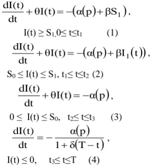
III. THE MATHEMATICAL MODEL At the beginning of the order cycle the inventory level is raised to Q afterwards as time progresses it is depleted by combined effects of the demand and deterioration. The pictorial representation of the inventory system is given in Fig. 1. Therefore, the differential equations governing the system during the period (0 ≤ t ≤ T) can be written as:

θI(t)



α

 

p βS₁



dt

dI(t)_ __ _ ,

I(t) ≥ S1,0≤ t≤t1 (1)

 



αp βI t



θI(t) dt dI(t) 1     ,

S0 ≤ I(t) ≤ S1, t1≤ t≤t2 (2)

 

p α θI(t) dt

dI(t)

  ,

0 ≤ I(t) ≤ S0, t2≤ t≤t3 (3)

 



T t



δ 1 p α dt dI(t)     ,

I(t) ≤ 0, t3≤ t≤T (4)

The solutions of the above differential equations, after applying boundary conditions I(t1) = S0, I(t2) = S1, I(t3) = 0, are

 





























          

1 t

θ

e

θ

1 βS

p

α

t

1 t

θ

e

1 S

I(t)

0≤ t ≤ t1 (5)

  

 







e   1



β θ p α e S

I(t) ₀ θ β t2 t θ β t2 t 

 

     _,

t1≤ t ≤ t2 (6) (6)

 



_e   ₁



θ p α

I(t) θt3 t  _,

t2≤ t≤t3 (7)

 

_

_

_

_

_

_

t T δ 1 ln t T δ 1 ln δ p α

I(t)    ₃   

t3≤ t≤T (8)

Ordering cost per cycle = A Holding cost per cycle =

 

         

_



3 2 2 1 1 t t t t t 0 dt t I dt t I dt t I Ci

Shortage cost per cycle (SC) =

 

_

_

_

_

_

_



     T t 3 2 3 dt t T δ 1 ln t T δ 1 ln δ p α C

Opportunity cost due to lost sales per cycle =

 

_

_

_

         T t3 dt t T δ 1 1 1 R p α Purchase cost

 

_

_



 



_

_

           

 e 1

θ βS p α e S t T δ 1 ln δ p α

C θt1 1 θt1

1 3

Sales revenue per cycle =

 







 



       

_



2 1 1 t t t 0

1 dt αp βI t dt βS p α S

 





_

 

_

       

_



T t 3 t t 1 3 3 2 dt t T δ 1 p α dt βS p α

on integration and simplification of the relevant costs mentioned above, the total profit per unit time TP becomes, TP=

   





  



    _ _ _ _ Rδ C δ p α t T δ 1 ln C -p δ p α 2 2 3











δT-t3 -ln1δTt3





_





  _



_

  

1 e

Ci

βS θ β t2 t1

 











 

3 1 1



θt 1 2 0 t βS t p α p 1 e θ CiS β θ p α β θ S

1  

           

 



 _

_

_

_

_



_



 





_

  ₂ 1

2 3 t t θ 2 _θ βS p α Ci 1 t t θ e θ p α

Ci 3 1



eθt1θt₁1



 





_θ _β

 

t1 t2



Ci pβ p α A     

 

_

_

T 1 e θ βS p α e S

C 1 θt1 1 θt 

         _ 

 , (9)

and total shortage cost per unit time,

 

_

_

_

_

_

_

T dt t T δ 1 ln t T δ 1 ln δ p α C SC T t 3 2 3



      (10)

where S0 and S1 is given by,

 







 



θ βt2 t1

0 1 e β θ p α S β θ p α

S _  

         

 , (11)

   

θt3 t2

0 e θ p α θ p α

S    , (12)

(3)





 





 







 

 

   

 

 

  

β θ

p α S

β θ

p α S ln β θ

1 t t

0 1 1

2 , (13)

 

   

 

   



 _

 

θ p α

θ p α S ln 1 t t

0 2

3 _ , (14)

The above two equations implies

t2 – t1> 0, (15) and t3 – t2> 0, (16)

and the initial lot size

 























e

θt

1

1 θ

1 βS

p

α

1 θt

e

1 S

I(0)

Q

,

(17)

Replacing t1by 0 first, substitute t2 and t3 by t1, we can observed that the above profit function will be same as the profit function of Dye and Ouyang (2005).

5.1. Crips model

In crisp environment multi-objective problem of maximizing total profit and minimizing the total shortage cost can be written as follows:

Max TP Min SC

Subject to, t2 – t1> 0 t3 – t2>0

where t1, t2, t3, T ≥ 0. (18)

5.2Fuzzy model

Since seller’s maximum average revenue and minimum

total shortage cost per unit time becomes imprecise in nature, the above model in fuzzy sense can be represented as:

TP

x

~

Ma

SC

n

~

Mi

Subject to, t2 – t1> 0 t3 – t2>0

where t1, t2, t3, T ≥ 0. (19)

5.3 Fuzzy goal programming of model

The fuzzy multi-objective problem can be formulated as a FNLGP as follows:

Find (t1, t2, t3, T)T subject to the constraints f1( t1, t2, t3, T ) = -TP ≤ -f01 f2( t3, T ) = SC ≤ f02 t2 – t1> 0

t3 – t2>0 where t1, t2, t3, T ≥ 0.

Here, the fuzzy goal of objectives, i.e. total average profit and total shortage cost, are (f01-P01, f01) and (f02, f02+P02) respectively, and there linear MFs are consider as follows:

0,for f1(t1, t2, t3, T) ≤ - f01+P01

µ1(f1(t1, t2, t3, T)) =





01

01 3

2 1 1

P

f

T

,

t

,

t

,

t

f

1 



,

for -f01 ≤ f1(t1, t2, t3,T) ≤ -f01+P01 1, for f1(t1, t2, t3, T) ≤ - f01 i.e.

0, for TP ≤ f01- P01

µ1(TP) =

01 01

P

f

-TP

1 

, for f01- P01≤ TP ≤ f01

1,for TP ≥ f01 and

0, for SC ≥ f02 + P02

µ2(SC)=

02 02

P

f

SC

1 



,for f02≤ SC ≤f02 +

P02

1, for SC ≤ f01

Using the weights to represent different importance for the objectives, the problem can be written as follows:

Max F = w1µ1(TP) + w2µ2(SC) Subject to

f01-P01≤ µ1(TP) ≤ f01

f02≤ µ2(SC) ≤ f02+P02 t2 – t1> 0

t3 – t2>0 w1 + w2 = 1 where t1, t2, t3, T ≥ 0.

IV. NUMERICAL EXAMPLES To illustrate the above inventory models, values of the system parameters are considered as:

A = 250.0, β = 0.3, θ = 0.08, C = 5.0, i = 0.35, C2=3.0,

p=7.0, R=5.0, δ = 10,

 

r

K(p)

p

α



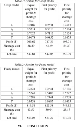
 , K = 20000.0, p=7.0,S0 = 100.0, S1= 300.0, r = 1.5, f01 = -$750.0, f02 = $30.0, P01 = -$625.0, P02 = $20.0.

The optimal values of t1, t2, t3, t4 along with total profit, total shortage cost and lot-size are displayed below: From Table-1 and Table-2, it is observed that when a seller takes care of his profit only, the seller makes maximum revenue at the cost of his reputation and goodwill. Similarly when the seller only takes care of his shortage cost, his total revenue is lower. As expected,

when interests of both seller’s total revenue and shortage

(4)

V. FIGURES AND TABLES

Table.1: Results for Crisp model Crisp model Equal

weight for profit & shortage cost

First priority for profit

First priority

for shortage

cost

t1 0.2489 0.2531 0.2613

t2 0.5214 0.5310 0.5124

t3 0.7025 0.7112 0.7124

T 0.9678 0.9852 0.9675

Profit ($) 709.62 717.39 693.71 Shortage cost

($)

58.29 63.69 54.20

Lot-size 537.81 542.05 550.39

Table.2: Results for Fuzzy model Fuzzy model Equal

weight for profit & shortage cost

First priority for profit

First priority

for shortage

cost

t1 0.2521 0.2641 0.3196

t2 0.5247 0.5482 0.5772

t3 0.7288 0.7441 0.7738

T 0.9558 0.9885 0.9435

Profit ($) 819.51 825.38 744.12 Shortage cost

($)

43.59 50.04 25.17

Lot-size 543.05 533.22 610.36

VI. CONCLUSION

A multi-objective inventory model of deteriorating item with stock and price dependent demand, with shortages is developed. Here a real-life inventory problem faced by the inventory practitioners is considered. The purpose of this chapter is to investigate an inventory model for deteriorating item with three-component demand rate;

permitting shortage and time-proportional backlogging rate within the economic order quantity (EOQ) framework. In the existing model Dye and Ouyang (2005), authors considered the demand rate dependent on the current displayed stock, i.e. the demand rate will be high and high for more and more displayed stock in the showroom. This is somehow unrealistic. The stock dependency nature must occur within a range, and beyond this range it will be quite uniform. Selling price is also an influencing factor on demand. Under fire over various financial ethical issues globally, some attention must be need to the replenishment cost so that it becomes minimum along with the maximum profit. Such a realistic problem has been modeled and solved under crisp and fuzzy environment. Since the proposed model has been formulated with imprecise informations, the decision maker may choose that solution which suits him/her best respect to conditions and restrictions. Till now, only a very few researchers have considered such a realistic phenomenon, though several papers dealing with an EOQ model with deterioration and time-dependent partial backlogging are available.

The scope of application of the model in supermarkets is open however, success depends on correctness of the estimation of input parameters. To estimate the parameters, demands of the same kind product in different supermarkets have to be observed and analyzed over long time.

ACKNOWLEDGEMENTS

I am grateful to express my reverence to my honorable teachers of Department of Mathematics, University of Kalyani. For the source of relevant of information, I am indebted to the librarians of Indian Institute of Management, Kolkata, and Indian Statistical Institute, Kolkata. I am also thankful to the librarians and the others members of staff of the libraries of the department. I convey my heart left thanks to Dr. Shibaji Panda, Bengal Institute of Technology, Kolkata – 700150, Dr. Subrata Saha, Dr. Kanailal Banerjee and all of my friends, Colleagues of Nabadwip Vidyasagar College, Research Scholars and all other well-wishers of Department of Mathematics, University of Kalyani for the co-operation, helps and inspiration during the period of my research work.

I sincerely remember and acknowledge the encouragement of my family members extended to me to complete my research work.

REFERENCES

[1] Abad, P.L. (1988), ‘Determining optimal selling

price and lot size when the supplier offers all-unit

t

1

t

2

t

3

T

0

Time

S

1

S

0

Fig. 1. Graphical representation of inventory system

I

n

v

en

to

ry

lev

(5)

quantity discounts’. Decision Sciences, 19, 622 -634.

[2] Abad, P.L. (1996), ‘Optimal pricing and lot sizing

under condition of perishability and partial

backordering’. Management Science, 42, 53-65. [3] Abad,P.L. (2000),‘Optimal lot-size for a perishable

good under conditions of finite production and

partial backordering and lost sale’. Computers and

Industrial Engineering, 38, 457-465.

[4] Aggarwal, S. P. and Goel, V. P. (1985), ‘Order

level inventory system with power demand pattern

for deteriorating items’. Proceeding of all India

Seminar on Operational Research and Decision Making, University of New Delhi, New Delhi, 19 - 34.

[5] Aggarwal, S. P. and Jaggi, C. K. (1995), ‘Ordering

polices of deteriorating items under permissible

delay in payments’. Journal of Operational Research

Society,46, 658–662.

[6] Anily, S. (1995), ‘Single-machine lot sizing with uniform yields and rigid demands: Robustness of the

optimal solution’. IIE Transactions 27(5), 633-635. [7] Anupindi, R. and Bassok, Y. (1999),‘Centralization

of stocks: Retailers Vs. Manufacturer’. Management

Science, 45, 178–191.

[8] Arani, M. and Rand, G. K. (1990), ‘An electronic

algorithm for inventory replenishment for items with

increasing linear trend in demand’. Engineering,

Costs and Production Economics, 19, 261–266. [9] Arcelus, F. J. and Srinavasan, G. (1995),‘Discount

strategies for one time only sales’. IIE Transactions,

27, 618–624.

[10]Arcelus, F. J. and Srinavasan, G. (1998),‘Ordering policies under one time discount and price sensitive

demand’. IIE Transactions, 30, 1057–1064.

[11]Ardalan, A. (1988), ‘Optimal ordering policies in response to a sale’. IIE Transactions, 20, 292–294. [12]Ardalan, A. (1991), ‘Combined optimal price and

optimal inventory replenishment policies when a

sale results in increase in demand’. Computers and

Operations Research, 18, 721–730.

[13]Arrow, KJ. Harris, T. and Marschak, J. (1951),

‘Optimal inventory policy’. Econometrica, XIX.

[14]Arrow, KJ. Karlin, S. and Scarf, H. (1958), ‘Studies in the Mathematical Theory of Inventory and Production’. Stanford, California, Stanford

University Press.

[15]Baker, RC. and Urban, TL. (1988), ‘A

deterministic inventory system with an inventory

level dependent demand rate’. Journal of the Operational Research Society, 39, 823 - 831. [16]Balkhi, Z. T. (2004), ‘An optimal solution of a

general lot-size inventory model with deteriorated an

imperfect product, taking into account inflation and

time value of money’. International Journal of

System Science, 35(2), 87–96.

[17]Barbosa, L. C. and Friedman, M. (1978),

‘Deterministic inventory lot-size models – A general

root law’. Management Science, 24, 819 – 826. [18]Barron, L. E. C., (2000), ‘Observation on:

Economic production quantity models for items with

imperfect quality’. International Journal of

Production Economics, 641, 59-64.

[19]Basu, M and Banerjee, K. L. (2001),‘An algorithm

for determining EOQ under quantity dependent unit

production cost’. Proceedings of an International

Conference on Operational Research and National Development, 116–118.

[20]Basu, M., Ghosh, D. and Banerjee, KL. (1999),‘A

solution procedure for solving multi-item inventory

problem’. International Journal of Management and

Systems, 15(1), 53 - 68.

[21]Basu, M., Pal, BB. andGhosh, D. (1991), ‘The

priority preferenced goal programming method for solving multi-objective dynamic programming

Models’. Advances in Modeling and Simulation,

22(2), 49 - 64.

[22]Basu, M., Panda, S. and Banerjee, K. L. (2005),

‘Determination of EOQ of multi-item inventory problems through non-linear goal programming with

penalty function’. Asia Pacific Journal of

Operational Research, 22(4), 539-553.

[23]Basu, M., Panda, S., Senapati, S. and Banerjee, K. L. (2005), ‘Determination of EOQ of multi-item inventory problems through non-linear goal

programming’. Advanced Modelling and

Optimization, 7(2), 169–176.

[24]Basu, M., Senapati, S. and Banerjee, K. L. (2006), ‘A multi-item inventory model for deteriorating items under inflation and permissible delay in payments with exponential declining demand’. Opsearch, 43(1), 71-87.

[25]Bellman, R. E. and Zadeh, L. A. (1970),‘Decision

-making in a fuzzy environment’. Management

Science, 17, B141–164.

[26]Ben-daya, M. and Raouf, A. (1993), ‘On the

constrained multi-item single period inventory

problem’. International Journal of Operations and

Production Management, 13, 101-112.

[27]Ben-daya, M. and Raouf, A. (1994), ‘Inventory models involving lead time as decision variable’.

Journal of Operational Research Society, 45, 579– 582.

[28]Ben-Deya, M. and Hariga, M. (2000), ‘Economic

(6)

process’. Journal of the Operational Research

Society, 51, 875- 881.

[29]Bernstein, F. and Federgruen, A. (2004),‘Dynamic

inventory and pricing models for competing

retailers’. Naval Research Logistics, 51, 248 – 274. [30]Beyer, D. (1994),‘An inventory model with Weiner

demand process and positive lead time’.

Optimization, 29, 181–193.

[31]Biermans, H. and Thomas, J. (1977), ‘Inventory

decisions under inflationary conditions’. Decision Sciences, 8, 151–155.

[32]Billington, P. J. (1977),‘The classic economic

production quantity model with set-up cost as a

function of capital expenditure’. Decision Sciences,

18, 25–42.

[33]Bose, S., Goswami, A. and Chaudhuri, K. S. (1995),‘An EOQ model for deteriorating items with

linear time-dependent demand rate and shortages

under inflation and time discounting’. Journal of

Operational Research Society, 46, 771 – 782. [34]Brahmbhatt, A. C. (1982),‘Economic order quantity

under variable rate of inflation and mark-up prices’. Productivity, 23, 127–130.

[35]Buchan, J. and Koenigsberg, E. (1963),‘Scientific Inventory Management’. Prentice Hall, Englewood

Cliffs, NJ.

[36]Burewell, T. H., Dave, D. S., Fitzpatrick, K. E. and Roy, M. R. (1991),‘An inventory model with planned shortages and price dependent demand’.

Decisions Sciences, 27, 1181–1191.

[37]Buzacott, J. A. (1975), ‘Economic order quantities with inflation’. Operational Research Quarterly, 26,

553–558.

[38]Cadenas, J. M.; Pelta, D. A., Pelta, H. R. and Verdegay, J. L. (2004), ‘Application of fuzzy optimization to diet problems in Argentinean firms’.

European Journal of Operational Research, 158, 218–228.

[39]Cakanyildirim, M., Bookbinder, J. H. and Gerchak, Y. (2000), ‘Continuous review inventory models where random lead time depends on lot size

and reserved capacity’. International Journal of

Production Economics, 68, 217–228.

[40]Chakraborty, R and Patra, N. K. (2003), ‘A

stochastic inventory model for a finite life item with uniform lead time and demand depending on m

different types of quality’. International Journal of

Management and Systems, 19, 11 – 24.

[41]Chakravarty, A.K. and Shtub, A. (1987), ‘Strategic

allocation of inspection effort in a serial,

multi-product multi-production systems’. IIE Transactions 19(1), 13 – 22.

[42]Chandra, J. M. and Bahner, M. L. (1988), ‘The

effects of inflation and the value of money or some

inventory systems’. International Journal of

Production Research, 23(4), 723 – 730.