Available online at: www.ijcncs.org ISSN 2308-9830
A Mat-Lab based Filter for curtailing Interferences in Ad-Hoc
Network
FAKIR MASHUQUE ALAMGIR1, CHRISTER ANDREWS2, JANNATUL FERDOUS KAKON3
1
Senior Lecturer, 2, 3 Department of Electrical & Electronics Engineering, East West University, Dhaka.
E-mail: [email protected], [email protected], [email protected]
ABSTRACT
A wireless ad-hoc network is a new archetype in wireless communication which doesn’t require any fixed infrastructure such as base stations or mobile switching center. Reducing interference is one of the main challenges in wireless ad hoc networks. The main aim of this thesis is to study various issues pertaining to wireless ad-hoc network and find ways to diminish the interference effect in this network. Starting with basic knowledge of ad-hoc networks, its applicability, security issues, and this thesis digs into details of existing research works in minimization of interference effect in ad-hoc network. Next the thesis work focuses on new ways to diminish the interference effect in ad-hoc network. A new solution is recommended to achieve our main goal which is both cost effective and simple. It is observed that the proposed minimization technique is an effective one.
Keywords: Enfumble average, Ad-hoc, Base station, Interference, Minimization.
1 INTRODUCTION
Wireless networks have received a considerable amount of required interest in the last decade due to the fact that users can connect easily to the network without any wires. ‘An ad-hoc network is a self-organizing multi-hop wireless network, which relies neither on fixed infrastructure nor on predetermined connectivity.’ [2]. It can also be very useful when there is no possibility of setting up fixed networks due to geographical restrictions or cost ineffectiveness. Now major concern in wireless network is interference which ruins the desired communication between two users if any new user appears operating in the same or nearly same frequency.
2 IMPACTS OF INTERFERENCE
Packets of data are regularly sent in between neighboring nodes in ad-hoc network. These packets of data experience interference which is caused by simultaneous communications between other nodes in the network. ‘The interference of a network is defined as the largest number of sensors that can directly communicate with a single plane
in the plane. ‘One of the main challenges in models of wireless communication is interference. For instance, a node A may interfere with another node B if A's interference range unintentionally covers B. Consequently, the amount of interference that B experiences is the number of such nodes A. [3]. The main aim of the interference reduction is to maximize the capacity and throughput of the system. Interference can be reduced by having nodes send with less transmission power. The area covered by the smaller transmission range will contain fewer nodes, yielding less interference. On the other hand, reducing the transmission range has the consequence of communication links being dropped. However, there is surely a limit to how much the transmission power can be decreased. In ad hoc networks, if the node's transmission ranges become too small and too many links are abandoned, the network may become disconnected. Hence, transmission ranges must be assigned to nodes in such a way that the desired global network properties are maintained. [3].
Fig. 1. Arrangement of simulation laptops
The laptops L2 and L3 are connected to the ad-hoc network created by the laptop L1 and the laptops are moved at various distances to analyze the interference effect and the signal strength by using the simulation softwares. The software named VISTUMBLER is used here to analyze the ad-hoc connection between the laptops in the network. The X-axis of the graph shows the signal strength and the Y-axis shows the time.
Fig. 2. VISTUMBLER- shot 1
In shot 1 of VISTUMBLER simulation, it can be observed that initially the signal strength is 100% but as time goes by the signal strength reduces. This degradation in the graph is due to the movement of other laptops in the network to a certain distance from the central laptop, L1 with respect to time.
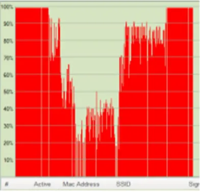
Fig. 3. VISTUMBLER- shot 2
In shot 2, it is seen that the signal strength decreased gradually as the laptops were moved farther apart from each other and the minimum signal strength reached was 20%. The signal strength increased as the laptops were gradually brought closer. A point for lookout is that in the middle of the graph the signal strength suddenly dropped to 20% from 45% for a very short time which was due to the unexpected interference of an external laptop. Then as time passed by, signal strength increased gradually.
In shot 3, it is observed that the signal strength has reached 100% as all the laptops in the network are close to each other.
Now let us observe the simulation results generated by the software INSSIDER to check the interference between the laptops in the ad-hoc network which are as follows:
Fig. 5. INSSIDER- shot 1
Here only single laptop is in the adhoc network. So the signal amplitude is constant at -35 dB. There are no other interference.
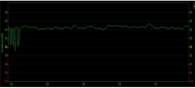
Fig. 6. INSSIDER- shot 2
Here L2 is added to the network created by L1. The signal amplitude decreases as there is interference in between L1 and L2.
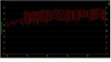
Fig. 7. INSSIDER- shot 3
Next, L3 was kept in front of L1 while the connection between L1 and L3 was established. Now a great change can be seen. The signal strength is more compared to the previous one. This shows the uncertainty of the wireless networks.
Fig. 8. INSSIDER- shot 4
Fig. 9. INSSIDER- shot 5
The two simulation graphs above show the increased interference as the laptops were moved farther apart from L1.
Fig. 10. INSSIDER- shot 6
The interference reached its maximum when an external laptop entered into the network.
The above figure show that the signal almost faded away as the laptops were nearly out of range of L1.
Fig. 12. INSSIDER- shot 8
This is the final scenario when all the connections are disconnected in the network and the amplitude is constant at -35dB.
3 PROPOSED FILTER
Minimization of interference in ad-hoc network is an explanatory research methodology. A design of filter is proposed to reduce the interference effect or it can be said an algorithm is developed which can be useful in the world of ad-hoc networks. This can in turn increase the capacity of network which can be useful in future development. The research focuses on the extending the current theory for the interference handling in ad-hoc networks. The main aim of this thesis is to mitigate the effect of interference in a wireless ad-hoc network. For mitigation, some mathematical equations are used which can further be used for making a filter to tackle the interferers which are none other than users who are not supposed to be in that network. Here one estimated filter model is described to work with simulation results provided from some equations. The interferer can be related to Hidden and Exposed node problem. A simple model is taken to describe a basic receiver. The equation used is as follows:
n
Hx
Y
(1) Here Y is the received signal. It is a (n*1) matrix.
n is the length of the filter.
H is the (n*n) channel matrix
K K K K
h
h
h
h
h
h
h
h
h
h
h
h
H
4 42 41 3 32 31 2 22 21 1 12 11...
...
...
...
(2) X is the transmitted signal of (n*1) matrix sent by k number of users.
N is the Gaussian noise of (n*1) matrix from the channel which cannot be tolerated. It has to be considered with the received signal whenever any assumption is taken. Now the general notion is when a signal is transmitted and received by the receiver, in general, it is not possible to get the actual signal when it is received. So error minimization technique is used. This can be described with an equation which is as follows:
1 1 1
~
x
x
e
(3)
e1 = error in estimation x1 = transmitted signal
1
~
x
estimated signalThe above equation shows the error in estimation can be calculated and can also be minimized so that the receiver can get nearly same signal as the transmitted one. The estimated error should be as less as possible to retrieve the required signal. An LMS approach is used to train the filter coefficient so that after a number of trains, the desired signal can be achieved. It can be said an adaptive LMS algorithm is used to update the linear filter coefficients.
1
~
x
can also be written as:y
T i i
x
g
~
(4)
Here g1 is the actual received signal.
This is the part of the method which is known as Linear MMSE- Wiener solution. Now the new formula used to determine the signal is:
2min
min
y
T i i
x
E
g
(5) min
= mean square error (MSE)Here the information bits used are BPSK (Binary Phase Shift Keying) as the information can only be +1 or -1 which makes the estimation little easy.
%The random spreading-sequence is generated for every simulation
rand('state',sum(100*clock)) SprSeq=randn(Users,SprGain); for k=1:Users
SprSeq(k,:)=SprSeq(k,:)/sqrt(sum(SprSeq(k,:).^2)); end
%The packets change for every simulation. So, does the received
%signal-symbol vector
rand('state',sum(100*clock)) x_bpsk=sign(rand(Users,lx)-0.5); r_ch=zeros(1,lx*SprGain); for n=1:lx
tmp=0; for k=1:Users
tmp=SprSeq(k,1:SprGain)*x_bpsk(k,n)+tmp; end
The mean square error (MSE) formula can also be written as:
min
=
Ltrain
i 0
2
~
ii
x
x
(6)
Here Ltrain is the training length which is taken as 6000 in this project for better understanding of MSE. The lower MSE will mean less error which means a better received signal. The load ratio is defined as the ratio of the number of users by the spreading gain. So load ratio changes for every number of users added and when the load ratio is <1, then the system is said to under saturated. When it comes to >1, then the system is said to be oversaturated. A multiuser detector filter has been employed as a model filter so that it can be entertained to make the simulation more realistic. The coefficients for the forward and backward coefficients of filter area are taken as Successive DFD (S - DFD) and Parallel DFD (P- DFD) respectively.
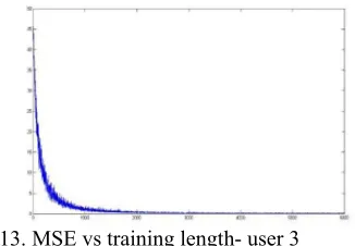
The following figures are MATLAB plots of MSE vs Training length for different number of users. The X-axis shows the number of training length used and Y-axis shows the MSE.
Fig. 13. MSE vs training length- user 3
It can be seen that for a training length between 0-1000 the fluctuation of MSE is greater which represents interference in the network. The fluctuation is expected to increase as the number of user increases.
Fig. 14. MSE vs training length- user 7
Fig. 15. MSE vs training length- user 12
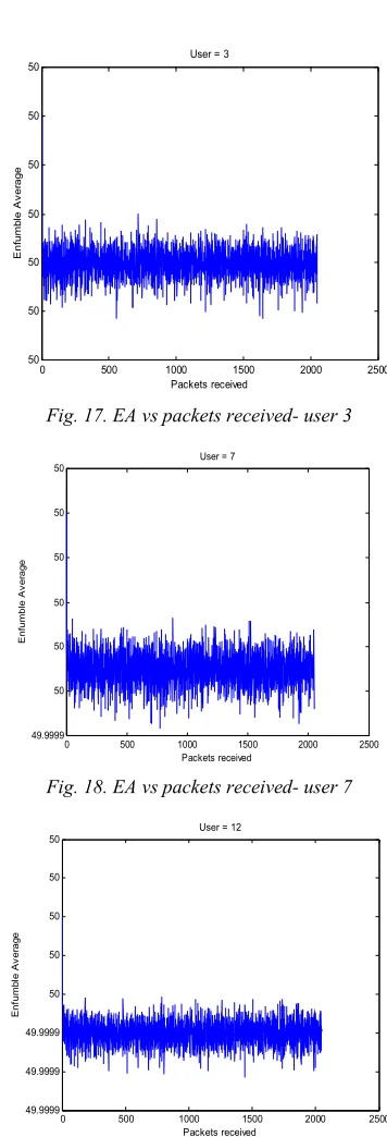
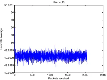
Now an average called Enfumble average (EA) is used to show the average MSE of last 200 packets received by the system. This is done to verify whether the estimated filter works reliably and transmits all the information to the receiver.
MSE fluctuation due to interference between more numbers of users can be described by the following Matlab code:
wf=zeros(Users,FFFsize); wb=zeros(Users,FBFsize); mse_t=zeros(Users,ltrain);
for k=1:Users for n1=1:ltrain z1=0;
for n2=1:FFFsize
z1=z1+wf(k,n2)*r((n1-1)*SprGain+n2); end
for n2=1:FBFsize %Parallel DFD type, all the users-interference is taken onboard
z1=z1-wb(k,n2)*xtrain(n2,n1); end
er1= xtrain(k,n1)-z1; mse_t(k,n1)=er1*er1;
The first two lines show the initial value of forward and backward filter coefficient as wf and wb respectively.
The first for loop is for training length till 6000 loops.
The second for loop is for the forward filter coefficient.
The third for loop is for the backward filter coefficient z1 decreases for a certain extent and then fluctuates as the maximum threshold level is reached for the particular user.
Now we shall see plots of EA vs packets. Here an average called Enfumble average (EA) is used to show the average MSE of last 200 packets received by the system.
The following figures are MATLAB plots of Enfumble average vs packets received for different number of users. The X-axis shows the Enfumble average and Y-axis shows the packets received.
Fig. 17. EA vs packets received- user 3
Fig. 18. EA vs packets received- user 7
Fig. 19. EA vs packets received- user 12
0 500 1000 1500 2000 2500 50
50 50 50 50 50 50
Packets received
E
nfumb
le
A
v
er
ag
e
User = 3
0 500 1000 1500 2000 2500 49.9999
50 50 50 50 50 50
Packets received
E
nfumble
A
v
er
ag
e
User = 7
0 500 1000 1500 2000 2500 49.9999
49.9999 49.9999 50 50 50 50 50
Packets received
Enf
umb
le Av
er
ag
e
Fig. 20. EA vs packets received- user 15
From the above plots it is clearly observed that the Enfumble average remains constant around 50 and as number of users increases, the Enfumble average decreases but the decrease is not significant which clearly shows the minimizing effect of our estimated filter. Moreover no information is lost in this process.
Now we show the codes that control these figures. A small part from the code is taken to describe the functionality of the graphs.
r_softout_uc=zeros(Users,lx);
for n1=1:lx
xd=zeros(1,Users); for k=1:Users z1=0;
for n2=1:FFFsize
z1=z1+wf(k,n2)*r_ch((n1-1)*SprGain+n2); end
for n2=1:FBFsize %Parallel DFD type, all the users-interference is taken onboard
z1=z1-wb(k,n2)*xd(n2); end
r_softout_uc(k,n1)=z1; xd(k)=sign(z1); if z1==0 z1=-1; end er1=z1-xd(k); mse(k,n1)=er1*er1;
Here the loop is till the received packets, which is 2048 as compared from the previous code of MSE vs Training length graph.
The next steps are nearly same until new variables named xd and r_softout_uc came in the picture. In the backward filter co-efficient part, coefficients are multiplied by xd.
Then z1 was equaled to r_softout_uc and xd = z1 as after the for loop z value must be random so according to BPSK the signal can be either -1 or +1
First the random value of z1 are changed to +1 and -1 with sign value and then the remaining values which are zero are turned to -1 and the value is stored in r_softout_uc
Then er1 was equaled to the value of (z1-xd) which gives less value for less number of users as it depends on the number of users.
Then at last same thing is done as it was done in the previous explained code. Here due to the value of er1 the value of MSE remains little lower as it was in the MSE vs Train length graph.
4 CONCLUSION
The estimated filter has been designed as pledged with a minimum loss of signal due to interference. All the data taken here are in real time which makes our work more beneficial to be in practical use.
5 REFERENCES
[1] Ronald E. Walpole, Raymond H. Myers, Sharon L. Myers, Keying Ye, "Probability & Statistics for Engineers & Scientists (9thedition)" Prientice Hall | 2011 | ISBN: 0321629116.
[2] M. Benkert, J. Gudmundsson, H. Haverkort, A. Wol, “Constructing minimum-interference
networks”,Computer Geometry Theory
Applications, 40(3): 2008, pp: 179-194. [3] Thomas Moscibroda and Roger Wattenhofer,
“Minimizing Interference in Ad Hoc and
Sensor Networks”, DIALM- POMC’05,
Cologne, Germany, September 2, 2005.
AUTHOR PROFILES:
Fakir Mashuque Alamgir. He was born in Dhaka, Bangladesh. He received the B.Sc degree and M.Sc. degree from University of Greenwich, London, UK. His main areas of interests are networking and Communications. He is currently working as a Senior Lecturer in East West University, Dhaka, Bangladesh.
Christer Andrews. He was born in Dhaka, Bangladesh. He received the B. Sc. Degree in Electrical and Electronics engineering with major in both telecommunication and microelectronics from East West University, Bangladesh in 2012. His main areas of interests are networking and communications..
Jannatul Ferdous Kakon. She was born in Jessore, Bangladesh. She received the B. Sc. Degree in Electrical and Electronics engineering with major in telecommunication and from East West University, Bangladesh in 2012. Her main areas of interests are networking and communications.
0 500 1000 1500 2000 2500 49.9999
49.9999 49.9999 49.9999 50 50 50 50 50 50.0001
Packets received
E
nfumble A
v
er
age