Retrieval of random valued impulse noise with advanced weighted mean filter by using modified denoising algorithm for image processing application

(1)

RESEARCH ARTICLE

RETRIEVAL OF RANDOM VALUED IMPULSE NOISE WITH ADVANCED WEIGHTED MEAN FILTER BY

USING MODIFIED DENOISING ALGORITHM FOR IMAGE PROCESSING APPLICATION

*

_{Nihar Ranjan Hota and Sushree Sanibigrah}

Assistant Professor, Assistant Professor in Dept.of Computer Science and Engineering, Einstein Academy of Technology & Management (EATM), Bhubaneswar, India

ARTICLE INFO

ABSTRACT

Digital images play a vital role in image processing which have sundry no of applications in the field of medical science, engineering, space science, agricultural science etc. As a large no of scientific applications are carried out through the help of digital images so it would be quite difficult to get the accurate result if those images are corrupted by noises. Noises are unwanted information in images which arises due to several factors such as inaccurate analog to digital conversion, statistical quantum fluctuation of camera sensors, [Gonzalez, 2007] heat production in sensors and so on. Image noise is random (not present in the object imaged) variation of brightness or color information in images, and is usually an aspect of electronic noise. It can be produced by the sensor and circuitry of a scanner or digital camera. Image noise can also originate in film grain and in the unavoidable short noise of an ideal photon detector. Image noise is an undesirable by-product of image capture that adds spurious and extraneous information. Noise can introduce by transmission errors and compression. So noise reduction is most important task for improve quality of image. Denoising technique is often a necessary and the take first step, before analyzed the image data. It is important apply denoising technique to compensate for such data corruption. Denoising techniques still remains big challenge for researchers because noise removal introduced artifacts and causes blurring of an images. Image Denoising techniques depend on what type of noise occurred in image like Gaussian noise, impulse noise; speckle noise etc.

Copyright © 2018,Nihar Ranjan Hota and Sushree Sanibigrah. This is an open access article distributed under the Creative Commons Attribution License, which permits unrestricted use, distribution, and reproduction in any medium, provided the original work is properly cited.

INTRODUCTION

Digital images play a vital role in image processing which have sundry no of applications in the field of medical science, engineering, space science, agricultural science etc. As a large no of scientific applications are carried out through the help of digital images so it would be quite difficult to get the accurate result if those images are corrupted by noises. Noises are unwanted information in images which arises due to several factors such as inaccurate analog to digital conversion, statistical quantum fluctuation of camera sensors, [Gonzalez, 2007] heat production in sensors and so on. Image noise is random (not present in the object imaged) variation of brightness or color information in images, and is usually an aspect of electronic noise. It can be produced by the sensor and circuitry of a scanner or digital camera. Image noise can also originate in film grain and in the unavoidable short noise of an ideal photon detector. Image noise is an undesirable by-product of image capture that adds spurious and extraneous information.

*Corresponding author: Nihar Ranjan Hota,

Assistant Professor, Assistant Professor in Dept.of Computer Science and Engineering, Einstein Academy of Technology & Management (EATM), Bhubaneswar, India.

Noise can introduce by transmission errors and compression. So noise reduction is most important task for improve quality of image. Denoising technique is often a necessary and the take first step, before analyzed the image data. It is important apply denoising technique to compensate for such data corruption. Denoising techniques still remains big challenge for researchers because noise removal introduced artifacts and causes blurring of an images. Image denoising techniques depend on what type of noise occurred in image like Gaussian noise, impulse noise; speckle noise etc.

Motivation: From the problem statement it can be concluded

that removal of SPN is easier rather than RVIN. Most of the reported schemes work well under the SPN but fails under RVIN, which is more realistic when it comes to real world applications. It is also observed the performance of any filtering scheme is dependent on the detection mechanism. The better is the detector; the superior is the filtering performance. Hence the performance of a detector plays a vital role. The detector performance is solely dependent on a threshold value which is compared with a pre computed numerical value. To improve the detector performance need for an adaptive threshold is an utmost necessity which can be automatically determined from the characteristics of an image and the noise present on it.

ISSN: 0976-3376

Asian Journal of Science and Technology Vol. 09, Issue, 07, pp.8444-8460, July,2018

ASIAN JOURNAL OF

SCIENCE AND TECHNOLOGY

Article History: Received 15th_{April, 2018}

Received in revised form 20th_{May, 2018}

Accepted 17th_{June, 2018}

Published online 30th_{July, 2018}

Key words:

(2)

Objective

 Selection of an image and adding noise in that image

 To work towards improved and efficient detectors for identifying contaminated pixels and clean pixel.

 Filtering of noise pixels and replacing them by the filtered pixels.

 To devise adaptive thresholding techniques so that noise detection would be more reliable

Problem Statement: Impulsive noise can be classified as salt-and-pepper noise (SPN) and random-valued impulse Noise (RVIN). An image containing impulsive noise can be described as follows:

Where x(i,j)denotes a noisy image pixel, y(i,j) denotes a noise free image pixel and η(i, j) denotes a noisy impulse at the location (i, j). In salt-and-pepper noise, noisy pixels take either

minimal or maximal values i.e. n(i,j) {Lmin,Lmax} and for

random-valued impulse noise, noisy pixels take any value within the range minimal to maximal value i.e. n(i,j)

{Lmin,Lmax}where Lmin and Lmax denote the lowest and the

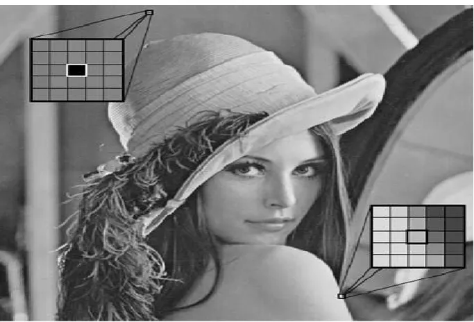
highest pixel luminance values within the dynamic range respectively. So that it is little bit difficult to remove random valued impulse noise rather than salt and pepper noise [Srinivasan, 2007]. The main difficulties which have to face for attenuation of noise is the preservation of image details. The difference between SPN and RVIN may be best described by Figure 1.3. In the case of SPN the pixel substitute in the form of noise may be either Lmin(0) or Lmax (255). Where as in RVIN situation it may range from Lminto Lmax. Cleaning such noise is far more difficult than cleaning fixed-valued impulse noise since for the latter, the differences in gray levels between a noisy pixel and its noise-free neighbors are significant most of the times. In this thesis, we focus only on random valued impulse noise (RVIN) and schemes are proposed to suppress RVIN.

Thesis Organization

The rest of the thesis is organized as follows. Chapter 2 describes about the image processing fundamentals details such as image Representation, Visualization, Discreatization, Restoration etc and different types of noises which causes image degradation, noise model, various filters used for noise removal, performance measures to identifying efficient filter. Chapter 3 describes about the related work and previous findings. Chapter 4 describes about noise detection mechanism (ROAD). And discusses about removal of noises using some standard filters etc. Chapter 5 proposes a new technique for denoising the random-valued impulsive noise. The proposed filter is based on rank ordered absolute difference. In the detection phase, basically, use the rank ordered absolute difference to distinguish between a noise or a image details. Implementation and details comparison with median and wiener filter BDND, BRBDNR, NUASM has been made. Chapter 6 represents simulation and experimental results. Chapter leads to a conclusion. An image may be defined as a two dimensional function, f(x, y), where x and y are spatial coordinates, and the amplitude of f at any pair of coordinates

(x, y) is called the intensity or gray level of the image at that point. When x, y and the amplitude values of f are all finite, discrete quantities, then the image can be called as a digital image. The field of digital image processing refers to processing digital images by means of a digital computer. Image restoration is a fundamental step of digital image processing [Gonzalez, 2007]. The entire process of image processing and analysis starting from the receiving of visual information to the giving out description of the scene, may be divided into three major stages which are also considered as major sub-areas, and are given below:

• Discretization and representation: converting visual information into a discrete form; suitable for computer processing; approximating visual information to save storage space as well as time requirement in subsequent processing.

• Processing: improving image quality by filtering etc.; compressing data to save storage and channel capacity during transmission.

• Analysis: extracting image features; quantifying shapes, registration and recognition.

• In the initial stage, the input is a scene (visual information), and the output is corresponding digital image. In the secondary stage, both the input and the output are images where the output is an improved version of the input. And, in the final stage, the input is still an image but the output is a description of the contents of that image [Chandra, 2007]. A schematic diagram of different stages is shown in Figure 1.1. The figure is taken from the book specified in [Chandra, 2007]. Out of the sub-branches of digital image processing, diagrammatically represented below, this thesis deals with image restoration. To be precise, the thesis devotes on a part of the image restoration i.e. noise removal from images. Accurately, it is about the denoising of one particular type of noise i.e. Impulsive noise, stated in the Problem Definition.

Image Restoration: Restoration attempts to reconstruct or recover an image that has been degraded by using a priori knowledge of the degradation phenomenon. Restoration techniques are primarily modeling of the degradation and applying the inverse process in order to recover the original image. The degradation function together with an additive noise operates on an input image f(x, y) to produce a degraded image g(x, y). Given g(x, y), some knowledge about the degradation function h(x, y) and some knowledge about the additive noise term η(x,y) the objective of restoration is to obtain an estimate of the original image [Gonzalez, 2007]. The degraded image is given in spatial domain by g(x, y) = f(x, y) * h(x, y) + η(x, y) (1.1) In this thesis, it is assumed that the degradation function is the identity operator, and it deals only with degradations due to noise. So the degraded image is:

g(x,y) = f(x,y ) + n(x,y) (1)

(3)

Figure 1: Representation of (a) Salt & Pepper Noise with Ri,j ∈ {nmin, nmax}, (b)Random Valued Impulsive Noise with Ri,j ∈ [nmin, nmax]

Fig 2. Different stages of image processing and analysis scheme

(4)

Fig 4. 1 local window information from Lena noisy image patch

Table 1. Median value calculation in local window example

123 125 126 130 140

122 124 126 127 135

118 120 150 125 134

119 115 119 123 133

111 116 110 120 130

Median value calculation 115,119,120,123, 124,125,126,127,150 Median value=124

(5)

Loosely, noise can be defined as any disturbance tending to interfere with the normal operation of a device or system. Image noise is a random, usually unwanted, variation in brightness or color information in an image [23]. Image noise can originate in film grain, or in electronic noise in the input device (scanner or digital camera) sensor and circuitry, or in the unavoidable shot noise of an ideal photon detector. Digital images are prone to a variety of types of noise. Noise is the result of errors in the image acquisition / transmission process that result in pixel values that do not reflect the true intensities of the real scene. There are several ways that noise can be introduced into an image, depending on how the image is created. For example: If the image is scanned from a photograph made on film, the film grain is a source of noise. Noise can also be the result of damage to the film [Dong, 2007], or be introduced by the scanner itself. If the image is acquired directly in a digital format, the mechanism for gathering the data (such as a CCD detector) can introduce noise. Electronic transmission of image data can introduces noise [Chandra, 2007]. The spatial component of noise is based on the statistical behavior of the intensity values. These may be considered as random variables, characterized by a probability density function (pdf). A probability density function (pdf), or density, of a random variable is a function which describes the density of probability at each point in the sample space. The probability of a random variable falling within a given set is given by the integral of its density over the set. Some commonly found noises are Gaussian noise, Rayleigh noise, Gamma noise, Exponential noise, Impulsive noise and so on.

Different types of noise: Noise in images is caused by the random fluctuations in brightness or color information. Noise represents unwanted information which degrades the image quality. Noise is defined as a process which affects the acquired image quality that is being not a part of the original image content [Charles Boncelet, 2005]. Digital image noise may occur due to various sources. During acquisition process, digital images convert optical signals into electrical one and then to digital signals and are one process by which the noise is introduced in digital images. Due to natural phenomena at conversion process each stage experiences a fluctuation that adds a random value to the intensity of a pixel in a resulting image. In general image noise is regarded as an undesirable by-product of image capture. In general image noise is regarded as anundesirable by-product of image capture.

The types of Noise are following

• Amplifier noise (Gaussian noise) • Salt-and-pepper noise

• Shot noise (Poisson noise)

Gaussian noise: Gaussian noise is statistical in nature. Its probability density function equal to that of normal distribution, which is otherwise called as Gaussian distribution. In this type of noise, values of that the noise are being Gaussian-distributed. A special case of Gaussian noise is white Gaussian noise, in which the values always are statistically independent. For application purpose, Gaussian noise is also used as additive white noise to produce additive white Gaussian noise. Gaussian noise is commonly defined as the noise with a Gaussian amplitude distribution, which states that nothing the correlation of the noise in time or the spectral

density of noise. Gaussian noise is otherwise said as white noise which describes the correlation of noise. Gaussian noise is sometimes equated to be of white Gaussian noise, but it may not necessarily the case.

Salt and pepper noise: In [Charles Boncelet, 2005; Chen, 2008], salt & pepper noise model, there is only two possible values ‘a’ and ‘b. The probability of getting each of them is less than 0.1 (else, the noise would greatly dominate the image). For 8 bit/pixel image, the intensity value for pepper noise typically found nearer to 0 and for salt noise it is near to 255. Salt and pepper noise is a generalized form of noise typically seen in images. In image criteria the noise itself represents as randomly occurring white and black pixels. An effective noise reduction algorithm for this type of noise involves the usage of a median filter, morphological filter. Salt and pepper noise occurs in images under situations where quick transients, such as faulty switching take place. This type of noise can be caused by malfunctioning of analog-to-digital converter in cameras, bit errors in transmission, etc.

Poisson noise: Poisson noise is also known as [44] shot noise. It is a type of electronic noise. Poisson noise occur under the situations where there is a statistical fluctuations in the measurement caused either due to finite number of particles like electron in an electronic circuit that carry energy, or by the photons in an optical device

Speckle noise: In [Charles Boncelet, 2005; Rosa-Zurera,

2007; Sedef Kent et al., 2004], Speckle noise is a type of granular noise that commonly exists in and causes degradation in the image quality. Speckle noise tends to damage the image being acquired from the active radar as well as synthetic aperture radar (SAR) images. Due to random fluctuations in the return signal from an object in conventional radar that is not big as single image-processing element. Speckle noise occurs. Speckle noise increases the mean grey level of a local area. Speckle noise is more serious issue, causing difficulties for image interpretation in SAR images. It is mainly due to coherent processing of backscattered signals from multiple distributed targets.

Spatial filtering: Spatial filtering is preferred when only additive noise is present. The different classes of filtering techniques exist in spatial domain filtering.

• Mean Filter

• Order-Statistics Filter • Adaptive Filter

(6)

The arithmetic and geometric mean filters are well suited for random noise like Gaussian or uniform noise. The contra harmonic filter is well suited for impulsive noise [Gonzalez, 2007].

Order-Statistics Filter: Order statistics (OS) are the

characteristics of sorted data within a sliding window. The minimum, maximum and median are special cases of order statistics. Order statistics are extremely robust to outlier data and are used when outlier data is problematic. Order Statistics filters are nonlinear and nonstationary (shiftvariant). Order -statistics filters are spatial filters whose response is based on ordering (ranking) the pixels contained in the image area encompassed by the filter. The response of the filter at any point is determined by the ranking result. Median filter, Max and min filters, Midpoint filter Alpha-trimmed mean filter are some of the order-statistics filter. Median filter replaces the value of a pixel by the median of the gray levels in the neighborhood of that pixel. Pixel value is replaced by minimum and maximum gray levels of the window respectively for min and max filter. The midpoint filter simply computes the midpoint between the maximum and minimum values in the area encompassed by the filter. Median filters are particularly effective in the presence of impulse noise [Gonzalez, 2007].

Adaptive Filter: Adaptive filters change its behavior based on the statistical characteristics of the image inside the filter window. Adaptive filter performance is usually superior to non-adaptive counterparts. But the improved performance is at the cost of added filter complexity. Mean and variance are two important statistical measures using which adaptive filters can be designed. For example if the local variance is high compared to the overall image variance, the filter should return a value close to the present value. Because high variance is usually associated with edges and edges should be preserved. Adaptive, local noise reduction filter and adaptive median filter are the example of adaptive filter [Gonzalez, 2007].

Performance Measures: The metric used for performance

comparison of different filters are defined below.

Mean Squared Error (MSE) and Peak Signal to Noise Ratio (PSNR): In statistics, the mean squared error or MSE of an estimator is one of many ways to quantify the amount by which an estimator differs from the true value of the quantity being estimated. Here it is just used to calculate the difference between a original image with a restored image. PSNR analysis uses a standard mathematical model to measure an objective difference between two images. It estimates the quality of a reconstructed image with respect to an original image. The basic idea is to compute a single number that reflects the quality of the reconstructed image. Reconstructed images with higher PSNR are judged better.

Given an original image Y of size (M × N) pixels and a reconstructed image Ŷ the PSNR (dB) is defined as:

PSNR (dB)=10log10 (2)

MSE= (3)

Image enhancement factor (IEF): Image enhancement is to improve the interpretability or perception of information in images for human viewers, or to provide `better' input for other automated image processing techniques. Image enhancement techniques can be divided into two broad categories:

• Spatial domain methods, which operate directly on pixels, and

• Frequency domain methods, which operate on the Fourier transform of an image.

IEF = (4)

Structural Similarity Index (SSIM): The Structural

Similarity Index (SSIM) is a perceptual metric that

quantifies image quality degradation caused

by processing such as data compression or by losses in data transmission. It is a full reference metric that requires

two images from the same image capture a

reference image and a processed image.

Feature similarity index(FSIM): Feature similarity index is a measurement used in image processing to verify feature Similarity after restoration image from the degraded one.

Subjective or Qualitative measure: Along with the above performance measure subjective assessment is also required to measure the image quality. In a subjective assessment measures characteristics of human perception become paramount, and image quality is correlated with the preference of an observer or the performance of an operator for some specific task. However perceptual quality evaluation is not a deterministic process.

(7)

Filtering mechanism is applied only to the noisy pixels. Removal of the random-valued impulse noise is done by two stages: detection of noisy pixel and replacement of that pixel. Median filter is used as a backbone for removal of impulse noise. Many filters with an impulse detector are proposed to remove impulse noise. T. Chen et.al has suggested Adaptive center weighted median (ACWM) [Chen, 2001] which is a novel adaptive operator, that forms estimates based on the differences between the current pixel and the outputs of center-weighted median (CWM) [Ko, 1991] filters with varied center weights. It employs the switching scheme based on the impulse detection mechanisms. It utilizes the center-weighted median filter that have varied center weights to define a more general operator, which realizes the impulse detection by using the differences defined between the outputs of CWM filters and the current pixel of concern. The ultimate output is switched between the median and the current pixel itself. T. Chen et.al has suggested a generalized framework of median based switching schemes, called multi-state median (MSM) [Chen, 2001] filter. By using simple threshold logic, the output of the MSM filter is adaptively switched among those of a group of center weighted median (CWM) filters that have different center weights. The MSM filter is equivalent to an adaptive CWM filter with a space varying center weight which is dependent on local signal statistics. K. Ma T. Chen proposed Tri-State Median Filter (TSM) [Ma, 1999] for preserving image details while effectively suppressing impulse noise. It incorporates the standard median(SM) filter and the center weighted median (CWM) filter into a noise detection framework to determine whether a pixel is corrupted, before applying filtering unconditionally. Noise detection is realized by an impulse detector, which takes the outputs from the SM and CWM filters and compares them with the origin or center pixel value in order to make a tri-state decision. The switching logic is controlled by a threshold. The threshold affects the performance of impulse detection. An attractive merit of the TSM filter is that it provides an adaptive decision to detect local noise simply based on the outputs of these filters. V. Senk et.al proposed Advanced Impulse Detection Based on Pixel-Wise MAD (PWMAD) [Senk, 2004] a robust estimator of variance, MAD (median of the absolute deviations from the median), is modified and used to efficiently separate noisy pixels from the image details.

The algorithm is free of varying parameters, requires no previous training or optimization, and successfully removes all type of impulse noise. The pixel-wise MAD concept is straightforward and low in complexity. The median of the absolute deviations from the median-MAD is used to estimate the presence of image details, thus providing their efficient separation from noisy image pixels. An iterative pixel-wise modification of MAD (PWMAD) provides reliable removal of arbitrarily distributed impulse noises. K. Mitra et.al proposed Signal-Dependent Rank Order Mean (SDROM) Filter [9] which is a new framework for removing impulse noise from images, in which the nature of the filtering operation is conditioned on a state variable defined as the output of a classifier that operates on the differences between the input pixel and the remaining rank-ordered pixels in a sliding window. First, a simple two-state approach is described in which the algorithm switches between the output of an identity filter and a rank-ordered mean (ROM) filter. The technique achieves an excellent tradeoff between noise suppression and detail preservation with little increase in computational

complexity over the simple median filter. For a small additional cost in memory, this simple strategy is easily generalized into a multistate approach using weighted combinations of the identity and ROM filter in which the weighting coefficients can be optimized using image training data. Moreover, the method can effectively restore images corrupted with Gaussian noise and mixed Gaussian and im pulse noise. Y.Dong et.al suggested another method for removal of random-valued impulse noise is directional weighted med ian filter (DWM) [Dong, 2007]. This filter uses a new impulse detector, which is based on the differences between the current pixel and its neighbors aligned with four main directions. After impulse detection, it does not simply replace noisy pixels identified by outputs of median filter but continue to use the information of the four directions to weight the pixels in the window in order to preserve the details as removing noise. First it considers a 5X5 window. Now it considers the four directions: horizontal, vertical and two diagonal. Each direction there is 5 pixel points. It then calculates the weighted difference in each direction and takes the minimum of them.

(8)

The different steps involved in the BDND algorithm are explained in the above section. The noise filtering stage uses the Modified Noise Adaptive Switching Filter for removing the uncorrupted pixels within the image. Sruthi Ignatious et.al suggested the Iterative Average Estimation Filter (IAEF) [Sruthi Ignatious, 2013] using BDND algorithm consists of two stages, such as Noise Detection stage and Noise filtering stage. The noise detection stage uses Boundary Discriminative Noise Detection (BDND) algorithm for identifying the noisy pixels within the image. The noise filtering stage uses average estimated value of the uncorrupted pixels and replaces the corrupted pixel with the estimated value.

This filtering technique consumes less time. Ng, P.-E., Ma, K.-K., et.al suggested witching Median Filter [Ng, 2006], the filtering will be done based on some threshold value. This threshold value selection depends on the noise density within the filtering window. The major drawback of this filtering technique is that it is difficult to define the threshold value. Also this technique will not preserve the edge details when the noise density is high. H. Hwang et.al suggested Adaptive median filter AMF [Hwang, 1995].Median filter based on the statistical characteristics of the image is considered as Best for filtering images.

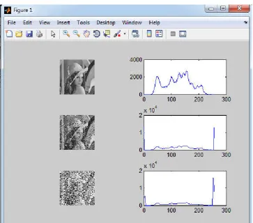
Figure 6. Noise models with histogram

Table 2. Performance analysis of median filter

i/p image Noise density MSE SSIM PSNR Lena 10 3.0908 0.9779 36.2991

20 6.16 0.9176 29.945

30 10.3543 0.7412 23.8222 40 17.7079 0.4581 18.9251 50 28.1170 0.2276 15.1905 60 42.9959 0.1042 12.2415 70 60.4952 0.0526 9.9942 80 81.2169 0.0248 8.1140 90 104.7713 0.0122 6.6096

Table 3. Performance analysis of Weiner filter

i/p image Noise density MSE SSIM PSNR

Lena 10 9.8691 0.6321 23.6086

20 18.6135 0.5268 22.0548

30 30.5002 0.4206 20.1233

40 47.4174 0.2952 17.8521

50 67.2593 0.1727 15.3277

60 86.7699 0.0929 13.0546

70 101.2980 0.0441 11.1186 80 110.9957 0.0240 9.4779

(9)

Fig 7. Median filter filtration

Fig 8. Weiner filter result

(10)

AMF works well for SPN removal even at high noise level. However there are two drawbacks. The first one is that AMF may cause error in noise detection. For example, if the center pixel value equals to the non-local maximum (or minimum) value of its window but not salt or pepper noise, it would still be regarded as noise candidate by in AMF algorithm. Another drawback of AMF is that for very high level of noise, the recovered image may lose many details and edge detection.

To overcome these drawbacks of AMF and enhance the image restoration quality, AWMF is introduced by Peixuan Zhang et.al to enhance the performance of denoising, based on the working mechanism of AMF filter, the main idea of AWMF is to decrease the detection errors and to replace the noise candidates by better value than median. After noise detection, in AWMF method, the noise candidate is replaced by the Fig 10. Comparison result of SSIM

(11)

Noisy Image

Table 4.Comparative data analysis of false alarm in different filters

Filter BRBDNR

Noise density (%) False alarm(FA)

10 29220

20 17857

30 9297

40 3737

50 1640

60 2964

Table 5.Comparative data analysis of missed detection in different filters

Filter BRBDNR

Noise density (%) Missed Detection (MD)

10 65

20 557

30 3141

40 18427

50 55788

60 99290

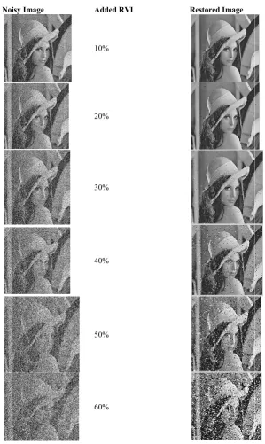
Added RVI Restored Image

10%

20%

30%

40%

50%

60%

Fig 13.Shows the input and output image

Table 4.Comparative data analysis of false alarm in different filters

BDND NUASAM

False alarm(FA)

6350 1034

9475 1164

17538 1302

32082 1881

49010 3889

61012 8539

BDND NUASAM

Detection (MD)

46 1640

531 3365

2697 5108

8110 7554

18608 11720

35840 19539

Proposed

7 6 10 22 20 32

Proposed

(12)

weighted mean value of the current window while the noise-free pixel is left unchanged. The weighted mean in AWMF is a better choice than the median in AMF to replace the noisy candidate especially for high levels of noise. There are two reasons for us to possible noisy pixels while in AMF the output median includes the effect of them. Secondly, experimental comparison has been done in [Peixuan, 2014] which show that the PSNR of image, in which noise candidates are replaced by weighted mean values, is higher than that of weighted median values on average. Switching non-local means filter (SNLM) [Nasri, ?] One of the most important and powerful methods proposed by M. Nasri et.al which considers all the image information to restore a noisy image is the non-local means (NLM) filter. The NLM is integrated to a switching framework, and a switching Non-local means filter SNLM [Nasri et al., ?] is proposed for removal of impulse noise, especially in HDIN(>70%) reduction [Zhou et al., 1999]. In first stage noise pixels are detected, based on the fact that their values must be the extreme gray level of the image. Then the image is restored, based on noise-free pixels in a non-local manner. In the SNP case, BDND [Iyad F.Jafar et al., ?] and simple detection [Srinivasan, 2007; Esakki rajan, 2011] are examples of effective impulse detectors. Iyad F. Jafar et.al proposed Boundary discriminative noise detection (BDND)[19] Switching median filters are known to outperform standard median filters in the removal of impulse noise due to their capability of filtering candidate noisy pixels and leaving other pixels intact.

The boundary discriminative noise detection (BDND) is one powerful example in this class of filters. The BDND filter is proven to operate efficiently when compared to other filters, even under high noise densities (up to 90%). Being a switching-based median filter, the BDND algorithm filters the noisy image in two steps. The first step is essentially a noise detection step which is based on clustering the pixels in the image in a localized window into three groups, namely; lower intensity impulse noise, uncorrupted pixels, and higher intensity impulse noise. The clustering is based on defining two boundaries using the intensity differences in the ordered set of the pixels in the window. The pixel is classified as uncorrupted if it belongs to the middle cluster. Otherwise it is a noisy pixel. Once the noise map is determined, the second step is the filtering step, which is supposed to replace the noisy pixel with an estimate of its original value. This step is applied on the identified noisy pixels only. The filtering is essentially a median filtering operation that is applied on the uncorrupted pixels found in the filtering window. The critical parameter that is required to be defined in the filtering step of the BDND algorithm is the size of the filtering window. Xiaotian Wanget.al proposed Non-uniform sampling and autoregressive modeling [Xiaotian Wang1 et al., ?]. The challenge of image impulse noise removal is to restore spatial details from damaged pixels using remaining ones in random locations. Most existing methods use all uncontaminated pixels within a local window to estimate the centered noisy one via a statistic way.

Table 6. PSNR (Peak signal to noise ratio comparison among filters)

Noise density BRBDNR BDND NUASM Proposed 10 34.90982 35.33848 34.90982 42.93883 20 32.90524 30.72783 32.90524 39.5 30 27.04175 24.67717 27.04175 37.26798 40 19.17641 19.16315 19.17641 35.55494 50 14.15022 14.4636 14.15022 33.74834 60 11.34043 10.9053 11.34043 30.55413

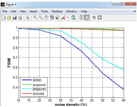
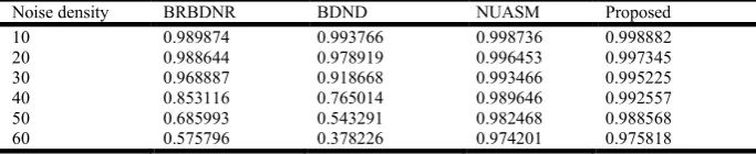
Table 7. Comparison of FSIM among different filters

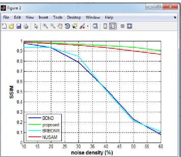
Table 8. Comparison of SSIM among different filters

Table 9. Comparison of IEF among different filters

Noise density BRBDNR BDND NUASM Proposed

10 82.83621 91.42949 475.0165 526.1635

20 104.7268 63.43329 322.9585 478.1167

30 40.75652 23.64497 271.2395 429.3576

40 8.873357 8.846293 225.9056 385.4253

50 3.483695 3.744366 168.8007 317.5797

(13)

These kinds of methods have two defects. First, all noisy pixels are treated as independent individuals and estimated by their neighbors one by one, with the correlation between their true values ignored. Second, the image structure as a natural feature is usually ignored. This study proposes a new denoising framework, in which all noisy pixels are jointly restored via non-uniform sampling and supervised piecewise autoregressive modeling based super-resolution. In this method, the noisy pixels are jointly estimated in groups through solving a well-designed optimization problem, in which image structure feature is considered as an important constraint. Cheng-suing hsiehet.al proposed Boundary resetting boundary discriminative noise detection (BRBDNR) [Cheng-hsiung hsieh, ?] in which image restoration approach, two stages are involved: noise detection and noise replacement. The BRBDNR is used to detect noisy pixels in an image. If a pixel is uncorrupted, then keep it intact. Or replace it with an uncorrupted neighborhood pixel through the MFSW. Note that miss detection happens in the BDND presented in [Iyad, ?; Ng et al., 2006] when the noise density is high. The miss detection is even worse for cases with unbalanced noisy density where the portions for the salt noise and the pepper noise are different. A boundary resetting scheme is incorporated into the BDND. By this doing, the problem of miss detection described above can be prevented. BRBDND/MFSW generally outperforms the BDND/MNASM both in the PSNR and the visual quality of restored image.

Noise Detection and Removal

Random valued impulsive noise removal using noise

detection scheme: The main challenge in impulse noise

removal is to suppress the noise as well as to preserve the details (edges). Removal of the random-valued impulse noise is done by two stages: detection of noisy pixel and replacement of that pixel. Median filter is used as a backbone for removal of impulse noise. Many filters with an impulse detector are proposed to remove impulse noise; some of them are described in the previous chapter. Here a new approach for removal of random-valued impulsive noise from images is suggested. The scheme works in two phases, namely a novel detection of contaminated pixels followed by the filtering of only those pixels keeping others intact. The detection scheme utilizes rank order absolute difference of pixels in a test window and the filtering scheme is a variation median filter based and means based mechanism.

Rank Ordered absolute Difference: ROAD scheme

employed to generate a cleaner reference variable for detecting noise. One crucial problem for IN removal is the noise detection. Most existing IN detectors can be classified into two types. One is based on the absolute deviation

d (xi,j) =| xi,j - Ωi,j | (5)

Where Ωi,j denotes the reference variable calculated from the

local information. This absolute deviation is further compared with an appropriate threshold T. Then a binary matrix f is chosen to record the compared results.

(6)

Where the value ‘‘1’’ means that the current pixel xi,j is a noisy

pixel, otherwise xi,j is a clean pixel.

Over the years, various local statistics are used as the reference variables. For example, ( is replaced by the median or weighted median in [Luo, 2005; Sun, 1994; Xiong, 2012], normalized mean in [Florencio, 1994], rank order in [Abreu, 1996], center-weighted median in [Ko, 1991], median of the absolute deviations from the median (MAD) in [Senk, 2004], directional weighted median in [Dong, 2007], weighted mean in [Akkoul, 2010], and median of sorted quadrant median vector (SQMV) in [Lin, 2010]. The other one is based on the absolute differences between the center pixel and its neighbors. Denote xk,l be the neighbor pixels of xi,j within a

local window, then the absolute difference is defined by,

di,j(k,l)=| xi,j – xk,l |

(7)

A typical representative of such detection scheme is the rank-ordered absolute difference (ROAD) [Garnett, 2005].

ROAD m (xi,j)= (8)

Where defined

in Eq. The ROAD value, which may be used to compare with a threshold, provides a proximity measurement between a pixel and its m most similar neighbors. Later, taking the logarithm of the absolute difference, Dong et al. [2007] proposed a statistic ROLD to improve the detection accuracy. Employing a reference image, Yu et al. [2008] introduced a rank-ordered relative difference (RORD) which can preserve more image edges than ROAD and ROLD. In [Ghanekar, 2010], Ghanehar et al. used an exponential function to enlarge

the absolute difference in , and identify noise in a similar way with ROAD scheme. The basic assumption of ROAD is it assumes that the ROAD values of noisy pixels always larger than those of clean ones.

(14)

Such strategy is further improved by the new ACWM in and the adaptive weighted mean filter (AWMF) in Zhang and Fang, 2014]. In [Ghanekar, 2010

enhancement-based filter (CEF) is presented, where the absolute differences are first enlarged by an exponential function and then summed to identify noisy pixels. The noisy pixels were further filtered by the weighted median filter. noisy pixels were further filtered by the weighted median filter. Tsai et al. [36] employed ten existing

construct a two-level tree for noisy pixels detection, and the noisy pixels were restored by a median-type filter associated with the support vector regression method. Recent years, some mean filters were also incorporated into the switchin

for IN removal as they can capture more image detailed information. In [Garnett et al., 2005], the statistic

incorporated into the bilateral filter and a trilateral filter was designed for IN reduction. In [Tsai et al., 2012

arithmetic mean filter was combined with a detector to remove IN. Lin et al. [2010] presented a switching bilateral filter to suppress IN. Recently, united with detectors, the non mean (NLM) filer [Buades, 2005] was also extended for IN removal due to its fantastic denoising performance

2012; Hu, 2014]. In [Xiong, 2012], the weights of NLM were calculated on an initial denoised image, while these in were[39] computed on the noisy image by diminishing the contributions of noisy pixels offered in the similarity measurement calculation. Combining the noise detector into distance learning, Delon et al. [2013]proposed a patch based method for IN removal.

Median filter: Median filter is the nonlinear filter.

idea behind the median filter is to find the median value by across the window, replacing each entry in the window with the median value of the pixel

[James, 2008]. The pattern of neighbor’s pixels is called the “window", when the window contains odd number of values in it then the median is simple: it is just the center value after all the entries in the window are sorted numerically in ascending order. But for an even number of entries, there is more than one center value; in that case the average of the two center pixel values is used. One of the major problems with the median filter is that it is relatively expensive and complex computation. For finding the median it is necessary to sort all the values in the neighborhood into numerical order an filter relatively slow, even it is performed with fast sorting algorithms like quick sort. However the basic algorithm can be enhanced somewhat for the speed purpose.

Weiner filter: The main aim of the Wiener filter [

2000] is to filter out the image that has been corrupted by noise. Wiener filter is based on a statistical approach. Desired frequency response can be acquired using this filter. Approaches followed by wiener filtering are of different angle. For performing filtering operation it is must to have knowledge of the spectral properties of the original signal and the noise, in achieving the criteria one can get the LTI filter whose output will be as close as original signal as possible. Wiener filters possess characterized by the following:

Assumption: signal and (additive) noise are stationary linear random processes with known spectral characteristics. b. Requirement: the filter must be causal where this requirement is failed it resulting in a non-causal solution Periodic noise be effectively removed by correcting the amplitude spectrum Such strategy is further improved by the new ACWM in [4] and the adaptive weighted mean filter (AWMF) in [Peixuan

, 2010], a contrast based filter (CEF) is presented, where the nlarged by an exponential function and then summed to identify noisy pixels. The noisy pixels were further filtered by the weighted median filter. The noisy pixels were further filtered by the weighted median employed ten existing IN detectors to level tree for noisy pixels detection, and the type filter associated with the support vector regression method. Recent years, some mean filters were also incorporated into the switching scheme for IN removal as they can capture more image detailed statistic ROAD was incorporated into the bilateral filter and a trilateral filter was 2012], a rank-ordered arithmetic mean filter was combined with a detector to remove presented a switching bilateral filter to suppress IN. Recently, united with detectors, the non-local was also extended for IN removal due to its fantastic denoising performance [Xiong, ], the weights of NLM were calculated on an initial denoised image, while these in computed on the noisy image by diminishing the ontributions of noisy pixels offered in the similarity measurement calculation. Combining the noise detector into proposed a patch based

Median filter is the nonlinear filter. The main idea behind the median filter is to find the median value by across the window, replacing each entry in the window with

The pattern of neighbor’s pixels is called the odd number of values in it then the median is simple: it is just the center value after all the entries in the window are sorted numerically in ascending order. But for an even number of entries, there is more than e of the two center pixel values is used. One of the major problems with the median filter is that it is relatively expensive and complex computation. For finding the median it is necessary to sort all the values in the neighborhood into numerical order and this filter relatively slow, even it is performed with fast sorting algorithms like quick sort. However the basic algorithm can be

The main aim of the Wiener filter [Shi Zhong, out the image that has been corrupted by noise. Wiener filter is based on a statistical approach. Desired frequency response can be acquired using this filter. Approaches followed by wiener filtering are of different angle. on it is must to have knowledge of the spectral properties of the original signal and the noise, in achieving the criteria one can get the LTI filter whose output will be as close as original signal as possible.

following:

signal and (additive) noise are stationary linear random processes with known spectral characteristics. b. Requirement: the filter must be causal where this requirement causal solution Periodic noise can be effectively removed by correcting the amplitude spectrum

components altered by the noise, and two frequency filtering methods are currently available, i.e., Wiener filtering and notch filtering. However, a Wiener filter requires an accurate noise model, which may be difficult to obtain in various practical cases. In addition, a Wiener filter is also complicated in computation

Mean filter: There are two types of filtering schemes namely

linear filtering and nonlinear filtering. [

Mean filter comes under linear filtering scheme. Mean filter is also known as averaging filter. The Mean Filter applies mask over each pixel in the signal. Each of the components of the pixels comes under the mask are being averaged together to form a single pixel that is why the filter is otherwise known as average filter. Edge preserving criteria is poor in mean filter. Mean filter is defined by

Mean filter (X1……XN….) = ∑

Where (x1 ….. xN) is image pixel range. Mean filter is useful for removing grain noise from the photography image. As each pixel gets summed the average of the pixels in its neighborhood is found out, local variations caused by grain noise are reduced considerably by replacing it with average value. Here first an input imag

in that image. To identifying the noise candidate detection mechanism is used. After identifying the noise candidates the proposed filter is used for filtering the noisy candidates which is to be used to restore the noisy ca

restored image.

Proposed modified weighted mean filter

the next problem is how to choose an appropriate filter to remove these detected noisy pixels. Instead of using the existing median or mean filters [

2012] proposed by F. Ahmed et.al, B.xiong et.al

section a more robust weighted mean filter (MWMF) is designed for image denoising. The weight in the proposed MWMF contains three components which take into account both the image features and IN characteristics. Hence it is more suitable for IN removal.

coordinates within a (2N+1) centered at the (i,j)-th pixel. Suppose x

the noisy image, and is the

=

Where is the distance weight inverse to the spatial

distance between the neighbor pixel (i.e.,

one (i.e., ). It is expected that the larger the distance

between and is, the smaller the distan

should be, and vice versa. Here, inverse function of the spatial distance

=

is called clean-like weight, which means that if a pixel is more likely to be a clean pixel, then it should be matched with components altered by the noise, and two frequency filtering methods are currently available, i.e., Wiener filtering and notch filtering. However, a Wiener filter requires an accurate del, which may be difficult to obtain in various practical cases. In addition, a Wiener filter is also complicated

There are two types of filtering schemes namely linear filtering and nonlinear filtering. [Gajanand Gupta, 2011] Mean filter comes under linear filtering scheme. Mean filter is also known as averaging filter. The Mean Filter applies mask over each pixel in the signal. Each of the components of the pixels comes under the mask are being averaged together to gle pixel that is why the filter is otherwise known as average filter. Edge preserving criteria is poor in mean filter.

) is image pixel range. Mean filter is useful oving grain noise from the photography image. As each pixel gets summed the average of the pixels in its neighborhood is found out, local variations caused by grain noise are reduced considerably by replacing it with average Here first an input image is taken. Then noise is added To identifying the noise candidate detection After identifying the noise candidates the proposed filter is used for filtering the noisy candidates which is to be used to restore the noisy candidates to obtain the

Proposed modified weighted mean filter: After detection, the next problem is how to choose an appropriate filter to remove these detected noisy pixels. Instead of using the existing median or mean filters [Ahmed, 2014; Xiong et al., F. Ahmed et.al, B.xiong et.al, in this a more robust weighted mean filter (MWMF) is designed for image denoising. The weight in the proposed MWMF contains three components which take into account e features and IN characteristics. Hence it is more suitable for IN removal. Let Si,j be a set of pixel

coordinates within a (2N+1) × (2N+1) sliding window, th pixel. Suppose xi,j is the (i,j)-th pixel in

is the output of the filter, then

(9)

is the distance weight inverse to the spatial

distance between the neighbor pixel (i.e., ) and the center

). It is expected that the larger the distance

is, the smaller the distance weight

should be, and vice versa. Here, is simply defined as the inverse function of the spatial distance

(10)

(15)

a higher weight. On the contrast, if a pixel has a larger probability to be noise, the clean-like weight for it should be lower. Extremely, the noise free pixel has the largest weight, and the completely noisy pixel (the pixel with f value equals to 1) has no weight. Therefore, the clean-like weight is defined as,

=

(11)

And is the median-similarity weight, which indicates that

if the luminance intensity of is closer to the median value of the relative-clean pixels (pixels with membership function f

< 1), the median-similarity weight for should be higher. The mathematical formula is defined as follows

= (12)

in which is the neighbor pixel of in

the sliding window, is the median value of the neighbor

pixels excluded the noisy ones, i.e. , denotes the set containing the relative clean pixels in the window.

(13)

And =max { }

is the maximum difference

The idea for designing such three components for the weight is quite simple. Firstly, it is well known that, in natural images, the closer the distance of two pixels is, the closer the relationship will be. Hence setting larger weights for these pixels that near to the current pixel is reasonable. Secondly, it is sensible just using these information pixels to filtering the noisy ones. Therefore, in the proposed weighted mean filter,

the clean-like weight is inversely proportional to the membership function f. Finally, since median value is a good estimator for the IN, it is advisable to design large weights for these pixels whose luminance intensities are approach to the median value of the relative-clean ones.

Proposed Denoising algorithm: All the pixels in the image undergo testing for noise detection. A binary decision matrix is formed at the end of calculation. The decision matrix has values ‘1’ indicating corrupted and ‘0’ as uncorrupted. Further filtration of noisy pixels is done by storing value of X̂ in x(i,j) The size of input image X is denoted as P*Q. restored image Y.

Algorithm 1

1. Read noisy image X.

2. Initialize N=1,Threshold T=60; 3. For every row i= 1 to P 4. For every column j= 1 to Q

5. Create rectangular 3×3 window around the noisy pixel and find ROAD values and compare with

threshold T, update the binary noise matrix f.

6. End for column 7. End for row

8. for every row i=1 to P 9. for every col j=1 to Q 10. if X(i,j)==1

11. ifN<Nmax && <3 minimum clean pixel

12. X (row, col)= X̂ (i,j) 13. else

14. N=N+1 15. end if 16. end if

17. end for column 18. end for row

Simulation and Experimental Results: The simulation was

carried out using MATLAB (Matrix laboratory) of R2014 version (8.3.0.532).Simulation work is implemented in windows-7 Home basic operating system, Intel(R) core(TM) i5 processor with processor speed 2.40 GHz, RAM 4 GB.

Parameter requirement: Threshold value (T=60)

Local window (2N+1) × (2N+1) Noise probability density (10-60%) Lena image

Figure 5 shows Lena image used as input image added with some amount of noise density, detection process and noise candidate identification process. Figure 6 shows Lena image as a input image added with 10% salt & pepper noise, detection is done by ROAD then filtered by standard median filter and its Histogrammatical representation. Figure 7 shows Lena image as an input image added with 10% salt & pepper noise, detection is done by ROAD then filtered by Weiner filter and its Histogrammatical representation.

Conclusion

An image is an artifact that depicts visual perception. A digital

image is a numeric representation (normally binary) of a

two-dimensional image. Noise is the unwanted information present

(16)

REFERENCES

Abreu, E., Lightstone, M., Mitra, S.K., Arakawa, K. 1996. A new efficient approach for the removal of impulse noise from highly corrupted images, IEEE Trans. Image Process. 5 (6) 012–1025.

Ahmed, F., Das, S. 2014. Removal of high-density salt-and-pepper noise in images with an iterative adaptive fuzzy filter using alpha-trimmed mean, IEEE512 Trans. Fuzzy Syst. 22 (5) 1352–1358.

Akkoul, S., Ledee, R., Leconge, R., Harba, R. 2010. A new adaptive switching median filter, IEEE Signal Process. Lett. 17 (6) 587–590.

Bovik, A.C. 2000. Hand book of Image and Video Processing. New York, NY, USA: Academic

Buades, A., Coll, B., Morel, J.M. 2005. A non-local algorithm for image denoising, in: IEEE Computer Society Conference on Computer Vision and Pattern Recognition, CVPR 2005, vol. 2, IEEE, pp. 60–65.

Chandra, B. and Dutta Majumder. D. 2007. Digital Image Processing and Analysis. Prentice-Hall, India, first edition. Charles Boncelet, “Image Noise Models” in Alan C.Bovik,

Handbook of Image and Video Processing, 2005

Chen T. and Wu. H. R. 2001. Space variant median filters for the restoration of impulse noise corrupted images. IEEE Trans. Circuits Syst. II, 48(8):784–789, August.

Chen, P.Y., Lien, C.Y. 2008. “An efficient edge-preserving algorithm for removal of salt-and-pepper noise”, IEEE Signal Processing Letters 15, 833–836.

Chen, T. and Wu. H. R. 2001. Adaptive impulse detection using center-weighted median filters. IEEE Signal Process. Lett., 8(1):1–3, January.

Cheng-hsiung hsieh, Po-chin huang, and Sheng-yung hung,” Noisy Image Restoration Based on Boundary Resetting BDND and Median Filtering with Smallest Window” Department of Computer Science and Information Engineering Chaoyang University of Technology

Delon, J., Desolneux, A. 2013. A patch-based approach for removing impulse or mixed gaussian-impulse noise, SIAM J. Imaging Sci. 6 (2) 1140–1174.

Dong, Y. and Xu. S. 2007. A new directional weighted median filter for removal of random-valued impulse noise. IEEE Signal Process. Lett, 14(3):193–196, March.

Dong, Y., Chan, R.H and Xu, S. 2007. “A detection statistics for random –valued impulse noise,”IEEE Transanctions on image processing, 16(4),pp 1112-1120.

Esakki Rajan, S, Veerakumar, T., Subramanyam, A.N and Premchand, C.H. 2011. “Removal of high density salt and peepper noise through modified decision based unsymmetric median filter”,IEEE signal processing letters,18(5),pp.287-29.

Esakkirajan, S., Veerakumar, T. 2011. Adabala N. Subramanyam, C.H. Prem Chand, “Removal of High density Salt and Pepper Noise Through Modified Decision Based Unsymmetric Trimmed Median Filter,” IEEE Signal process. Lett., Vol. 18,no 5,May

Florencio, D.A.F., Schafer, R.W. 1994. Decision-based median filter using local signal statistic, Proc. SPIE 2308 268–275.

G.Shi Zhong, 2000. “Image De-noising using Wavelet Thresholding and Model Selection”,Image Processing, 2000, Proceedings, International Conference on, Volume: 3, 10-13

Gajanand Gupta, 2011. “Algorithm for Image Processing Using Improved Median Filter andComparison of Mean, Median and Improved Median Filter” (IJSCE) ISSN: 2231-2307,Volume-1, Issue-5, November.

Garnett, R., Huegerich, T., Chui, C., He, W. 2005. A universal noise removal algorithm with an impulse detector, IEEE Trans. Image Process. 14 (11) 1747– 1754.

Ghanekar, U., Singh, A.K., Pandey, R. 2010. A contrast enhancement-based filter for removal of random valued impulse noise, IEEE Signal Process. Lett. 17 (1) 536 47– 50.

Gonzalez, R C and Woods. R E 2007. Digital Image Processing. Prentice-Hall, India, second edition.

H. Hwang and R.A. 1995. Haddad, “Adaptive median filters: New algorithms and results,” IEEE Trans. Image Process., vol. 4, no. 4, pp. 499–502.

Hu, H., Li, B., Liu, Q. 2014. Removing mixture of gaussian and impulse noise by patch-based weighted means, arXiv preprint arXiv:1403.2482.

Iyad F. Jafar, Rami A. AlNa’mneh and Khalid A. 2013. Darabkh, “Efficient Improvements on the BDND Filtering Algorithm for the Removal of High-Density Impulse Noise,” IEEE Transactions on Image Processing, vol.22, No. 3, (1223-1232). March.

Iyad F. Jafar, Rami A. AlNa’mneh, and Khalid A. Darabkh, Efficient Improvements on the BDND Filtering Algorithm for the Removal of High-Density Impulse Noise”

James C. Church, Yixin Chen, and Stephen V. 2008. Rice Department of Computer and Information Science, University of Mississippi, “A Spatial Median Filter for Noise Removal in Digital Images”, IEEE, page(s): 618- 623.

Ko, J., Lee, Y.H. 1991. Center weighted median filters and their applications to image enhancement, IEEE Trans. Circ. Syst. 38 (9) 984–993.

Lin, J.S. Tsai, C.T. Chiu, Switching bilateral filter with a texture/noise detector for universal noise removal, IEEE Trans. Image Process. 19 (9) (2010) 2307–2320.

Lin, T.C. 2007. A new adaptive center weighted median filter for suppressing impulsive noise in images, Inf. Sci. 177 (4) 1073–1087.

Lin, T.C. 2010. Switching-based filter based on dempsters combination rule for image processing, Inf. Sci. 180 (24) 4892–4908

Luo, W. 2005. A new efficient impulse detection algorithm for the removal of impulse noise, IEICE Trans. Fund. Electron. Commun. Comput. Sci. 88 (10)551 2579–2586.

Ma K.K., Chen, T. and Chen. L.H. 1999.Tri-state median filter for image denoising. IEEE Signal Process. Lett, 8(12):1834–1838, December.

Mitra S. K., Abreu, E., Lightstone, M. and Arakawa. K. 1996. A new efficient approach forthe removal of impulse noise from highly corrupted images. IEEE Trans. ImageProcessing, 5:1012–1025, June.

Nasri, M., Saryazdi, S., Nezamabadi-pour, H. ”SNLMal : A switching non-local means filter for removal of high density salt and peeper noise”, Department of Electrical engineering, Shahid Bahonar University of Kerman, P.O. box 76169-133,Iran

(17)

Ng, P.-E., Ma, K.K. 2006. “A Switching Median Filter with Boundary Discriminative Noise Detection for Extremely Corrupted Images,” IEEE Transactions on Image Processing 15(6), 1506–1516.

Peixuan Zhang and Fang, 2014. “A new adaptive weighted Mean filter for removing salt-and-pepper noise”,IEEE signal processing letters, vol.21 NO.10,October.

Rosa-Zurera, M., Co´breces-A´lvarez, A.M., Nieto-Borge, J.C., Jarabo-Amores, M.P. and Mata-Moya. D. 2007. “Wavelet denoising with edge detection for speckle reduction in SAR images” EUSIPCO Poznon.

Sedef Kent, Osman Nuri Oçan, and Tolga Ensari, 2004. "Speckle Reduction of Synthetic Aperture Radar Images Using Wavelet Filtering", in Astrium EUSAR 2004 Proceedings, 5th European Conference on Synthetic Aperture Radar, May25–27, 2004, Ulm, Germany.

Senk V., Crnojevic, V. and Trpovski. 2004. Advanced impulse detection based on pixelwise mad. IEEE Signal Process. Lett, 11(7):589–592.

Srinivasan, K. S. and Ebenezer. D. 2007. A new fast and efficient decision based algorithm for removal of high-density impulse noises. IEEE Signal Process. Lett.,14(3):189-192,March.

Sruthi Ignatious, Robin Joseph, 2013. “Iterative Average Estimation Filter Using BDND algorithm for the removal of high density Impulse noise,”, International Journal of

Computer Science and Mobile Computing (IJCSMC) Vol.2 Issue 13, December.

Sun, T., Neuvo, Y. 1994. Detail-preserving median based filters in image processing, Pattern Recogn. Lett. 15 341– 347.

Tsai, H.H., Chang, B.M., Lin, X.P. 2012. Using decision tree, particle swarm optimization, and support vector regression to design a median-type filter with a 2- level impulse detector for image enhancement, Inf. Sci. 195 103–123. Xiaotian Wang1, Guangming Shi1, Peiyu Zhang1, Jinjian

Wu1, Fu Li1, Yantao Wang1, He Jiang, “High quality impulse noise removal via non-uniform sampling and autoregressive modelling based super-resolution”, School of Electronic Engineering, Xidian University, Xi’an, Shaanxi 710071, People’s Republic of China

Xiong, B., Yin, Z. 2012. A universal denoising framework with a new impulse detector and nonlocal means, IEEE Trans. Image Process. 21 (4) 564 1675

Yu, H., Zhao, L., Wang, H. 2008. An efficient procedure for removing random-valued impulse noise in images, IEEE Signal Process. Lett. 15 922–925.

Zhou, W. and Zhang, D. 1999. “Progressive switching median filter for the removal of impulse noise from highly corrupted images”, IEEE transanctions on circuit and systems II: Analog and Digital Signal processing, 46(1), pp.78-80.