JOURNAL OFSPATIALINFORMATIONSCIENCE
Number N (YYYY), pp. xx–yy doi:10.5311/JOSIS.YYYY.II.NNN
RESEARCHARTICLE
Route Schematization with
Landmarks
Marcelo Galvão
1, Jakub Krukar
1, Martin Nöllenburg
2, and
Angela Schwering
11Institute for Geoinformatics, University of Münster, Germany 2Institute of Logic and Computation, Technische Universität Wien, Austria
Received: Month DD, YYYY; returned: Month DD, YYYY; revised: Month DD, YYYY; accepted: Month DD, YYYY.
Abstract:Predominant navigation applications make use of a turn-by-turn instructions ap-proach and are mostly supported by small screen devices. This combination does little to improve users’ orientation or spatial knowledge acquisition. Considering this limitation, we propose a route schematization method aimed for small screen devices to facilitate the readability of route information and survey knowledge acquisition. Current schematiza-tion methods focus on the route path and ignore context informaschematiza-tion, specially polygonal landmarks (such as lakes, parks, and regions), which is crucial for promoting orientation. Our schematization method, in addition to the route path, takes as input: adjacent streets, point-like landmarks, and polygonal landmarks. Moreover, our schematic route map lay-out highlights spatial relations between rlay-oute and context information, improves the read-ability of turns at decision points, and the visibility of survey information on small screen devices. The schematization algorithm combines geometric transformations and integer linear programming to produce the maps. The contribution of this paper is a method that produces schematic route maps with context information to support the user in wayfinding and orientation.
Keywords: schematic map, geovisualization, cartographic generalization, route map, wayfinding, landmarks, orientation
1
Introduction
The use of traditional static road maps (paper maps) is becoming less common in wayfind-ing and navigation tasks. Compared to modern GPS-based navigation systems, road maps
c
by the author(s) Licensed under Creative Commons Attribution 3.0 License CC
Please do not cite
2 GALVAO˜ , KRUKAR, N ¨OLLENBURG, SCHWERING
require considerably more cognitive effort in performing such tasks. However, the litera-ture suggests that travelers that used paper maps for navigation have gained orientation and a better comprehension of the geography [10, 17, 23, 36].
GPS-based navigation devices use large-scale visualizations of the route, where the fo-cus lies on turn instructions. Although efficient in the wayfinding task, this approach im-pairs survey knowledge acquisition, which is essential for the user to build up a cognitive map and obtain orientation. Another visualization option is the small-scale topographic overview of the route. However, in this case, turns at decision points are oftentimes not recognizable with enough detail to be interpreted by the user.
Schematic visualizations make use of abstract and symbolic representations to improve cognitive ergonomics of map interpretations. This can be particularly useful for naviga-tion with small screen devices. The most common schematic layout is the metro map, which emphasizes the sequence of stations and connections between metro lines. Route maps have a different function and therefore need different criteria for the schematization. They aim to communicate essential route information and, because the user is often the driver, they need to promote spatial awareness. For route maps, topographicity is more important, so generalizations are more limited compared to transit maps designed for pas-sengers. Moreover, context information, such as point-like or polygonal landmarks, has high relevance because it supports wayfinding and orientation. Therefore, schematic route maps must emphasize turns at decision points, crossings streets, and landmarks.
Polygonal landmarks are examples of context information that facilitates wayfinding [13], also, they play an essential role as global landmarks for survey knowledge acquisition and self-orientation [2, 31]. Information such as the “route goes around the city center” or “there is a right turn after going along the park” represents spatial relations between landmarks and a route. Schematic visualizations can be used for a cognitively adequate representation of such spatial relations [12]. Removing granularity and unnecessary shape complexity improves the focus on such information; however, this needs to be carefully balanced in order not to disturb the user’s sense of distance and directions.
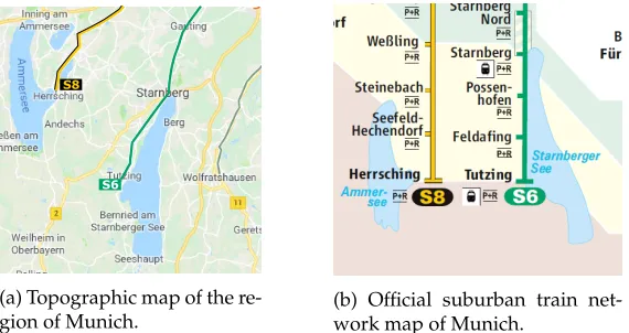
(a) Topographic map of the re-gion of Munich.
(b) Official suburban train net-work map of Munich.
Figure 1: Example of polygonal landmarks usage in schematic maps. It indicates that line S8 goes towards the Ammer lake, and the line S6 passes along the Starnberger lake.
The contribution of this work is a method to produce cognitive adequate schematiza-tions of routes with context information such as side streets, point-like landmarks, and
www.josis.org
Please do not cite
ROUTESCHEMATIZATION WITHLANDMARKS 3
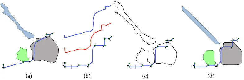
(a) (b) (c) (d)
Figure 2: Schematization process flow. (a) As input, we get the route path, adjacent streets, point-like (black dots) and polygonal landmarks. (b) Original route path in blue (top), rescaled route path in red (middle), and ILP schematization of route path and with ad-jacent streets and point-like landmarks (bottom). (c) Affine transformation to transpose the polygonal landmarks into the schematic route. (d) The polygons are schematized to highlight spatial relations and to fix topological inconsistencies.
mainly, polygonal landmarks. Although some schematic maps designed by cartographers include polygonal landmarks (e.g., Figure 1b), to our best knowledge, no existing au-tomatic drawing methods have explicitly taken into consideration polygonal landmarks schematization in the context of route maps.
Formally speaking, our schematization method takes as its input the target routeRas a geometrically embedded path and adjacent roads represented as stubs. Moreover, the spatial context ofR is given as a set of point-like and polygonal landmarks. The goal is to compute a topologically correct schematic representation of the routeRand its context, which satisfies a number of hard constraints and optimizes an aesthetic quality measure. We implement our approach as a combination of integer linear programming (ILP) for map schematization and local geometric transformations. Figure 2 illustrates the different steps of our method.
In order to evaluate our method, we asked participants to follow textual route descrip-tions together with two map layouts, one with the original shape and another with the schematic layout generated by our algorithm. In 82.8% of the evaluations, participants reported that following the route descriptions was easier with the schematic maps.
The remainder of this article is structured as follows: In Section 2 we review related work on map schematization with emphasis in routes and polygons. In Section 3 we de-scribe the schematization method which includes pre-processing steps (Sections 3.2, 3.1 and 3.3 ), the ILP model (Section 3.4), and the specificities of the route and polygonal landmark schematization (Sections 3.5 and 3.7 respectively). In Section 4 we present the results of our drawing method as well as the results of the user study on the readability of the maps. Contribution, limitations and future work are discussed in Section 5. We conclude our work in Section 6.
JOSIS, Number N (YYYY), pp. xx–yy
Please do not cite
4 GALVAO˜ , KRUKAR, N ¨OLLENBURG, SCHWERING
2
Related work
We divide the related work section into three topics. First, in Section 2.1 we review the bibliography on conceptual models and layout criteria for route maps as an informative tool for wayfinding and spatial learning. Second, in Section 2.2, we review publications on automatic schematization of routes and polygons. Finally, in Section 2.3, we specifically re-view publications that use ILP for schematic map drawing, since ILP is the core technology used in our method.
2.1
Route schematization layout criteria for wayfinding and spatial
learning
Schematic cartography is the application of generalizations to improve a map’s function-ality that goes beyond the adaptation of the map’s features into a specific map scale, i.e., independent of the scale the map is presented at, a generalization is applied because it improves the map’s function as a task solving tool. The cognitive adequacy and the us-ability related to the map’s functionality justifies the schematic layout criteria that are later transformed into drawing rules.
According to Klippel [14], adequate characterization of routes as a visual wayfind-ing tool must emphasize its primitive elements that are mentally conceptualized as route knowledge. Klippel named these primitives wayfinding choremes, and divided them as choremes for turn directions at decision points and choremes for spatial chunking. For turn directions, Klippel proposed seven choremes (SHARP RIGHT, RIGHT, HALF RIGHT, STRAIGHT, HALF LEFT, LEFT, and SHARP LEFT) as a natural human conceptualization of directions and adequate for schematic layout criteria for route knowledge acquisition. Spatial chunking is a combination of two or more elementary route instructions into a single one. For the spatial chunking of routes, Klippel proposed three kinds: numerical chunking that usually makes use of streets adjacent to the route, e.g., “turn left at the third intersection”; structural chunking that uses the structure of the network, e.g., “ at the roundabout, take right”; and landmark chunking, e.g., “ turn left after the gas station”. Chunking route instructions is a natural efficient way to mentally store and communicate route knowledge [13], and therefore, an adequate route schematization must facilitate the readability of features that support spatial chunking.
An adequated representation of turn directions and elements for route chunking is a minimal requirement for a route map as a wayfinding tool [22], however, the literature sug-gests that complementary information, not directly related to route knowledge enrich route maps and promote orientation [18]. Anacta et al. [2] revealed that people make use of local and global landmarks (even if not visible from the route) in maps in order to structure a mental map of the region and orient themselves. Löwen et al. [21] showed that highlighting global landmarks (point-like or polygonal) in assisted navigation devices promotes survey knowledge acquisition. Wiener and Mallot [37] also showed that human route planning takes regions and their spatial relations into account. Schmid et al. [30] highlighted the rel-evance of presenting selected regions and polygonal landmarks in route maps to support structured spatial learning and orientation.
Although the relevance of global and polygonal landmarks in route maps is well ac-cepted, there are no established layout criteria for their schematization in the literature. From public metro map examples, we note that the general principles of schematization to
www.josis.org
Please do not cite
ROUTESCHEMATIZATION WITHLANDMARKS 5
remove unnecessary information (shape, angle, and length generalizations) are applied to polygonal landmarks. Moreover, path-polygon relations used in natural languages [16] are emphasized. Figure 1 exemplifies how a relation “along” is more evident in the schematic layout. Although the Line 6 is not running precisely parallel to the Starnberger lake and in some places the distance between them is over 1km, in the schematic layout the west side of the lake and the train line are collinear.
Another layout criteria frequently applied in route maps is the scale variation, i.e., when different scales are applied to the same map. As pointed out by Delling et al. [6], the in-formation density in a route varies along its path, for example, inside an urban area the number of decision points tends to be much larger than in a highway, and the proper scale to visualize a route depends of this complexity. Schematic cartography allows the application of different scale levels in different parts of a map within a single visualization, what could mitigate the fragmentation of spatial information caused by constant zooming and panning [29]. InThe bounds of distortion[8], Godfrey and Mackaness discuss different kinds of scale variation applied in cartography; they also highlight the relevance of such distortions for the efficacy of navigational information in the context of small devices.
2.2
Route and polygon schematization methods
Although automatic generalization has been an important topic since the beginning of digi-tal cartography, research on automatic schematization started only in the late ’90s and since then has been a prolific topic. The most recognizable example of a schematic map layout is the Tube Map of London’s metro system. Almost all cities that have a metro system also provide their users with a schematic map of the network. For this reason, most of the research on schematization algorithms focused on transit networks [3, 7, 9, 20, 27, 35, 38]. Those methods were surveyed in [25].
In the category ofroute schematization, Agrawala and Stolte [1] proposed a method to schematize routes inspired by handmade route sketch maps. First, short roads are ex-tended to a minimal length to make them more visible. Second, the route path is simplified in a simulated annealing process. Topological inconsistencies and incoherence in the turn-ing angles are penalized in the objective function. This approach is only a path schema-tization, context information like crossing-roads and point-like landmarks are placed in a post-processing step just as edge decoration. Polygonal landmarks are not included.
Delling et al. [5] presented a co-orientated (octilinear) route schematization method that preserves the orthogonal order among all vertices. Their 2-step method uses linear pro-gramming to schematize monotone paths in polynomial time. To be applied in any case, the route path is submitted to a heuristic process that decomposes the route into a minimal set of monotone paths that are joined together after the schematization. The method was further extended [6] to be executed in a single step using ILP. By simplifying the route in a pre-processing step, their solution was mostly able to produce results in less than one second. The distortions in final results tend to be very exaggerated because the total edge length is minimized in the objective function. Delling et al. did not consider landmarks at all.
Polygon schematization gained attention more recently. Buchin et al. [4] presented a quadratic time schematization method for polygons or polygonal subdivisions. Their method iteratively reduces the complexity of the shapes by aligning edges to remove bends. In order to preserve area, a second alignment is selected to compensate the loss or gain
JOSIS, Number N (YYYY), pp. xx–yy
Please do not cite
6 GALVAO˜ , KRUKAR, N ¨OLLENBURG, SCHWERING
of the area. Van Dijk et al. [34] presented a curvilinear polygon schematization method. The algorithms iteratively substitute a pair of adjacent edges for a single circular arc with minimal Fréchet-distance. A substitution is rejected if a topological inconsistency is created or if the distance is out of a given tolerance. Both methods, Buchin et al. [4] and van Dijk et al. [34], show good results for single polygons or polygonal subdivisions, but they were not applied in the context of highlighting spatial relations of regional landmarks in route maps.
2.3
Schematic map drawing with Interger Linear Programming
A schematization method based on Integer Linear Programming (ILP) was first proposed by Nöllenburg and Wolff for the automatic drawing of metro maps [26]. Since then, several publications proposed schematization methods using a similar framework. Oke and Sid-diqui [28] simplified the original model to reduce execution time. Wu et al. [38] extended the model to create space for pictures (annotations) that can be associated with the metro stations. Delling et al. [6], already mentioned in Section 2.2, adapted the model for a path schematization that preserves the orthogonal order of the nodes. Lan et al. [19] extended the model to preserve the representation of major structures of the metro network, e.g., ring lines.
Linear programming is an optimization technique used to find optimal values for real-valued variables that minimize (or maximize) a linear objective function and are subjected to restrictions that must be modeled as linear inequalities. There exist polynomitime al-gorithms to solve linear programming problems. However, some of the constraints require extra variables to represent discrete information, like restricting edge orientations to a fixed set of angles, or to guarantee the correct topology, e.g., a test whether one point is to the left or right of another. Discrete information requires the use of binary or integer variables. Linear programming with integer variables (ILP) is NP-hard, but due to its high relevance in discrete optimization, several practically efficient solvers exist.
For map schematization, the desired variable values are, for example, point coordinates; the hard layout constraints are the restrictions; and soft layout constraints form the objec-tive function as a weighted linear equation that is minimized in the optimization process. For instance, Nöllenburg and Wolff’s model [27] has three soft layout constraints that are minimized together in a weighted objective function: bends, relative positions, and total length:
Minimize αS1costS1+αS2costS2+αS3costS3 (1)
Where costSiis the cost of a soft constraint andαSithe weight of the soft constraint defined
as a parameter.
An ILP-based approach has an important advantage over other methods because the schematization is not limited to a locally optimal solution like in hill-climbing [32] or sim-ulated annealing methods [1, 3], but rather the whole solution space can be inspected to find the solution that exactly minimizes the soft layout constraints. Moreover, topological correctness can be guaranteed as a hard constraint, unlike some other optimizations that in-clude violations in the topology as a cost in the objective function [1]. Specifically, the min-imal edge spacing constraint (preserves planarity), and the circular order constraint (pre-serves the embedding) guarantee a solution with the correct network topology. Notwith-standing, the ILP solution has limitations. First, it is its NP-hardness, which means that too large instances make it impractical, especially for a real-time application. Second,
re-www.josis.org
Please do not cite
ROUTESCHEMATIZATION WITHLANDMARKS 7
stricted linearity is mandatory, i.e., the orientations of the edges are limited to a fixed set of angles. The original approach [26] is octilinear (8 directions), but Nickel and Nöllen-burg [24] demonstrated how to extend the model to be applicable with2kdirections for any integerk.
The major difference in the conceptual model between our method and previous ILP models for schematization [6, 27] is that we do not minimize the total edge lengths in the objective function. This constraint results in a very compact layout adequate for metro maps; however, the scale variation tends to be extreme, causing a distortion that is not always desired for route maps in a driving situation. In our approach, we limit the scale variation level with a parameter in a process before the ILP schematization (Section 3.3). Another important difference is that, instead of running a single ILP model for the whole instance, we run several ILP optimizations for different parts of the instance. As a result, we do not obtain a globally optimal solution for the whole instance, but in compensation, there are some advantages of our approach. First, there is a considerable reduction in the total runtime because of the NP-hardness of the problem. Second, partial results can be delivered while other parts of the instances are processed. And third, distinct ILP models or weights in the objective function can be applied to the different parts of the instance. For example, we use distinct ILP models for the route and for polygonal landmarks.
3
Schematization Method
Start
1.PRE-PROCESSING a) planatization of polygonal landmarks(LM)
b) creation of control edges(CE) c) graph decomposition d) route rescaling transformation
output:
Route path + Stubs + Local point-like LM CE Rescaled route geometry
output: Polygonal LM paths
2.ROUTE + POINT-LIKE LM SCHEMATIZATION
output: Schematized route
4.POLYGONAL-LM PATH SCHEMATIZATION
3.POLYGONAL LM PATH TRANSPOSITION a) adjustment of CE lengths
b) linear transformation
output: Schematized polygonal paths Smooth geometry
End
output: Transposed polygonal LM paths
Sections 3.1 & 3.2
Sections 3.4 & 3.5 Section 3.3
Sections 3.4 & 3.7 Section 3.6
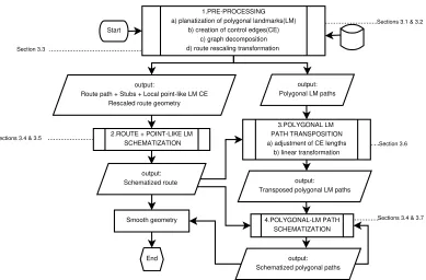
Figure 3: Schematization method flowchart.
JOSIS, Number N (YYYY), pp. xx–yy
Please do not cite
8 GALVAO˜ , KRUKAR, N ¨OLLENBURG, SCHWERING
The flowchart in Figure 3 illustrates the main steps involved in our algorithm. The route data is loaded from a street network database that allows routing algorithms. This street network contains only the topological information, meaning that parallel segments of the same street are collapsed into a single one, the roundabouts were collapsed into a single node, and street links, such as highway exits, were removed.
The process box 1 contains pprocessing steps that prepare the data structures re-quired for the schematization. It gets as input, in addition to the route path, surrounding streets, point-like landmarks, and polygonal landmarks. First, we planarize the polygons with the route. Second, we create special edges (control edges) to connect the point-like landmarks and the disconnected polygonal landmarks to the route; this step is explained in detail in Sections 3.1 and 3.2. Third, we decompose the graph into paths, separating the route, street edges adjacent to the route (stubs), and polygonal landmark paths. Finally, we apply our route rescaling transformation that will define the scale variation on the final map; we explain this step in Section 3.3.
The process box 2 shows the route schematization using ILP. It gets as input the route path, the adjacent streets, and the control edges of the local point-like landmarks. The ILP model uses the rescaled route geometry as a reference for the node positions and proportion of the edges. The output is the schematized route, with the adjacent streets and the point-like landmarks. We describe the ILP model constraints in Section 3.4, and how they are applied for the route schematization in Section 3.5.
The process box 3 contains the steps required before the schematization of the polygonal landmark paths. First, we adjust the length of the control edges to make it adequate to the scale variation of the schematized route. As explained in Section 3.6, the new length of the control edges depends on the length of the edges of the schematized route. Second, we transpose the polygonal landmark paths to the schematized route; for that, we apply a linear transformation that uses the crossing nodes or the control edges nodes as control points.
The process box 4 shows the schematization of the polygonal landmark paths using ILP. It gets as input the transposed paths that are here sequentially schematized. The schema-tized route and previously schemaschema-tized paths need to be submitted to the process in or-der to guarantee the correct topology. The polygonal landmarks ILP schematization is ex-plained in Section 3.7. Finally, for aesthetics reasons, we submit the resulting schematized path (and the route) to a smoothing generalization.
3.1
Control edges for point-like landmarks
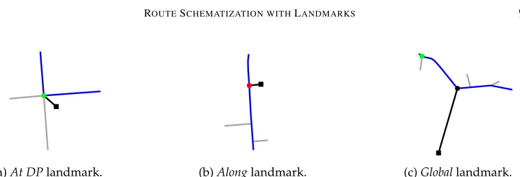
A control edge is a distinct edge created in a pre-processing step (process box 1 in Figure 3) that is used to preserve the relative position of the landmarks with the route. The point-like landmarks are initially loaded as disconnected from the route, so we use control edges to connect them. The way we create the control edges depends on the type of the landmark. We classify the point-like landmarks into types proposed by Löwen et al. [21]: landmarks at decision points (DPs), landmarks along the route, and global landmarks.
For landmarks at DPs, we create an edge connecting the landmark to the DP node (Fig-ure 4a). For landmarks along the route, i.e., close to the route but not at a DP, we add to the route path an extra node at the closest point to the landmark and create an edge connecting this node to the landmark (Figure 4b). For global landmarks, we create an edge connecting the landmark to the closest node in the route path (Figure 4c).
www.josis.org
Please do not cite
ROUTESCHEMATIZATION WITHLANDMARKS 9
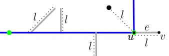
(a)At DPlandmark. (b)Alonglandmark. (c)Globallandmark. Figure 4: Examples of control edges (black edges) created for different classes of point-like landmarks (black squares).
The control edges of the landmarks at DPs and along the route are schematized together with the route and treated as an adjacent edge (Section 3.5). This way, their topology con-cerning the route and the adjacent streets will be preserved. As for the global landmarks, their control edges are not considered by the ILP model. They are used to preserve the rel-ative position of the landmarks with respect to the route. So, after the route is schematized, the new position of the global landmarks are calculated based on the length and the inci-dent angle of their respective control edges. The inciinci-dent angle is preserved, but the length needs to be adjusted to be compatible with the rescaled route. This length adjustment is the same as for polygonal landmarks’ control edges and is explained in Section 3.6.
3.2
Control edges for polygonal landmarks
Before the polygonal landmarks are schematized, we use a linear transformation to adjust their position in relation to the schematized route (process box 3 in Figure 3 ). To support this linear transformation with control points, we create control edges that connect the route with the landmarks. The creation of the control edges depends on the type of the polygonal landmark.
Along the Route landmarks
Along the routelandmarks are polygonal landmarks that are not crossed but that lie within a
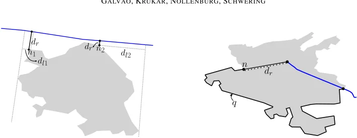
certain distance to the route. For this case, we set a pair of control edges. Figure 5 illustrates the pair of control edges created for a polygonal landmark along the route. The control edge is defined by a control noden(polygon node) and the closest point on the route, where an extra node is created. The control nodes are selected based on two values: the distance to the route (dr); and the distance to the orthogonal line at the beginning (dl1) or end (dl2)
of the linear referencing of the polygon against the route, one for each control edge. The valuesdranddlare weighted in a linear function, and the node with the lowest resulting
value are selected.
Crossed Polygonal landmarks
Crossedlandmarks are polygonal landmarks whose boundaries intersect with the route an
even number of times. They do not need control edges since the crossing nodes suffice as control nodes for a proper adjustment in the affine transformation.
JOSIS, Number N (YYYY), pp. xx–yy
Please do not cite
10 GALVAO˜ , KRUKAR, N ¨OLLENBURG, SCHWERING
dl
1
dl
2
dr d
r
n1 n2
Figure 5: Control edges (black solid line) for polygonal landmarks Along the Route. The control nodesn1andn2are selected because they mutually minimizesdranddl1, anddr
anddl2, respectively.
q
dr
n
Figure 6: A single control edge for
Ori-gin/Destination polygonal landmarks. The
control noden is selected because it mutu-ally minimizes thedrand|q−p/2|.
Origin or Destination Polygonal Landmarks
Originordestinationlandmarks are polygonal landmarks whose boundaries intersect with
the route an odd number of times. Depending on whether the first or the last node of the route is inside the polygon, we classify it as an origin or a destination. One of the crossings is always one control node, therefore only a single control edge is created (Fig. 6). Again, we select the polygon node (n) of the control edges based on two arguments: (1) the distance of the route (dr), and (2) the value specifying how the node, together with the crossing control
node, divide the polygon into two paths of a similar length. Letpbe the perimeter of the polygon, andqthe length of the path connecting the node to the crossing control node. The second argument of the evaluation function is calculated as|q−p/2|.
Global Polygonal Landmarks
Polygonal landmarks are classified asglobalif they are neithercrossednoralong the route, nor theoriginordestination. Polygonal landmarks containing the entire route (e.g., a route inside a city ) are treated asglobal, too. Forglobalpolygonal landmarks, we set a pair of control edges the same way we set it foralonglandmarks. The only difference is a greater weight given to thedl values in a evaluation function. Figure 7 demonstrates how the
control edges are selected if the same landmark is treated asalong(7a), orglobal(7b).
3.3
Route rescaling transformation
The rescaling of the route is a pre-process (process box 1 in Figure 3) of the schematization that creates a scale variation along the route. The Route ILP model uses the rescaled route geometry as a reference for the position of the nodes and the proportion of the edges. The rescaling allocates more space to parts of the route that have a higher concentration of decision points (DPs), making the map more suitable to modern navigation devices with a small screen [8].
Let a DP be a node in the route where a turn is made at a new street, a roundabout, or any salient intersection; we call a path connecting two DPs a route section. The scale of
www.josis.org
Please do not cite
ROUTESCHEMATIZATION WITHLANDMARKS 11
d
l(a) Control edges asAlong the Route.
d
l(b) Control edges asGlobal.
Figure 7: Difference in the creation of control edges if the same landmark is treated asAlong
(a) andGlobal(b). The valuedlforGlobal(b) received a 5 times higher weight in the node
evaluation equation.
s
min
s
k
p
= 0
p
= 0
:
5
p
= 1
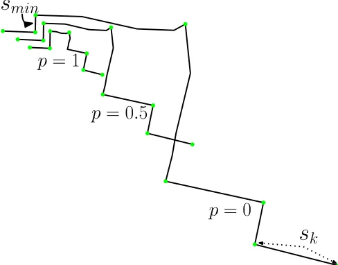
Figure 8: The effect of rescaling of the route using different values forp. In the extreme case (p= 1), all route sections (sub-paths between the green dots) have the length of the shortest route section (smin).
each route section is reduced proportionally to their length using a common parameter that defines the level of distortion. The resulting lengthl(sk)of a route sectionsk is calculated
as
l(sk) =l0(smin) + (l0(sk)−l0(smin))∗(1−pφ(i)) (2)
Wherel0(sk)is the original length ofskandl0(smin)is the given length of the shortest
route section. The float parameterp= [0,1]specifies by how much the sections are reduced.
JOSIS, Number N (YYYY), pp. xx–yy
Please do not cite
12 GALVAO˜ , KRUKAR, N ¨OLLENBURG, SCHWERING
In the minimal distortion (p= 0), the sections keep their original length, and in the maximal distortion (p = 1), the resulting length is the length of the shortest section. We raisepto φ(i) = (l0(smin)
l0(s
k) )
ito increase the effect ofpproportionally to the length of the route sections
(l0(sk)), whereiis a float variable in the range[0,1]. The higher the value ofi, the higher
the effect ofp. All examples present in this paper usei= 0.2.
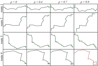
Figure 9: Example of rescaling transformation varying the distortion parameterpapplied to four different routes. Shorter route sections (sub-paths between the green dots) are more visible and the resulting geometry preserve recognizability to the input geometry (p= 0). Route 4 andp= 0.9(in red) is an invalid transformation because violates planarity.
Figure 8 exemplifies the effect of the rescaling transformation in a route path for three differentpvalues: (i) the original route path (p= 0), (ii) an intermediate rescaling distortion (p= 0.5), and (iii) the maximum rescaling distortion (p= 1). Note that, for (p= 1), all route sections get the same length. Moreover, the rescaling transformation shrinks the route geometry, and only the coordinates of the nodes in the shortest route section are preserved. Figures 9 shows the effect of the rescaling process for four different routes and four differentpvalues (p= 0is the original geometry). For each route, we expand the rescaled geometries to have them in a similar extension. Note that the rescaling process allows shorter route sections to be more visible, and at the same time, the resulting geometry maintains similarity to the original geometry. The rescaled route geometry is used as an input in the ILP model that tries to preserve the proportion of its route sections (process box 2 in Figure 3).
www.josis.org
Please do not cite
ROUTESCHEMATIZATION WITHLANDMARKS 13
It is important to mention that the rescaling process is not a topologically safe transfor-mation for non-monotone paths. For example, route 4 andp= 0.9in Figure 9 (red path) contains a violation of the planarity. Some routes have a limit forpuntil planarity is vio-lated; for route 4 in Figure 9, this limit is 0.86. Nevertheless, the rescaling process, in the distortion limit (p= 1), did not violate planarity for more than 95% of the routes we tested. This is because single destination routes generated by shortest path algorithms have a high level of monotonicity.
3.4
The ILP constraints
This section describes the ILP constraints used for the route and for the polygonal landmark paths schematization (process boxes 2 and 4 in Figure 3 respectively). In Sections 3.5 and 3.7 we explain how we apply the constraints for each case.
An ILP schematization process gets as input a graphG= (V, E), whereV is the set of nodes, each of which hasxandyCartesian coordinates, represented here asx(v)andy(v)
for allv ∈V;E is the set of edgese =uvcomposed by a pair of distinct nodes, whereu andv ∈V and where there is a direct link betweenuandv. The expected output are the schematized coordinatesx(v)andy(v)for allv ∈V, such that the layout hard constraints are satisfied and the layout soft constraints are optimized.
The hard constraints areoctilinearity,best turn at DP,stub length,circular order, and
pla-narity. The last two guarantee the topologically correct output. The soft constraints are
bend minimization,edge orientation,node position, androute sections proportion. Some of
con-straints are modeled identically as those used in the original ILP model for metro map [27], others were newly implemented to address the particularity of route maps.
Hard constraint: Octilinearity
Octilinearity is a common rule for metro maps. For route maps, it makes intersection rep-resentations compatible with the 8-directional model of Klippel’s wayfinding choreme the-ory [14]. According to Klippel, a lower level in the granularity of intersections’ angles better reflects a cognitive conceptualization of directions, facilitating their interpretation. Moreover, octilinearity makes crossings of the route with polygonal landmarks more ex-plicit. We modeled this constraint identically to the metro map model [27], nevertheless, an overview of the implementation is necessary to understand the implementation of further constraints.
To guarantee that all edges get an octilinear direction (0◦,45◦,90◦,135◦,180◦,225◦,270◦,
315◦), we define, for each edgee∈E, a supplementary integer variable dir(e)in the range
{0, ..,7}. Figure 10 shows how the eightdirvalues are associated with the octilinear direc-tions. The variable dir(uv)constraints the coordinates ofuandvto force their alignment in the correct octilinear angle. For example, if dir(uv) = 0, i.e, the direction angle ofuvis0◦, the following must hold:
y(u) =y(v) and x(v)> x(u) (3) The dir(e)constraints for other orthogonal directions (0◦, 90◦,180◦ and270◦) can be straightforwardly defined in a similar way as in equations 3. However, for the diagonal directions (45◦,135◦,225◦and315◦), it would require trigonometric functions that are not linear and therefore cannot be used in ILP. To overcome this problem, two new redundant
JOSIS, Number N (YYYY), pp. xx–yy
Please do not cite
14 GALVAO˜ , KRUKAR, N ¨OLLENBURG, SCHWERING
0
j
0
◦1
j
45
◦2
j
90
◦7
j
315
◦3
j
135
◦4
j
180
◦5
j
225
◦6
j
270
◦u
v
Figure 10: Octilinear edge directions. The variable dir(uv)defines the direction ofuv. In this example dir(uv) = 1.
x
z
1y
z
2 22 v
Figure 11: Octilinear coordinate system. If x(v) = 2andy(v) = 2, then, by Equation 4, z1(v) = 2andz2(v) = 0.
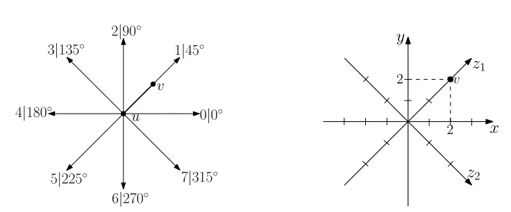
axes, in addition to thexandyaxis, are defined in the coordinate system to represent the diagonals,z1andz2(Figure 11).
For allv∈V, we constrainz1(v)andz2(v)as a function ofx(v)andy(v):
z1(v) =
x(v) +y(v)
2 and z2(v) =
x(v)−y(v)
2 (4)
Now, using thez1andz2 coordinates, we can constrain dir(uv)for the diagonal cases.
For example, if dir(uv) = 1, i.e, the direction angle ofuvis45◦, the following must hold:
z2(u) =z2(v) and z1(v)> z1(u) (5)
It is important to mention that dir(uv)also restricts dir(vu)to its inverse angle. For example, if dir(uv) = 1, then dir(vu) = 5. Figure 10 illustrate this example.
Finally, additional binary variables are necessary to model the case conditions statement that defines the direction of dir(e). Since dir(e)can assume eight directions, eight binary variables would be necessary for each edge; however, to reduce the number of binary vari-ables, we allowdirto assume only one of the three octilinear directions that approximate most to the original orientation.
Hard constraint: Best turn representation at DPs
This constraint forces the turn’s representations into the seven wayfinding choremes. For that, we constrain the direction of the route edges incident on DP nodes to the direction that best represents the original turn. So for each edgeeincident on DP, we set dir(e)to the octilinear direction that best suits the original slope ofuv. For example, if the slope ofeis
40◦, we constrain dir(e) = 1because this is the octilinear direction that best approximates to40◦. To avoid the infeasibility of the model (when a solution cannot be found), we always make sure that there are at least two nodes between DPs.
It is worth noting that there are other ways to model the constraints forbest turns
rep-resentation. For instance, instead of edges’ slope, we could constrain the angle between the
edges incidents on the same DP. Inspired by the wayfinding choremes, we implemented
www.josis.org
Please do not cite
ROUTESCHEMATIZATION WITHLANDMARKS 15
STRAIGHT
VEER RIGHT
RIGHT
SHARP RIGHT SHARP LEFT
LEFT VEER LEFT
(a) Turn directions based on the angle.
STRAIGHT
VEER RIGHT
RIGHT
SHARP RIGHT SHARP LEFT
LEFT VEER LEFT
(b) Klippel et al.’s alternative for turn direction.
Figure 12: Klippel et al. proposed direction models alternatives for route maps [11]. Edge direction at turns can be defined by the region where the original bend lies.
several turn representation based on angles. In Figure 12, we see two alternatives to model octilinear turn directions based on the angle; notwithstanding, we observed consistently better results using the slope of the incident edges. All results presented in this paper use the edges’ slope to model turns at DPs.
Hard constraint: Circular order
Thiscircular orderhard constraint is applied to all degree-3 or higher nodes (more than two
neighbors). It preserves the circular order of the incident edges (embedding). Figure 13 illustrates a degree-knodevand its neighbours:{u1, u2, u3, .., uk}. For a topologically
cor-rect output, the circular order (indicated by the dashed line with an arrow) of the incident edges invmust be the same as the input.
v
uk
u1
u2
u3 u2
Figure 13: The circular order of the incident edges in an node must be preserved
In order to guarantee the circular order of the incident edges inv, we need to constrain dir(e)for alleincident tovas follows:
dir(vui+1)≥dir(vui) + 1 (6)
An exception is necessary for the last and the first edge relation (dir(vuk)and dir(vu1)).
We ommit details here, because this constraint is modeled identically to the metro map model (See [27, Section 3.2] for details).
JOSIS, Number N (YYYY), pp. xx–yy
Please do not cite
16 GALVAO˜ , KRUKAR, N ¨OLLENBURG, SCHWERING
Hard constraint: Planarity
Theplanarityhard constraint prevents pairs of non-incident edges from touching or
cross-ing themselves (preserve planarity). Together with thecircular orderconstraint,planarity
guarantees a topologically correct schematization. We explain only the principle behind the modeling of the inequalities because it is modeled identically to the metro map model. (See [27, Section 3.3] for details).
v2 v1 u1
u2
e1
e2
Figure 14: The conjunctive expression 7 holds true fore1ande2, soe2is completely south
frome1.
Figure 14 shows two distinct edges,e1ande2, and their respective nodes. To facilitate
the explanation, let the octilinear directions be cardinal directions:0◦is east,45◦ is
north-east,90◦is north,135◦is northwest, and so on. To say thate2is completely south frome1,
the following conjunction of inequalities must hold:
y(u2)< y(u1) ∧ y(u2)< y(v1) ∧ y(v2)< y(u1) ∧ y(v2)< y(u2) (7)
If we constrain e2 to be completely south from e1, we guarantee that e2 and e1 are
not crossing. Analogous conjunctive expressions can be defined for all other 7 octilinear cardinal directions using thex,y,z1, andz2 coordinates. Therefore, to guarantee thate1
ande2do not cross themselves, at least one of eight conjunctive expressions must be true.
Hard constraint: Edge length
Theedge length hard constraint is used to guarantee that all side streets edges have the
same length or that all local point-like landmarks are equally spaced from the route. The constraint to fix the length of an edgeedepends on the direction ofe, i.e., dir(e). We present the case for dir(e) = 0like illustrated in Figure 15. The constraints for other directions are modeled analogously.
l
l
l
l
u
v
u
l
e
Figure 15: Hard constraintedge lengthfixes the lengths of the side streets (in gray) and local point-like landmarks (large black dot) control edges to a given valuel.
Recall Equation 3 with the constraints to guarantee dir(uv) = 0 (and the analogous constraints for other directions). We modify this constraint by adding a parameterl that
www.josis.org
Please do not cite
ROUTESCHEMATIZATION WITHLANDMARKS 17
represents the desired length ofuv, and by change the inequalitygreater thantoequal toas follows:
y(u) =y(v) and x(v) =x(u) +l (8)
Soft constraint: Node position
We use thenode positionsoft constraint to minimize the distance of the output coordinates to the input coordinates of the nodes. They are applied to the route (rescaled coordinates) and to the polygonal landmarks (transposed path). Thenode positionsoft constraint improves coherence in the relative position among all nodes, i.e., it contributes for topographicity. This constraint is not present in the original metro map model; therefore, we describe its implementation in detail. The general idea is to add a cost in the objective function propor-tional to the distance of the input and output coordinates for each node.
The cost of thenodes positionto be minimized in the objective function is:
X
(dx(v) +dy(v)) ∀v∈V (9)
wheredx(v) = |x(v)−x0(v)|anddy(v) = |y(v)−y0(v)|. Note that we use Manhattan
distance instead of Euclidean distance because square roots are not linear functions and therefore cannot be used in an ILP model.
We can divide our cost function into two terms, one for thex-coordinates and another for they-coordinates and minimize them individually:
X
dx(v) + X
dy(v) ∀v∈V (10)
An absolute value operator inside an ILP model usually requires the use of a binary variable in order to treat the positive and the negative cases differently. However, an abso-lute value operation can be modeled using two inequalities if it is an increasing function in-side an objective function to be minimized. We show the inequalities for thex-coordinates. They-coordinates are modeled analogously:
dx(v)≥ x0(v)−x(v) (11a)
dx(v)≥ −(x0(v)−x(v)) (11b)
Soft constraint: Proportion
Theproportionsoft constraint is used to minimize the difference between edge lengths in the
input and output. It improves distance coherence between adjacent nodes. We also model this constraint to maintain proportionality of route section lengths, i.e., to reduce length distortions between decision points. Thenode positionconstraint already contributes to this proportionality, but it is not always sufficient to guarantee a balanced result in terms of route section lengths. Figure 16 contrasts a schematizationwithouttheproportionconstraint for route sections with onewiththe proportion constraint for route sections.
Theproportionconstraint is not present in the original metro map model [27].
There-fore we describe it in detail here. For simplicity, we explain the constraint to keep length proportionality of all edges. Notwithstanding, the same principles can be applied to route sections; for that, consider only the DP nodes instead of all nodes.
JOSIS, Number N (YYYY), pp. xx–yy
Please do not cite
18 GALVAO˜ , KRUKAR, N ¨OLLENBURG, SCHWERING
(a) Original route path. (b) Schematization without pro-portion constraint.
(c) Schematization with propor-tion constraint.
Figure 16: The effect of theproportionconstraint for route sections.
For each edgeuv∈E, we define a variable∆p(uv)that expresses the difference of the resulting edge length and the input edge length as
∆p(uv) =|l0(uv)−l(uv)|, (12)
wherel0(uv)is the original edge length ofuv, and the variablel(uv)denotes the result-ing edge length
l(uv) = (|x(v)−x(u)|+|y(v)−y(u)|). (13) This time we have two absolute value operations to describe a variable in our ILP model. In this case, we need, for each of them, a pair of binary variables to model the absolute value operation in a case system of linear equations. We show our model for the x-coordinates. They-coordinates are analogously modeled.
Letdx(uv) =|x(v)−x(u)|be the absolute value function, thendx(uv)can be expressed
as
dx(uv) = (
x(v)−x(u) ifx(v)≥x(u)
x(u)−x(v) ifx(u)≥x(v). (14) To model this case distinction system in our ILP model we define for each edge a pair of binary variablesλx1(uv)andλx2(uv)and constrain them as
λx1(uv) +λx2(uv) = 1. (15)
Now we can define the following inequalities
dx(uv)≤(x(v)−x(u)) +M(1−λx1) (16a)
dx(uv)≥(x(v)−x(u))−M(1−λx1) (16b)
dx(uv)≥ −(x(v)−x(u))−M(1−λx2) (16c)
dx(uv)≤ −(x(v)−x(u)) +M(1−λx2). (16d)
Note that ifλx1(uv) = 1, by Equations 16a and 16b, we getdx(uv) = (x(v)−x(u)), and
Equations 16c and 16d are trivially fulfilled (obsolete) becauseMis a large enough constant. Analogously, ifλx2(uv) = 1, by Equations 16c and 16d we getdx(uv) = (x(u)−x(v)), and
Equations 16a and 16b are trivially fulfilled (obsolete). Now, we can express
∆p(uv) =|l0(uv)−(dx(uv)−dy(uv))|. (17)
www.josis.org
Please do not cite
ROUTESCHEMATIZATION WITHLANDMARKS 19
Again we have an absolute value operation inside an objective function to be mini-mized. Similarly to Equation 11, we use two constraints to model Equation 17.
∆p(uv)≥l0(uv)−dx(uv) +dy(uv) (18a) ∆p(uv)≥ −l0(uv) +dx(uv)−dy(uv). (18b)
Soft constraint: Bend minimization
Thebend minimizationsoft constraint reduces the number of bends along the route. It
di-minishes unnecessary complexity along the route path in order to facilitate path following by the user. For polygonal landmarks, it contributes to increasing abstraction. We model this constraint in the same way it is modeled to reduce bends along the transit lines in the metro map model [27]. For this reason, we only give an overview of its implementation (See [27, Section 3.5] for details).
LetP be a path (the route path or a polygonal landmark path) andvba degree-2 node
inP. The cost of thebend minimizationin the objective function is:
X
b(vb) ∀vb∈P, (19)
whereb(vb)represents the individual cost of the bend formed by the incident edges in
vb, and is calculated as
b(vb) = (
|dir(u1vb)−dir(vbu2)| if |dir(u1vb)−dir(vbu2)| ≤4
8− |dir(u1vb)−dir(vbu2)| if |dir(u1vb)−dir(vbu2)| ≥5.
(20)
Let u1 and u2 be the two nodes adjacent to vb, as exemplified in Figure 17. In this
example we have dir(u1vb) = 0and dir(vbu2) = 5, so|dir(u1vb)−dir(vbu2)|= 5; then, by
Equation 20,b(vb) = 3. Equation 20 has the property to give higher costs to acute bend
angles compared to obtuse ones: 0 for0◦, 1 for135◦, 2 for90◦, and 3 for45◦.
v
bu
1
u
2
Figure 17: The bend angle formed by edgesu1vbandvbu2is45◦. By Equation 20, the cost
of this bend (b(vb)) is 3.
Soft constraint: Edge orientation
The soft constraintedge orientation is used to minimize the difference of edges’ direction between the input and output. This constraint counterbalances potential undesired distor-tion caused by thebend minimizationconstraint. For the route path, it improves the sense of direction along the route path, and, for the polygonal landmark paths, it contributes to a more genuine shape (less abstract). We modeled this constraint identically to the edge
directionconstraint in the metro map model [27, Section 3.6].
Let(e)be a binary variable constrained as
8(e)≤dir(e)−dir0(e)≤8(e) ∀e∈E, (21)
JOSIS, Number N (YYYY), pp. xx–yy
Please do not cite
20 GALVAO˜ , KRUKAR, N ¨OLLENBURG, SCHWERING
where dir0(e)is the octilinear direction angle ofe that approximates best its original slope. For instance, if the slope angle ofeis40◦, then dir0(e) = 1. Because|dir(e)−dir0(e)|< 8, by Equation 21,(e) = 0if and only if dir(e) =dir0(e), otherwise(e) = 1.
The cost of theedges orientationin the objective function is:
X
(e) ∀e∈E. (22)
3.5
Route and point-like landmarks schematization
The ILP model for the route and point-like landmarks schematization gets as input the route path, its adjacent streets, and the control edges of the local point-like landmarks. In order to reduce the size of the instance, we simplify the route path using the Douglas-and-Peucker simplification method to remove some degree-2 nodes. We use a sufficiently low enough tolerance in the simplification to keep the topographicity of curves along the route. Moreover, we guarantee that at least two nodes remain between intersections (degree-3 or higher nodes). Keeping these two nodes improves the final representation of intersections and guarantees the feasibility of ILP in respect to thebest turns at DPhard constraint. After the ILP execution, we reinsert the removed nodes into the route path because we want to retain the geographic coordinates associated with them.
ILP model hard constraints areplanarity,circular order,octilinearity,best turn at DP, and
edge length. Theedge lengthfixes the lengths of the adjacent street edges and the local
point-like landmark control edges to a fixed value. The longer the edges, the higher the chances of planarity violations, which potentially increases the execution time. Thecircular order
and planarityconstraints guarantee topologically correct results. However, theplanarity
constraint represents to the whole model 32 constraints and eight binary variables for each pair of non-incident edges. Since the number of non-incident edges pairs is roughlym2/2,
wheremis the total number of edges, planarity is the most costly constraint of the model. In order to reduce the runtime of our application, we implement this constraint in a “lazy” way as used by Delling et al [6]. First, the instance is schematized without theplanarity
constraint, and, while the output contains edge crossings, we rerun the ILP only including in theplanarityconstraint for pairs of edges that crossed in the previous executions.
There are five soft constraints in the ILP model:node position(dist),edge orientation(dir),
bend minimization(bend),proportionfor route edges (prop), andproportionfor route sections
between DPs (propDP). The objective function is defined as follow:
Minimize α1
ncostdist+ α2
mcostdir+ α3
b costbend+ α4
mcostprop+ α5
s costpropDP (23) Theαi values are parameters to weight the cost of each soft constraint. The variables
n,m,b, andsare the number of nodes, edges, bends (degree-2 or higher nodes), and route sections, respectively; they normalize the given weights. Note that we use theproportion
constraint twice. One is used to keep the length coherency of all edges, and the other applied only for the route sections.
Figure 18 demonstrates the results of the route schematization with point-like land-marks (black dots). Note that in the schematized layout (Figure 18b), landland-marks along the route are evenly spaced away from the route, creating enough space to replace the point geometries with icons, as shown in Figure 18c.
www.josis.org
Please do not cite
ROUTESCHEMATIZATION WITHLANDMARKS 21
(a) Original layout (b) Schematized layout (c) Dots replaced by icons
Figure 18: Example of a route schematized with point-like landmarks
3.6
Path Transposition: Adjustment of Control Edges’ Lengths
The control edges are used to preserve the relative positions of the polygons to the route. After the route is schematized, we use linear transformation to transpose the polygonal landmark paths to the schematized route using the nodes of the control edges as control points (process box 3 in Figure 3). However, because of the rescaling of the route, we need to rescale the control edges too. The scale along the schematized route varies from section to section, meaning that the scale factor cannot be the same for all control edges. For a coherent rescaling, we adjust the length of the control edges based on the length of the schematized route edges. LetErbe the set of route edges, andl0(er)andl(er)the lengths
of the original and schematized route edgeer ∈ Er, respectively. The ratio of the new
length for each control edge is calculated as:
Xl(er)
d(er)
/Xl 0(e
r)
d(er)
∀er∈Er and d(er)<0.8, (24)
where d(er)is the normalized (scaling[0,1]) distance of the route edge er to the control
edge. Because we weight each route edge by the inverse of its distance to the control edge, route edges closer to the control edges will have a higher influence on the resulting length of the control edge. Moreover, we ignore route edges that are too far away from the control edge (d(er)≥0.8).
3.7
Polygonal landmark path schematization
The ILP for polygonal landmark paths schematization gets as main input the transposed geometries of the polygons obtained from a linear transformation. The linear transfor-mation uses crossing nodes or the control edges nodes as control points (process box 3 in Figure 3). Figure 19b illustrates the transposed paths (black lines) as a result of this process. Before we run the ILP and similar to preprocessing the route, we use a Douglas-Peucker simplification to reduce the number of nodes, and, consequently, the ILP run time. The simplification tolerance must be limited in order to preserve the general morphology of
JOSIS, Number N (YYYY), pp. xx–yy
Please do not cite
22 GALVAO˜ , KRUKAR, N ¨OLLENBURG, SCHWERING
(a)
(b) (c)
Figure 19: Polygon schematization workflow: (a) Before the route is schematized we create control nodes (yellow dots) and control edges (red lines) for each polygon. (b) After the route is rescaled and schematized, we adjust the control edges’ length in order to use the control nodes in the affine transformation to transpose the polygons (black outlines). (c) Finally, the transposed polygons are schematized using ILP
the landmarks. We also guarantee that the control nodes are maintained. After the ILP execution, we reinsert the removed nodes into the path.
The ILP model hard constraints for the polygonal landmark path schematization are
octilinearityandplanarity. We use the same iterative planarity check as for the route ILP.
First, the instance is schematized without the planarity constraint, and, while the output contains edge crossings, we rerun the ILP including the planarity constraints for those pairs of edges that crossed in previous executions.
There are five soft constraints in the polygon schematization ILP model: node position
(dist),node positionfor control nodes only (distCN),edge orientation(dir),bend minimization
(bend), andproportion(prop). The objective function is defined as:
Minimize α1
ncostdist+ α2
c costdistCN+ α3
mcostdir+ α4
b costbend+ α5
mcostprop. (25) Theαivalues are the parameters to weight the cost of each soft constraint. The variables
n,m,b, andc are the number of nodes, edges, bends (non degree-1 nodes), and control nodes respectively; they normalize the given weights. Note that we use a second node
positionconstraint only for the control nodes. This way we can discriminate the weight for
thenode positionbetween control nodes and ordinary nodes.
The polygonal landmark ILP schematization is used to meet four goals: (i) reduce the shape complexity (abstraction); (ii) guarantee the correct topology with previously
schema-www.josis.org
Please do not cite
ROUTESCHEMATIZATION WITHLANDMARKS 23
tized features; (iii) emphasize spatial relations (crossings and alongness), and (iv) control the dimension of the landmarks.
Abstraction
Abstraction involves reducing the shape complexity of the map’s features. It is one of the main characteristics of schematic visualizations. Abstraction contributes to a cleaner layout by removing unnecessary information, driving the attention of the user to more functional elements of maps. Nevertheless, abstraction reduces recognizability of landmarks because it leads to severe changes in the original geometry.
We control the level of abstraction by weighting the cost of the soft constraints. The constraintbend minimizationincreases abstraction, and constraintsedge orientationandnode
positionincrease topographicity. Figure 20 illustrates the abstraction’s effect on the
land-mark geometries that results from variations in the soft constraints’ weights.
(a) original (b) lower abstraction - dir 56.1, bend 5.5
(c) medium abstraction - dir 45.1 - bend 30.5 (d) higher abstraction - dir 12.1 - bend 45.5
Figure 20: Balancing the level of abstraction by varying the weights of the soft constraints. The caption values are the weights for theedge orientationandbend minimization(α3andα4
in Equation 25). The weights for the remaining constraints are constant (1580, 790, and 500 forα1,α2, andα5respectively)
The weights for the soft constraints can also be dynamically adjusted. This means that the level of abstraction can depend on attributes of landmarks, such as type, size or distance to the route.
Fixing topological inconsistencies
Merely transposing the polygon using an affine transformation does not guarantee topo-logical consistency with previously schematized features. Figure 21b shows a polygon transposed to a schematized route. Note that the botton-left part of the polygon contains crossings with the route nonexistent in the original layout (Figure 21a). Theplanarity con-straint can prevent such crossings in the resulting layout. For that, we need to input pre-viously schematized edges from the route and other polygonal landmarks into the ILP process (process box 4 in Figure 3).
JOSIS, Number N (YYYY), pp. xx–yy
Please do not cite
24 GALVAO˜ , KRUKAR, N ¨OLLENBURG, SCHWERING
(a) (b) (c) (d)
Figure 21: ILP fixes topological inconsistencies. (a) Original route crosses the polygon shape, (b) The polygon transposed to the schematized route contains extra edge crossings. (c) Octilinear bounding box (dotted line), and detection of edges (red) to avoid crossing. (d) Schematized polygon with correct topology
Every shape schematized in the ILP is bounded by an octilinear box defined by the limit of the octilinear coordinates. This way, it is necessary to check for planarity violations only for the edges intersecting this bounding box region. Figure 21c illustrates the octilinear bounding box (black dotted lines) that limits the position of the path nodes, and the edges of the schematized route (in red) that intersects the bounding box region. The resulting schematization with correct topology is shown in Figure 21d.
Emphasizing spatial relation
Landmarks along the route can be used in spatial chunks (e.g., go along the park and turn left). We can increase alongness (ratio of the region boundary being parallel to a path) with the route by reducing the length of its pair of control edges before transposing the polygon. Figure 22 illustrates the effect of this tighter adjustment. Because we shortened the control edges (little black line segments) in Figure 22c, the polygonal landmark got closer to the route after the transposition of its path. As a result, its schematic layout has a higher degree of parallelism with the route compared to Figure 22b.
(a) original shape. (b) regular. (c) tight.
Figure 22: Emphasizing alongness: the control edges (dashed black lines) for (C) are short-ened.
Scale control
The polygonal landmark ILP schematization can be used to control the size of the land-marks. For example, a landmark along a route section with an enlarged scale can have its size extended beyond the desired limit. Figure 23c illustrate such a case. Note that the
www.josis.org
Please do not cite
ROUTESCHEMATIZATION WITHLANDMARKS 25
parks have their size over-exaggerated compared to the original layout (Figure 23a). This happens because the route sections along the parks have their scale relatively enlarged af-ter the route rescaling transformation, and this has an effect on the scale in the transposed landmark paths (black outline in Figure 23b).
(a) original. (b) transposed paths. (c) no scale control. (d) with scale control.
Figure 23: Effect of scale control.
We can control the size of landmarks using theedge proportionsoft constraint. For that we add a parameterqto the Equation 12:
∆p(uv) =|q∗l0(uv)−l(uv)|. (26)
The parameterqmodifies the resulting length of the edges. Ifqis equal to1the edges lengths will tend to have the same length (l0(uv)) as the respective edges of the input (trans-posed path). We calculateqby, first, estimating the ideal length of the landmark path using the same equation for the adjustment of the control edges (Equation 24 in Section 3.6). Then, the value qis calculated as the ratio of the ideal length over the transposed path length. Figure 23d shows the result of scale control of the landmarks along the route using the parameterq. For instance, the rightmost park,qwas set to0.73, i.e., its edges’ lengths are preferred to be 73% of the respective input edges’ lengths.
The last change to control the scale of a landmark is to remove thenode position con-straint (settingα1= 0in Equation 25). We removenode positionbecause we want to change
the extension of the input path (transposed). So we do not need to minimize the distances of the nodes to the input positions. We keep only thenode positionconstraint for the control nodes (distCN in 25). Then only the control nodes (landmark control edge nodes) will have their distance to the respective input nodes minimized.
4
Results
Figure 24 illustrates a typical result of our schematization method. It shows the input data of a 33.7km long route connecting two cities. The instance submitted to schematization is composed of 317 nodes, of which 172 belong to the route, adjacent streets, and the point-like landmarks, and 145 to the polygonal landmarks. We count here only the number of nodes after the Douglas-Peucker simplification, i.e., the actual size of the instance submitted to ILP process. The total execution time was 6.189 seconds, of which 5.2 seconds for the route, and 0.983 for 8 landmarks. We ran our application using an 8GB RAM Intel Core i7 2.8 GHz Windows 10 Laptop and IBM CPLEXRV12.7.1 to solve the ILP model. Also, for all ILP executions, we set the relative MIP gap tolerance to 0.1, i.e., CPLEX stops the execution as soon as it finds a feasible integer solution proved to be within ten percent of optimal.
JOSIS, Number N (YYYY), pp. xx–yy
Please do not cite
26 GALVAO˜ , KRUKAR, N ¨OLLENBURG, SCHWERING
Figure 24: Example of input and output of our method with annotations.
General
nodes edges rescaled paths poly. LM point LM fixed cross. ILP exec. runtime
317 304 0.77 12 8 13 0 13 6189ms
Route
nodes edges DPs stubs αbend αdir αdist αprop αpropDP ILP exec. runtime
172 171 12 60 100 43.5 43.5 100 200 1 5206ms
Polygonal landmark paths
paths nodes edges αbend αdir αdist* αdistCN αprop ILP exec. runtime
12 145 13 25 52.8 1000 500 500 12 983ms
Table 1: Schematization summary of Figure 24.
Table 1 shows the main information on the instance and the weights used in the objec-tive function. The weights are shown as theαvalues used in the Equation 23 for the route, and in the Equation 25 for the polygonal landmark paths. The 12 polygonal landmark paths are individually schematized but, to be more concise, we summarize their schematization information into a single table. For that we use the same weights in the objective function for all landmarks, except for thenode positionconstraint of the landmarks along the route. For them, the valueαdistis zero because of the scale control explained in Section 3.7.
Yet in Figure 24, we compare the original with the resulting layout in the same space extension. In order to facilitate the description of the schematic layout criteria effects, we added reference annotations (numbers inside circles) to the input figure. Note that, for parts of the route with a higher density of DPs and landmarks, the scale is larger (7), and for parts of the route with fewer elements the scale is smaller (5); that way, short route sections and small polygonal landmarks are more visible in the schematic layout. Unnecessary
www.josis.org
Please do not cite
ROUTESCHEMATIZATION WITHLANDMARKS 27
bends along the route path were removed (3), and important crossings and turns were made more evident (1, 6), in line with the wayfinding choremes theory [14]. The placement of point-like landmarks (black dots) is consistent with the original (8); those that were too close were pushed away from the route, making it easier to identify on which crossing corner or which side of the route they are located. As for the polygonal landmarks, their shape was simplified making them more abstract (4), their crossing with the route became more orthogonal and, for those along the route, the parallelism became more evident (2).
(a) input (b) output
Figure 25: Example of input and output. The route goes along a park (green) and crosses the city center (gray). The lake (blue) is a global landmark. There are seven DPs and three point-like landmarks.
General
nodes edges rescaled paths poly. LM point LM fixed cross. ILP exec. runtime
135 130 0.5 4 4 3 7 10 2281ms
Route
nodes edges DPs stubs αbend αdir αdist αprop αpropDP ILP exec. runtime
78 77 7 15 50 75 75 100 75 1 705ms
Polygonal landmark paths
paths nodes edges αbend αdir αdist* αdistCN αprop ILP exec. runtime
4 57 53 25 48.4 1000 500 500 9 1576ms
Table 2: Schematization summary of Figure 25. Five extras ILP executions were necessary to fix 7 edge crossings that violated the topology.
JOSIS, Number N (YYYY), pp. xx–yy
Please do not cite
28 GALVAO˜ , KRUKAR, N ¨OLLENBURG, SCHWERING
Figure 25 shows a second example of output for a 3.7km route. This instance is com-posed of 135 nodes, of which 78 belong to the route, adjacent streets, and the point-like landmarks, and 57 to the polygonal landmarks. The total execution time was 2.281 sec-onds, of which 0.7 seconds for the route, and 1.58 seconds for 3 polygonal landmarks. Note that in this example 9 ILP executions were required for the 4 polygonal landmark paths (Table 2). The extra ILP executions were necessary to fix edge crossings that violated the topology as identified after the first executions.
4.1
Evaluation
We designed an experiment to evaluate the readability of route information in the result-ing schematic layouts. In this experiment, we presented the participants with a textual route description composed of an ordered list of instructions, and two corresponding map layouts: a topographic version (with the input coordinates), and a schematic version gen-erated by our algorithm. Then, we asked participants to read the instructions and follow them in both maps. Figure 26 illustrates three examples of routes we used in the experi-ment. Afterwards, participants were asked to answer two questions:On which layout is the route instructions easier to follow? Which layout symbolizes better the route instructions?
Participants were asked to repeat this procedure for 19 different routes, where the focus of the maps was divided into three different aspects of the algorithm that we wanted to evaluate: (i) schematization of the route and side streets (Figure 26a), (ii) route and place-ment of the point-like landmarks (Figure 26b), and (iii) spatial relations of the route with the polygonal landmarks (Figure 26c).
Easier to follow Symbolizes better Aspect focus Original Schematic Total Original Schematic Total
Route only 19 143 162 32 130 162
Point-like landmarks 23 112 135 28 107 135
Polygonal landmarks 46 170 216 71 145 216
All routes 88 425 513 131 382 513
Table 3: Evaluation results. Participants layout preference (original vs. schematic) on two questions: On which layout are the route instructions easier to follow? Which layout symbolizes better the route instructions?
We collected data from 27 participants (17 female, 10 male, and an average age of 29,56 years). Most of whom were recruited in social media groups and in a general mailing list of the university students. Each participant responded to 19 routes, resulting in the total of 513 observations. Table 3 shows the results of the evaluation reported by the participants divided by the aspect focus. In total, in 82.8% of the evaluations, participants reported route instructions in the schematic layout to be easier to follow, and 74.5% of the evaluations, participants thought that the schematic layout symbolizes route instructions better.
5
Discussion
Schematic cartography makes use of generalizations to improve specific functionalities of a map. As discussed in the introduction, we are investigating visualizations whose
pri-www.josis.org
Please do not cite
ROUTESCHEMATIZATION WITHLANDMARKS 29
(a) route and side streets.
(b) point-like landmarks.
(c) polygonal landmarks.
Figure 26: Example of routes used in the experiment: in Figure 26a the focus is on the route and side streets only, in Figure 26b the focus is on the point-like landmarks, and in Figure 26c the focus is on the polygonal landmarks.
mary functions are to facilitate the readability of route information and the acquisition of survey knowledge. As presented in the Results section, our route schematization method achieved the layout criteria for a functional route map, i.e., emphasized turns at decision points, crossings, elements for spatial chunking [13], and the route’s spatial relation with contextu
![Figure 12: Klippel et al. proposed direction models alternatives for route maps [11]. Edgedirection at turns can be defined by the region where the original bend lies.](https://thumb-us.123doks.com/thumbv2/123dok_us/1157653.1617867/15.612.264.361.457.550/figure-klippel-proposed-direction-alternatives-edgedirection-dened-original.webp)