Modified Huffman Algorithm for Image Encoding and Decoding

(1)

Modified Huffman Algorithm for Image Encoding and Decoding

Sona Khanna, Suman Kumari

, Tadir

Department of Computer Science and Engineering

, Guru Nanak Dev University RC, Gurdaspur, India

ABSTRACT

Lossless compression of a progression of symbols is a decisive part of data and signal compression. Huffman coding is lossless in nature; it is also generally utilized in lossy compression as the eventual step after decomposition and quantization of a signal. In signal compression, the disintegration and quantization part seldom manages to harvest a progression of completely autonomous symbols. Here we present a schema giving prominent results than forthright Huffman coding by exploiting this fact. We cleft the inceptive symbol sequence into two arrangements in such a way that the symbol statistics are, sanguinely, different for the two possessions. Sole Huffman coding for each of these disposition will reduce the average bit rate. This split is done recursively for each arrangement until the cost league with the split is larger than the attainment. Assay was done on distinct signals. The harvest using the cleft schema was a bit rate devaluation of ordinarily besides than 10% compared to forthright Huffman coding, and 0- 15% surpassing than JPEG-like Huffman coding, inimitable at low bit rates.

Keywords: Lossless Compression, Huffman Coding, Disintegration

I. INTRODUCTION

Huffman coding contrives variable-section codes, each interpreted by an integer number of bits. Symbols with higher anticipation get curtailed codewords. Huffman coding is the best coding schema possible when codewords are restricted to integer section, and it is not too complex to implement [1]. It is therefore the entropy-coding schema of elite in frequent applications. The Huffman code tables usually required to be included in the bunched file as side information. To avoid this one could utilize a standard table derived for the relevant class of data, this is an option in the JPEG compression schema [4]. Another alternative is adaptive Huffman coding as in [3]. While these mechanisms do not need side information they utilize non-optimal codes and consequently besides bits for the symbol codewords. The efficiency of Huffman coding can often be significantly bettered by the utilize of custom made Huffman code tables. This possibility is also included in the JPEG compression schema [4]. The mechanisms utilized in this paper all utilize custom made Huffman code tables. Huffman coding is adequate when integer

codeword sections are advisable for the symbol sequence. Generally, this is the case when no symbols have very high anticipation, especially no symbol should have probability greater than 0.5. If the symbols anticipation are 0.5, 0.25, 0.125, 0.0625 or fewer than 0.05 then a schema using integer codeword sections will do quite well. Huffman codes do not exploit any dependencies between the symbols, so when the symbols are statistically dependent other mechanisms may be much better.

II. METHODS AND MATERIAL

1.1 Lossy Signal Compression

Lossy signal compression often has the following steps 1. Decomposition.

2. Quantization, often with threshold. 3. Run Section and End Of Block coding. 4. Huffman coding.

(2)

man coding. The two first steps are identical for all three mechanisms, we utilize DCT and uniform quantization with threshold. The results can then be interpreted in a matrix where the rows are the frequencies and the columns are time. The entries are the quantized values, there are as frequent entries as there are samples in the signal. The upper left part of this matrix may be

Table 1: Shows the Quantized values of the image

Since we have utilized a 16 points DCT, the matrix will have 16 rows (bands) and each block is 16 samples. The three different mechanisms utilized here all start with this matrix of quantized bits, and utilize different ways to form the symbol arrangement Forthright Huffman Coding utilize only End of Block coding. The End of Block symbol, (0), and the rest of the symbols are formed from the quantized values according to this table

Table 2: Showing End of Block Coding

The symbol sequence after EOB coding for the example above will then be:

9, 3, 0, 11, 1, 3, 0, 11, 7, 3, 0, 0, 8, 1, 1, 11, 0, 4, 2, 9, 0, 9, 1, 3, 0, 5, 4, 1, 2, 0, · · ·.

We note that there will be as frequent EOB symbols as there are columns in the matrix, and that the symbol sequence will be non-negative integers where the petite ones are besides probable than the larger ones, utilize symbols interpreted by small integers correspond to small magnitude of the quantized values.

JPEG-like Huffman Coding makes the symbols the clone way as JPEG does, each column of the matrix correspond to the zigzag scanned sequence of a 8 × 8 pixel picture block in JPEG. The DC component and the

AC components are coded separately. The DC component is DPCM coded and the symbols are illustrate by the following table

Table 3: Showing Structure of the tree through Huffman coding

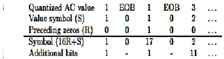
Each symbol is followed by some supplementary bits to uniquely give the DPCM difference. For the data example this gives (the two last lines are stored) For the AC component the zeros are run section coded. Each symbol consists of two parts, the first part is the run that tells how frequent zeros that precede the value (R), and the second part is the value symbol (S). The value symbols are the clone as the symbols utilized for the DPCM differences. To completely specify the value each symbol is succeeded by supplementary bits the clone way as for the DPCM differences. The combined symbol (interpreted as one integer) is 16R + S. Symbol (0) is EOB. For the example data this gives

Table 4: showing the Quantized Values with preceding zeros

(3)

integer codeword sections are not advisable then other mechanisms may be much better.

2. Disband the Symbol Sequence

The basic idea is that by disband a long sequence into several curtailed ones in a way that makes the symbol anticipation (and the optimal code sections) different for each sequence, then individual Huffman coding of each sequence will reduce the total number of bits utilized for the codewords. On the other hand, there will be besides Huffman code tables to include. Clever disband combined with adequate coding of the side information should give an improvement in overall bit rate. We choose to utilize a schema that first splits the symbol sequence after End of Block coding into three arrangements.

2.1. Disband into three Arrangement

When we examine the End of Block coded sequence we make the following observations

• A symbol succeeding an EOB symbol (0) is the DC component, or possibly another EOB symbol. • An EOB symbol (0) will never succeed a (1)

symbol.

This may be exploited by creating three symbol arrangements from the original sequence. The first sequence contains the first symbol and the symbols following a (0) symbol, the next sequence contains the symbols following a (1) symbol, and the third sequence contains all the other symbols. The key to success is that the symbol anticipation will be different for this arrangement. In fact only this disbands improve forthright Huffman coding considerably. Using this schema, the example sequence will be split as Original EOB sequence: 9, 3, 0, 11, 1, 3, 0, 11, 7, 3, 0, 0, 8, 1, 1, 11, 0, 4, 2, 9, 0, 9, 1, 3, 0, 5, 4, 1, 2, 0, . . . First sequence: 9, 11, 11, 0, 8, 4, 9, 5, . . . Second sequence: 3, 1, 11, 3, 2, . . . Third sequence: 3, 0, 1, 0, 7, 3, 0, 1, 0, 2, 9, 0, 1, . . . Then each of these is dealt with independently of each other and in the clone way by the recursive disband part of the function.

2.2. Recursive Disband

The recursive disband part either

1. Splits the input sequence into two sub-arrangements, this split is done either

(a) by cutting the sequence in the middle or

(b) by letting the previous symbol decide to which sub-sequence the following symbol should be put into, and then calls itself twice with each of the sub arrangement as arguments or

2. Does Huffman coding of the input sequence, that is store the Huffman table information and the code words into the output bit sequence. The decision rules are: If the symbol sequence is long, 1.a is done. Else, we test if disband (as in 1.b) will reduce the number of bits, and if so, we split as in 1.b, else we do point 2. Cutting in the middle (1.a) is one obvious way to split the symbol sequence, especially if the signal is non-stationary. When sequence section is larger than 2 15, the sequence is split into two arrangement of half the section. This ensure that no utilized symbol has a probability fewer than 2−15. Then the given code word sections always will be fewer or equal to 15, which is the maximum code word section that we allow when we code the Huffman tables. Disband by previous symbol (1.b) tries to utilize related between successive symbols by letting the previous symbol decide to which sub-sequence the following symbol should be put into. The first subsequence contains the symbols following a symbol with a value fewer or equal than a limit value, the second sub-sequence contains the other symbols (including the first symbol). Using this schema with limit value equal 1, one example sequence will be split as Ex. sequence: 3, 0, 1, 0, 7, 3, 0, 1, 0, 2, 9, 0, 1, . . . First sequence: 1, 0, 7, 1, 0, 2, 1, . . .

Second sequence: 3, 0, 3, 0, 9, 0, . . .

By using the median (of the numbers representing the symbols in the original sequence) as this limit value, we split into two approximately equal size sub- arrangement. In addition, the split is done in such a way that we do not need the decision rule or the limit value to be included as side information.

3. Increased Side Information

(4)

keep this side information small we put a bit of effort into doing a great job on compact storing of these tables. This effort pays off; our schema often utilizes fewer than one third of the bits to store the Huffman tables, compared to what JPEG utilizes. Let us start by looking at how JPEG store the Huffman tables.

3.1. JPEG Huffman table specification usually this side information is relatively small, and consequently not much effort has been utilized in representing this in few bits. JPEG utilize a special segment, the DHT market segment structure, to specify a Huff- man table [4]. In this segment, one byte are utilized to tell how frequent symbols there are with code section i, for i = 1 : 16, then follows the symbols with one byte for each. This requires (16 + N) bytes for N symbols.

3.2. Efficient Huffman table specification We tried several different ad-hoc mechanisms to store the Huffman tables. The problem was to find a mechanism that performed well for all possible Huffman tables. We ended up with a mechanism that performed quite well, which we will now briefly describe. This mechanism utilizes 4 bits to give section of first symbol, then for each of the next symbols a code to tell its section where

Table 5: Showing the meaning of the various symbols

This way of coding the Huffman tables utilize the fact that adjacent symbols often have approximately the clone probability, and thus approximately the clone codeword sections.

III. RESULTS AND DISCUSSION

Simulations and Comparison

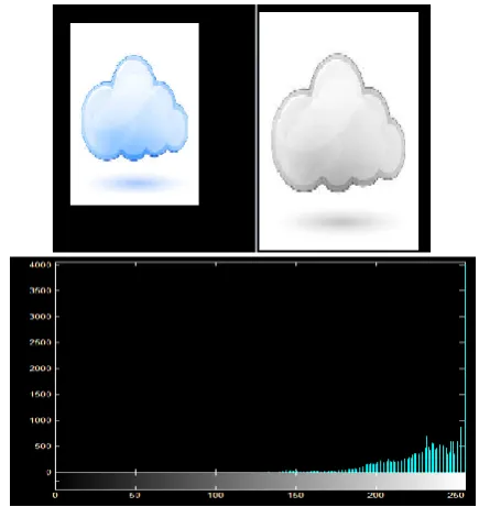
The signals which are utilized in the simulation are in the form of images. The image is encoded and then decoded using the Huffman algorithm. The algorithm will produce the result in terms of the entropy and entropy error. The result of the image is shown as

Figure 1. Showing the result of the Huffman

coding and decoding

The Huffman coding and decoding is implemented

on the other images also and desired result is

obtained. Multiple images are utilized in order to

analyze the algorithm for consistency.

Figure 2: showing the image encoding and decoding using Recursive Huffman coding

(5)

The following table shows the Iterative Huffman coding result

Entropy Entropy Error Speed Huffman Algorithm 5.067 5.789 4.567 4.892 4.557 5.087 5.769 4.527 4.110 4.235 0.566 0.899 0.987 0.456 0.787 0.564 0.829 0.787 0.356 0.487 2.223 2.122 2.234 2.123 2.222 2.987 2.673 2.323 2.099 2.876

Table 7 : Showing the Result of Recursive Huffman Coding

The proposed algorithm results are better as compared to the iterative Huffman coding.

IV. CONCLUSION

Both on real world signals and a synthetic signal the proposed Huffman coding schema does considerably better than forthright Huffman coding, and usually better than JPEG-like Huffman coding, especially at low bit rates.

V. REFERENCES

[1] Allen Gersho and Robert M. Gray. Vector

Quantization and Signal Compression. Kluwer Academic Publishers, Boston, 1992. ISBN 0-7923-9181-0

[2] Massachutilizetts Institute of Technology. The

MIT-BIH Arrhythmia Database CD-ROM, 22nd edition, 1992.

[3] Mark Nelson, Jean-Loup Gailly. The Data

Compression Book. M&T Books, New York, USA, 1996. ISBN 1-55851-434-1

[4] William B. Pennebaker, Joan L. Mitchell. JPEG:

Still Image Data Compression Standard. Van Nostrand Reinhold, New York, USA, 1992. ISBN: 0442012721

[5] Seismic Data Compression ReferenceSet.

http://www.ux.his.no/~karlsk/sdata/

[6] N. Kaur, “A Review of Image Compression Using

Pixel Correlation & Image Decomposition with,” vol. 2, no. 1, pp. 182–186, 2013.

[7] A. S. Arif, S. Mansor, R. Logeswaran, and H. A.

Karim, “Auto-shape Lossless Compression of Pharynx and Esophagus Fluoroscopic Images,” J. Med. Syst., vol. 39, no. 2, pp. 1–7, 2015.

[8] W. M. Abd-elhafiez and W. Gharibi, “Color I mage

C ompression A lgorithm B ased on the DCT B locks,” vol. 9, no. 4, pp. 323–328, 2012.

[9] R. a.M, K. W.M, E. M. a, and W. Ahmed, “Jpeg

Image Compression Using Discrete Cosine Transform - A Survey,” Int. J. Comput. Sci. Eng. Surv., vol. 5, no. 2, pp. 39–47, 2014.

[10] G. Badshah, S. Liew, J. M. Zain, S. I. Hisham, and

A. Zehra, “Importance of Watermark Lossless

Compression in Digital Medical Image

Watermarking,” vol. 4, no. 3, pp. 75–79, 2015.

[11] S. Stolevski, “Hybrid PCA Algorithm for Image

Compression,” pp. 685–688, 2010.

[12] R. C. . Gonzalez and R. E. Woods, “Digital Image

Processing,” p. 976, 2010.

[13] D. G. Sullivan and D. Ph, “Binary Trees and

Huffman Encoding Binary Search Trees Fall 2012,” 2012.

[14] T. Gebreyohannes and D. Kim, “a Daptive Noise

Reduction Scheme for Salt and Pepper.”

[15] R. H. Chan, C.-W. Ho, and M. Nikolova,

“Salt-and-Pepper noise removal by median-type noise detectors and detail-preserving regularization.,” IEEE Trans. Image Process., vol. 14, no. 10, pp. 1479–85, 2005.

[16] S. Kaisar and J. Mahmud, “Salt and Pepper Noise

Detection and removal by Tolerance based selective Arithmetic Mean Filtering Technique for image restoration,” Ijcsns, vol. 8, no. 6, pp. 271– 278, 2008.

[17] G. Nelapati, “ISSN No . 2278-3091 International

Journal of Advanced Trends in Computer Science

and Engineering Available Online at

http://warse.org/pdfs/ijatcse03132012.pdf Salt and Pepper Noise Detection and removal by Modified Decision based Unsymmetrical Trimmed Med,” vol. 1, no. 2278, pp. 93–97, 2012.

[18] A. Singh, U. Ghanekar, C. Kumar, G. Kumar, and

N. I. T. Kurukshetra, “An Efficient Morphological Salt-and-Pepper Noise Detector,” vol. 875, pp. 873–875, 2011.

[19] X. Zhang, F. Ding, Z. Tang, and C. Yu, “Salt and