Using street view imagery for 3-D survey of rock slope failures
Jérémie Voumard1, Antonio Abellán1,2, Pierrick Nicolet1,3, Ivanna Penna1,3, Marie-Aurélie Chanut4, Marc-Henri Derron1, and Michel Jaboyedoff1
1Risk analysis group, Institute of Earth Sciences, FGSE, University of Lausanne, Switzerland 2Scott Polar Research Institute, Department of Geography, University of Cambridge, UK 3Geohazard and Earth Observation team, Geological Survey of Norway (NGU), Norway 4Groupe Risque Rocheux et Mouvements de Sols (RRMS), Cerema Centre-Est, France
Correspondence to:Jérémie Voumard (jeremie.voumard@unil.ch)
Received: 31 January 2017 – Discussion started: 9 February 2017
Revised: 28 September 2017 – Accepted: 21 October 2017 – Published: 1 December 2017
Abstract. We discuss here different challenges and limi-tations of surveying rock slope failures using 3-D recon-struction from image sets acquired from street view imagery (SVI). We show how rock slope surveying can be performed using two or more image sets using online imagery with photographs from the same site but acquired at different in-stances. Three sites in the French alps were selected as pi-lot study areas: (1) a cliff beside a road where a protective wall collapsed, consisting of two image sets (60 and 50 im-ages in each set) captured within a 6-year time frame; (2) a large-scale active landslide located on a slope at 250 m from the road, using seven image sets (50 to 80 images per set) from five different time periods with three image sets for one period; (3) a cliff over a tunnel which has collapsed, using two image sets captured in a 4-year time frame. The analysis include the use of different structure from motion (SfM) pro-grams and a comparison between the extracted photogram-metric point clouds and a lidar-derived mesh that was used as a ground truth. Results show that both landslide deforma-tion and estimadeforma-tion of fallen volumes were clearly identified in the different point clouds. Results are site- and software-dependent, as a function of the image set and number of im-ages, with model accuracies ranging between 0.2 and 3.8 m in the best and worst scenario, respectively. Although some limitations derived from the generation of 3-D models from SVI were observed, this approach allowed us to obtain pre-liminary 3-D models of an area without on-field images, al-lowing extraction of the pre-failure topography that would not be available otherwise.
1 Introduction
Three-dimensional remote sensing techniques are becoming widely used for geohazard investigations due to their abil-ity to represent the geometry of natural hazards (mass move-ments, lava flows, debris flows, etc.) and its evolution over time by comparing 3-D point clouds acquired at different time steps. For example, 3-D remote sensing techniques are helping to better quantify key aspects of rock slope evolu-tion, including the accurate quantification of rockfall rates and the deformation of rock slopes before failure using both lidar (Rosser et al., 2005; Oppikofer et al., 2009; Royan et al., 2014; Kromer et al., 2015; Fey and Wichmann., 2017) and photogrammetrically derived point clouds (Walstra et al., 2007; Lucieer et al., 2013, Stumpf et al., 2015; Fernandes et al., 2016; Guerin et al., 2017; Ruggles et al., 2016).
Airborne and terrestrial laser scanners are commonly used techniques to obtain 3-D digital terrain models (Abellán et al., 2014). Despite their very high accuracy and resolution, these technologies are costly and often demanding from a lo-gistical point of view. Alternatively, structure from motion (SfM) photogrammetry combined with multi-view stereo (MVS) allows the use of end-user digital cameras to generate 3-D point clouds with a decimetre-level accuracy in a cost-effective way (Westoby et al., 2012; Carrivick et al., 2016).
which offer 360◦ panoramas from many roads, streets and other places around the world (Anguelov et al., 2013). They allow remote observation of areas without physical access to them, thus remaining cost-effective, with applications in nav-igation, tourism, building texturing, image localisation, point clouds georegistration and motion from structure from mo-tion (Zamir et al., 2010; Anguelov et al., 2010; Klingner et al., 2013; Wang et al., 2013).
The aim of the present work is to ascertain to which extent 3-D models derived from SVI can be used to detect geomor-phic changes on rock slopes.
1.1 Street view imagery
The most common SVI service is the well-known Google Street View (GSV) (Google Street View, 2017) that is avail-able from Google Maps (Google Maps, 2017) or Google Earth Pro (Google Earth Pro, 2013). We used GSV as the SVI service in this study. Alternatives include Streetside by Microsoft (Streetside, 2017) and national services like Ten-cent Maps in China (TenTen-cent Maps, 2017). SVI was first deployed in urban areas to offer a virtual navigation of the streets. More recently, non-urban zones have also been made accessible and are used for the analysis of rock slope failures in this paper.
GSV was first used in May 2007 for capturing pictures of streets of major US cities and has been deployed worldwide during the intervening years, including rural areas. GSV im-ages are collected with a panoramic camera system mounted on different types of vehicles (e.g. a car, train, bike, snowmo-bile) or carried in a backpack (Anguelov et al., 2010).
The first-generation GSV camera system was composed of eight wide-angle lenses and it is currently composed of 15 CMOS sensors of 5 Mpx each (Anguelov et al., 2010). The 15 raw images, which are not publicly available, are processed by Google to make a panorama view containing an a priori unknown image deformation (Fig. 1). A GSV panorama is normally taken at an interval of around 10 m along a linear infrastructure (road, train or path).
GSV proposes a “back-in-time” function on a certain num-ber of locations from April 2014. In addition, other histori-cal GSV images are available from 2007 for selected areas only. The number of available image sets varies greatly at dif-ferent locations: while some places have several sets, many other locations have only one image set. The back-in-time function is especially useful for natural hazards because it is possible to compare pre- and post-events images.
The GSV process can be explained in four steps (Anguelov et al., 2010; Google Street View, 2017). (1) Pictures are ac-quired in the field. (2) Images are aligned: preliminary co-ordinates are given for each picture, extracted from sen-sors on the Google car that measure GNNS coordinates, speed and azimuth of the car, helping to precisely recon-struct the vehicle path. Pictures can also be tilted and re-aligned as needed. (3) By stitching overlapping pictures,
360◦panoramas are created. Google applies a series of pro-cessing algorithms to each picture to attenuate delimitations between each picture and to obtain smooth pictures transi-tions. (4) Panoramas are draped on 3-D models to give a panorama view close to the reality; the three lidar mounted on the Google car help to build 3-D models of the scenes. Each picture of the panorama has its own internal deforma-tion, and the application of the processing chain described above causes inconstant deformation in the 360◦panorama; in addition, the end user does not have any information on or control over it.
1.2 SfM-MVS
SfM with MVS dense reconstruction is a cost-effective pho-togrammetric method to obtain a 3-D point cloud of ter-rain using a series of overlapping images (Luhmann et al., 2014). The prerequisites are that (1) the studied object is photographed from different points of view and (2) each ele-ment of the object must be captured from a minimum of two pictures, assuming that the lens deformation parameters are known in advance (Snavely, 2008; Lucieer et al., 2013). If these parameters are not known beforehand, three pictures are the minimum requirement (Westoby et al., 2012) and about six pictures are preferred. The particularity of SfM-MVS is that prior knowledge of both intrinsic camera param-eters (principal point, principal distance and lens distortion) and extrinsic camera parameters (orientation and position of the camera centre, Luhmann et al., 2014) is not needed.
The workflow of SfM-MVS normally includes the fol-lowing steps: (1) feature detection and matching (Lowe, 1999), (2) bundle adjustment (Snavely et al., 2006; Favalli et al., 2011; Turner et al., 2012; Lucieer et al., 2013), (3) dense 3-D point cloud generation (Furukawa et al., 2010; Furukawa and Ponce, 2010; James and Robson, 2012) and (4) surface reconstruction and visualisation (James and Robson, 2012).
2 Study areas and available data
We selected three study areas in France to generate point clouds from GSV images. This country was chosen be-cause GSV covers the majority of the roads and bebe-cause the timeline function works in most of the areas covered by GSV, meaning that several periods of acquisition are available. Moreover, landslide events occur regularly on French alpine roads. The aerial view of the three areas is shown in Fig. 2a and examples of corresponding GSV images are in Fig. 2b and c.
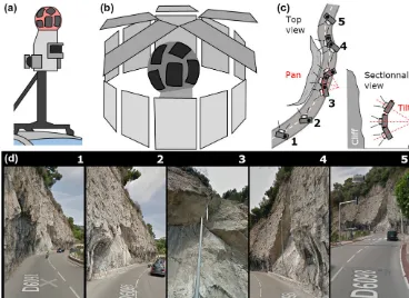
Figure 1.Google Street View (GSV) imagery functioning.(a)Schema of the GSV spherical camera system mounted on a car roof. Sen-sors in black are lidar, on to which the GSV images are draped (based on Google Street View, 2017; http://www.google.com/maps/about/ behind-the-scenes/streetview).(b)Functioning of the GSV spherical panorama built with 15 images.(c)Strategy of the GSV service for SfM-MVS photogrammetry. Numbers correspond schematically to the images in panel(d).(d)Screen captures of GSV photos from study site 1. The image numbers correspond to those in panel(c). Note the gap on the street lamp in image 3 due to the panorama construction from the GSV pictures.
with 60 GSV images taken in 2008 before the wall collapse and 50 GSV images taken in 2014 after the event.
The second case studies is the Séchilienne landslide, located 15 km southeast of Grenoble (Isère department, France). The active area threatens the departmental road RD 1091 connecting the towns of Grenoble and Briançon as well as ski resorts L’Alpe d’Huez and Les Deux Alpes to the plain. This landslide is about 800 m long by 500 m high and it has been active for more than 30 years (Le Roux et al., 2009; Durville et al., 2011; Dubois et al., 2014). The shortest dis-tance between the landslide foot and the former road is 250 m and the longest distance between the landslide head and the road is 1 km. A new road, located higher on the opposite slope, has been open since July 2016. Different SfM-MVS processes were tested, using 50–80 GSV images, at six dif-ferent times from April 2010 to June 2015.
The third case study is located in Arly gorges, between Ugine and Megève, on the path of Albertville–Chamonix-Mont-Blanc. A rockfall of about 8000 m3affected the road at the entry of a tunnel on January 2014 (France 3, 2014). Different sets of 60–110 GSV images were processed in or-der to obtain three 3-D models of the road, the tunnel entry and the cliff above the tunnel.
We used two image sets for the first study site, eight im-age sets for the second study site and four imim-age sets for the third study site, with dates ranging from May 2008 to De-cember 2016, as described in Table 1.
3 Methodology
Figure 2.The three French sites (1: Basse Corniche; 2: Séchilienne; 3: Arly gorges).(a)Google Maps aerial view of the sites (in red) with the road path (yellow) used to take the GSV images of the scenes and the view angle (blue) of the images point of view around the sites.(b)First GSV of the sites.(c)Last GSV of the sites.
To perform temporal comparisons at each site, images were taken at the different dates proposed by GSV with pre- and post-event image sets. We used the SfM-MVS pro-gram VisualSFM (Wu, 2011) for dense point cloud recon-struction for the print screen images from Google Maps and
T able 1. List of the fourteen point clouds presented in this paper . Site Figure Date Image source Image size Images Point density 1 Processing softw are Number of Comparison [pix el] number (pts m − 2) points W ith Mean SD distance 2(m) (m) Site 1 Fig. 4a May 2008 PS GSV from GM 3 1920 × 1200 60 290 V isualSFM 150 000 June 2014 7 0.2 0.7 Fig. 4b June 2014 PS GSV from GM 3 1920 × 1200 50 640 V isualSFM 182 000 May 2008 7 0.2 0.7 Site 2 Fig. 5a April 2010 PS GSV from GM 3 1920 × 1200 54 0.40 V isualSFM 18 000 Lidar 8 − 0.2 1.4 Fig. 5b March 2011 PS GSV from GM 3 1920 × 1200 52 0.25 V isualSFM 9500 Lidar 8 − 0.1 1.8 Fig. 5c May 2013 PS GSV from GM 3 1920 × 1200 45 0.37 V isualSFM 12 500 Lidar 8 − 2.1 2.7 Fig. 5d June 2014 PS GSV from GM 3 1920 × 1200 52 0.66 V isualSFM 25 000 Lidar 8 − 1.5 2.8 Fig. 5e June 2015 PS GSV from GM 3 1920 × 1200 62 0.64 V isualSFM 23 500 Lidar 8 − 0.9 3.1 Fig. 5f June 2015 GSV from GEP 4 4800 × 3500 80 0.86 V isualSFM 22 500 Lidar 8 − 1.7 3.1 Fig. 5g June 2015 GSV from GEP 3 4800 × 3500 80 1.99 Agisoft PhotoScan 236 000 Lidar 8 0.6 2.5 Fig. 5h May 2016 GoPro 5 4000 × 3000 75 0.35 Agisoft PhotoScan 46 000 Lidar 8 − 0.2 2.7 Site 3 Figs. 6a, 7a March 2010 PS GSV from GM 3 1920 × 1200 66 40 V isualSFM 35 000 Lidar 9 0.0 0.5 Figs. 6b, 7b July 2014 PS GSV from GM 3 1920 × 1200 111 50 V isualSFM 53 000 Lidar 9 0.1 0.7 Figs. 6c, 7c August 2016 GSV from GEP 2 4800 × 3107 64 2200 Agisoft PhotoScan 3 185 000 Lidar 9 − 0.1 0.7 Fig. 6d December 2016 GoPro 6 4000 × 3000 50 650 Agisoft PhotoScan 2 217 000 Lidar 9 0.0 0.4 1Point density around a search radius of 2 m. 2A v erage distance between the mesh of the reference point cloud and the compared point cloud using the point-to-mesh strate gy . 3Print screens (PS) of Google Street V ie w (GSV) from Google Maps (GM). 4GSV images sa v ed in Google Earth Pro (GEP). 5GoPro Hero4 + . 6GoPro Hero5 Black with GNSS chip inte grated. 7Comparison between the entire point clouds of May 2008 and June 2014 (Fig. 4d). 8Comparison with the 50 cm airborne lidar digital ele v ation model (DEM) from 2010. 9Comparison with the December 2016 lidar DEM (6 930 000 points) without v egetation from an assembly of six Optech terrestrial lidar clouds.
Figure 3.Flowchart of the SfM-MVS processing with GSV im-ages on an area with the back-in-time function available. Pre-event images are displayed using the back-in-time function in GSV. Post-event images arise either from print screens of GSV in Google Maps using or not the back-in-time function or from GSV images saved in Google Earth Pro. In this last case, the last available proposed GSV images have a greater resolution as the print screens and can be pro-cessed in the Agisoft PhotoScan.
lidar scans for sites 2 and 3) and then the other point cloud was compared to this reference mesh. The computed short-est distance, a signed value, between the mesh and the point cloud is the length of the 3-D vector from the mesh triangle to the 3-D point. Thus, average distances and standard devi-ations for each comparison of point clouds were computed. Point density of point clouds was obtained using the “point density” function in CloudCompare with the “surface den-sity” option.
Beside the images taken from print screens as described above, we also obtained GSV images (4800×3500 pixels, 16.8 Mpx) from Google Earth Pro on sites 2 and 3 with the “save image” function. This second way to get GSV allows us to get images with a higher resolution than print screen images. Unfortunately, there is no timeline (or back-in-time) function in Google Earth Pro; it is only possible to save im-ages from the last picture acquisition, i.e. generally post-event images. GSV images from Google Earth Pro were pro-cessed with the Agisoft PhotoScan software (Agisoft, 2015) for dense point cloud reconstruction, which provides much better results than VisualSFM. GSV images from Google Map were processed with VisualSFM because Agisoft was not able to process those print screens. The flowchart of Fig. 3 shows the processing applied to both types of images (print screens and saved images).
extracted from Google Maps or from the French geoportal (Géoportail, 2016) and without ground control points.
It is important to mention here that a series of issues is expected when attempting to use SVI for 3-D model recon-struction with SfM-MVS. GSV images are constructed as 360◦panoramas from a series of pictures, so the internal de-formation of the original image is not fully retained on the panoramas. In other words, the deformation of a cropped sec-tion of the panorama will be a main funcsec-tion not only of the internal deformation of the camera and lens but also of the panorama reconstruction process; this circumstance will sig-nificantly influence the bundle adjustment process and thus the 3-D reconstruction.
In addition, GoPro Hero4+images from a moving vehicle on the road were taken by the authors at site 2, as well a se-ries of images captured using a GoPro Hero5 Black camera standing on site 3 (image resolution of 4000×3000 pixels, 12 Mpx). Six lidar scans were also taken at site 3. This infor-mation was used for quality assessment purposes.
4 Results and discussion
Different results are obtained depending on the software used for SfM-MVS processing. For all case studies, Visu-alSFM gave results with print screens from GSV in Google Maps while Agisoft PhotoScan could not align those print screens despite adding a series of control points measured with Google Earth Pro. Resolution of print screen images seem to be insufficient for processing with Agisoft Photo-Scan. However, with higher point density and empty areas, Agisoft PhotoScan provided better results with images from Google Earth Pro than VisualSFM.
4.1 Site 1 – Basse Corniche site
It was possible at the Basse Corniche site to estimate the fallen volume by scaling and comparing the 2008 (Fig. 4a) and 2010 (Fig. 4b) point clouds. The 2008 point cloud is composed of 150 000 points with an average density of 290 points m2, and the 2014 point cloud is composed of 182 000 points with an average density of 640 points m2 (Ta-ble 1). VisualSFM could align the images and make 3-D models before and after the wall collapse. It was possible to roughly scale and georeference the scene with the road width and a few point coordinates measured on Google Earth Pro or on the French geoportal. After aligning the two 3-D point clouds, meshes were built to compute the collapsed volume. The point-to-mesh alignment in CloudCompare of both point clouds was done on a small, stable part of the cliff (Fig. 4c) with a standard deviation of the point-to-mesh distance of about 10 cm (Fig. 9 and Table 2) and on the entire cliff be-side the vegetation with a standard deviation of about 25 cm (Fig. 4e). In the collapsed area, the maximal horizontal dis-tance between the two datasets is about 3.9 m (indicated in
red in Fig. 4d). The collapsed volume (including a possible empty space between the cliff and the wall before the event) was estimated to be about 225 m3using the point cloud com-parison. Based on Google Street images, we manually es-timated the dimensions of this volume (15 m long×10 m high×1.5 m deep), getting a similar value.
The obtained point clouds at site 1 allow us to detect ob-jects of a few decimetres. This accuracy was adequate to es-timate the collapsed volume with an accuracy similar to the estimation made by hand based on the GSV photos and dis-tances measured on Google Earth Pro and the French geo-portal. This relatively high accuracy is due to the following factors: good image quality, reduced distance between the cliff and camera locations, good lighting conditions, absence of obstacles between the camera location and the area under investigation, no vegetation and efficient repartition of point of view around the cliff (Fig. 2a).
4.2 Site 2 – Séchilienne landslide
Eight point clouds, of which seven were derived through the SfM-MVS process with GSV images, were generated for the Séchilienne landslide at six different time steps (from April 2010 to June 2015). Three different image sources were used: GSV print screens from Google Maps, GSV im-ages saved from Google Earth Pro and imim-ages from a Go-Pro HERO4+ camera from a moving vehicle (Fig. 5 and Table 1). Two different programs (VisualSFM and Agisoft PhotoScan) were used for image treatment depending on the image sources (Fig. 3 and Table 1). The number of 3-D points on the landslide area varies from 9500 to 22 500 points for a processing with VisualSFM with an average density of 0.25 to 0.85 points m2, while 236 000 3-D points were generated when using Agisoft PhotoScan with an average density of 2 points m2(Table 1). In comparison, 1 500 000 points were obtained on the same area using terrestrial photogrammetry with a 24 Mpx reflex camera.
Results were aligned on a 50 cm resolution airborne lidar scan of the landslide acquired in 2010. Then, the street view SfM-MVS point clouds were aligned and compared with a mesh from the lidar scan using the point-to-mesh strategy. The alignment between the lidar point cloud and SfM-MVS point clouds derived from SVI is a key factor to define the quality of the cloud comparison. This alignment on stable areas (manually selected) was not easy to perform because of the low density of points on the SfM-MVS clouds derived from SVI. We noted a huge difference in the number of points between the different SfM-MVS clouds derived from SVI. This difference in the number of points shows the impact of the image quality. Images with a good quality (resolution, exposition, sharpness) will give point clouds with a higher number of points as point clouds from low-quality images.
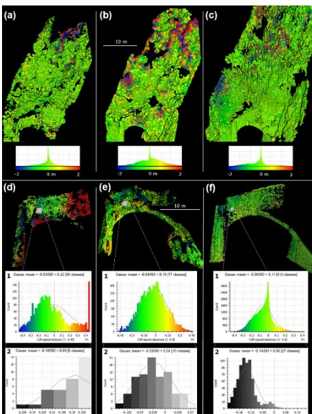
Figure 4. Results at site 1, Basse Corniche. (a) Three-dimensional model produced with GSV images taken before the event in 2008. (b)Three-dimensional model produced with GSV images taken after the event in 2014.(c)Statistics on a small part of the wall (red polygon in paneld) of 7510 points between the two point clouds with the point-to-mesh strategy in the CloudCompare.(d)Comparison of the two point clouds of 2008 and 2014 on the entire surface of the 3-D point clouds. The maximal horizontal depth of the cliff is about 3.9 m.(e)Comparison of the two point clouds of 2008 and 2014 on the entire stable parts of the cliff (i.e. without vegetation) by not taking into account the collapsed wall (black triangle in the centre of the point clouds). The information on the picture source, date, point density and program used is given in Tables 1 and 2.
and Table 1). The 2010 point cloud (Fig. 5a2) compared with the 2010 lidar scan does not show any significant changes. Small orange and red dots are spread out on the entire land-slide surface suggesting artefacts and not a real slope change. The 2010–2011 point cloud comparison (Fig. 5b2) shows lit-tle red (material accumulation) in the deposition and in the failure areas. The 2016 point cloud (Fig. 5c2) highlights ma-terial deposition in red, in the left part. This is confirmed by a comparison of a 2013 terrestrial lidar. The blue pattern indicates a loss of material in the failure and the toe areas. The 2014 point cloud (Fig. 5d2) shows similar results to the 2013 point cloud but with a light increase of material in the deposition area and rock loss in the failure area. The 2010 to 2014 point clouds (Fig. 5a–d) were processed with Visu-alSFM with GSV print screens in Google Maps (Table 1).
T able 2. List of the eight partial point cloud comparisons. Site Figure Date Image source Image size Processing Comparison (pix el) softw are Comparati v e area W ith Mean distance 1(cm) Site 1 Fig. 4c May 2008 PS GSV from GM 2 1920 × 1200 V isualSFM Small clif f part June 2014 0 Fig. 4e May 2008 PS GSV from GM 2 1920 × 1200 V isualSFM Entire clif f without w all and v egetation June 2014 22 Site 3 Fig. 7d1 March 2010 PS GSV from GM 2 1920 × 1200 V isualSFM T unnel entr y Lidar 4 − 3 Fig. 7d2 March 2010 PS GSV from GM 2 1920 × 1200 V isualSFM Small part of tunnel entry Lidar 4 − 18 Fig. 7e1 July 2014 PS GSV from GM 2 1920 × 1200 V isualSFM T unnel entry Lidar 4 − 4 Fig. 7e2 July 2014 PS GSV from GM 2 1920 × 1200 V isualSFM Small part of tunnel entry Lidar 4 − 3 Fig. 7f1 August 2016 GSV from GEP 3 4800 × 3107 Agisoft PhotoScan T unnel entry Lidar 4 − 6 Fig. 7f2 August 2016 GSV from GEP 3 4800 × 3107 Agisoft PhotoScan Small part of tunnel entry Lidar 4 − 14 1A v erage distance between the mesh of the reference point cloud and the compared point cloud using the point-to-mesh strate gy . 2Print screens (PS) of Google Street V ie w (GSV) from Google Maps (GM). 3GSV images Google Earth Pro (GEP). 4Comparison with the December 2016 lidar digital ele v ation model (6 930 000 points) without v egetation from an assembly of six Optech terrestrial lidar clouds.
point cloud is very similar to the 2016 GoPro point cloud (Fig. 5h2), which confirms the results of SfM-MVS process-ing with GSV images.
Results of site 2 show that images with low resolution and with low lighting generated a lower number of points compared to the models generated with the last generation of GSV cameras, having higher resolution, more advanced sensors and pictures taken with favourable lighting condi-tions. The large distance between the road and the landslide considerably limits the final accuracy due to low image reso-lution, as discussed in Eltner et al. (2016); the closest dis-tance between the road and the centre of the landslide is 500 m and the largest distance between the upper part of the landslide and the point of view is about 1400 m. Furthermore, the vegetation on the landslide foot and along the road as well as a power line partially obstruct the visibility of the study area. In addition, clouds are present on several images on the top of the scarp, degrading the upper part of the 3-D point cloud.
4.3 Site 3 – Arly gorges
Four point clouds, of which three were derived from the SfM-MVS process using GSV images, were generated at the Arly gorges site at four different times (from March 2010 to December 2016). Three different image sources (GSV print screens from Google Maps, GSV images exported from Google Earth Pro and our own images acquired from a GoPro HERO5 Black) were used (Fig. 6 and Table 1). Two different programs (VisualSFM and Agisoft PhotoScan) were tested. In addition, a lidar point cloud resulting from an assembly of six Optech ILRIS scans has been used as ground truth (Fig. 6e). The number of points varies from 35 000 points to 3.2 million points with an average density of 40 to 2 200 points m2(Table 1).
Figure 6.Results at site 3, the Arly gorges. Five point clouds from four different image sets sources and processed with two different softwares and one lidar scan.(a)March 2010 point cloud.(b)July 2014 point cloud.(c)August 2016 point cloud.(d)December 2016 point cloud taken on foot with a GoPro camera.(e)December 2016 lidar cloud from an assembly of six Optech terrestrial lidar scans. The grey elements in the cliff are the protective nets.
not the case on the 2010 point cloud. The point cloud pro-cessed in Agisoft PhotoScan derived from 2016 GSV images saved from Google Earth Pro displays much better quality than the previous (Figs. 6c and 7c): we now see the protec-tive nets in the slope as well as the blue road sign announcing the tunnel. The vegetation is also observable and the tunnel entry is similarly modelled as the 2016 GoPro point cloud (Fig. 6d).
The SfM-MVS point cloud derived from GoPro images gives a significantly better representation of the whole scene, especially on the top of the model. Slope structures and pro-tective nets are well modelled, but the small vegetation is not. The comparison between the 2016 lidar scan (Fig. 6e) and the three SfM-MVS with GSV images point clouds does not al-low us to identify terrain deformation on the cliff. Moreover, the source area of the rockfall is not observable from the GSV images because it is located higher in the slope, outside of the images.
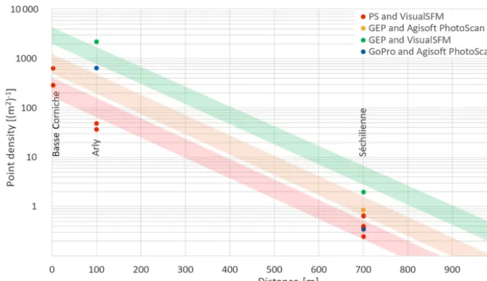
Figure 8.Correlation between the distance from the camera to the case studies and the expected density of points from the three case studies. The red dots are results of the three case studies point clouds obtained from Google Street View (GSV) print screens (PS) in Google Maps (GM) processed with VisualSFM. The red strip represents the corresponding trend based on a negative exponential function. The orange dot is the result of the Séchilienne point cloud obtained from GSV images saved in Google Earth Pro (GEP) processed with VisualSFM. The orange strip represents the corresponding trend based on a negative exponential function. The green dots are the results of the Séchilienne and Arly point clouds obtained from GSV images saved in GEP, processed with Agisoft PhotoScan. The green strip represents the corresponding trend based on a negative exponential function. To compare, the blue dots represent the result of the Séchilienne and Arly point clouds obtained with GoPro action camera images taken on the field and processed with Agisoft PhotoScan.
prove the processing. Information on the picture source, date, point density and program used is given in Table 1.
A strong limiting factor at this site is the non-optimal cam-era locations. Indeed, the location of the cliff above a tun-nel portal does not allow for a lateral movement between the camera positions with regard to the cliff. The maximal view-ing angle (in blue in Fig. 2a) is about 35◦compared to 170◦ for site 1 and 115◦for site 2, i.e. 3 to 5 times smaller than for the other studied sites.
4.4 Discussion
With the experience acquired during the research, we can highlight the following recommendations to improve results of SfM-MVS with SVI images. (a) Firstly, the distance be-tween the image point of view and the subject as well as the size of the subject are important because they influence the pixel size of the subject. In case study 1, the location of the cliff next to the road (< 1 m) allows us to get images with a good resolution for the studied object. In case study 2, the area under investigation is too far from the road (500– 1400 m) and small structures cannot be seen in the landslide. (b) Secondly, the ability to look at the scene from different angles (Fig. 2a) is a determining factor to obtain good results. The greater this viewing angle is, the better the results will be. Case study 1 with a view angle of almost 180◦is optimal because the object is observable from half a circle. The view angle of case study 2 (115◦) is enough to get many different
views of the subject from different angles. The view angle is too narrow to have enough different points of view of the cliff in case study 3 (35◦). (c) Thirdly, results are influenced by the image quality and especially by their exposition, con-trast and type of sensor, which have been progressively im-proved during the last few years. Image quality varies consid-erably for different image sets. Case study 1 is again the best study case in term of image quality. Both image sets have optimal solar exposition and shadows are not strong. Case study 2 has sets with very different images quality. Some sets are well exposed, while others are not. Clouds are present on few image sets. For case study 3, we have a lot of over- and underexposed images due to the location of the site (incised valley with a southwest-oriented slope with a lot of light or shadow). The problem of image quality must concern Google too since the company removed very underexposed GSV im-ages taken in August 2014 at site 3 from Google Maps at the end of 2016.
ar-Figure 9.Correlation between the distance from the camera to the case studies and the expected standard deviation from the three case studies. The dots are results of point cloud comparisons on the en-tire point cloud areas (Table 1). The triangles are the results of point cloud comparisons on partial point cloud area (Table 2). The red dots and triangles are the results of the three case studies’ point clouds obtained from Google Street View (GSV) print screens (PS) in Google Maps (GM), processed with VisualSFM compared on the entire area. The orange dot is the result of the Séchilienne point cloud obtained from GSV images saved in Google Earth Pro (GEP) processed with VisualSFM. The green dots and triangles are the re-sults of the Séchilienne and Arly point clouds obtained from GSV images saved in GEP, processed with Agisoft PhotoScan. To com-pare, the blue dots represent the result of the Séchilienne and Arly point clouds obtained with GoPro action camera images taken on the field and processed with Agisoft PhotoScan.
eas show interesting results when the point cloud alignment is well done. Thus, we observed standard deviations of a few decimetres in stable areas at site 1 (Fig. 3d), between 0.5 and 1.1 m at site 2 and between 11 and 22 m at the tunnel entry on site 3. Standard deviations increase at site 2 when point clouds are compared to their entire surface (Fig. 5a2–h2, Ta-ble 1). This is attributaTa-ble to the occurrence of slope move-ments generating material increase or decrease and thereby increasing standard deviations of the distance between the two compared point clouds. It can also be due to a bad 3-D point cloud alignment. Indeed, cloud alignment is not al-ways easy on some point clouds because of low point density, voids in the point clouds (like in the landslide toe in Fig. 5f2) and the roughness of the terrain. In such difficult alignment cases, we tried to align the point clouds on stable parts where point density was high.
Our study highlighted important differences in 3-D model reconstruction using different software, comparing with
pre-ages from Google Earth Pro (Fig. 5f–g) and pictures acquired from a GoPro Hero camera (Fig. 5h). Nevertheless, Visu-alSFM performed better than Agisoft PhotoScan on print screen captures from SVI. The only difference between these sources of information is the resolution: 2.3 Mpx for print screens from Google Maps, 16.8 Mpx for images saved from Google Earth Pro and 12 Mpx for GoPro camera, stressing the importance of picture resolution to the quality of the 3-D model.
The point density was evaluated according to the distance between the image point of view and the subject and the im-age types and processing software. The obtained results and the derived trends indicate that the use of GSV images from Google Earth Pro with VisualSFM increases the point den-sity by a factor of 2 compared to the processing of GSV print screens with VisualSFM. The processing of GSV images from Google Earth Pro with Agisoft PhotoScan increases the point density by a factor of 10 compared to the process-ing of GSV print screens with VisualSFM (trend strips in Fig. 8). The expected point density of the 3-D point clouds from GSV print screens processed in VisualSFM of a subject located a few metres from the camera (Basse Corniche dots in Fig. 8) is about 300 points m−2, about 50 points m−2for an area located at about 100 m (Arly dots in Fig. 8) and about 0.5 point m−2for an area located at about 700 m (Séchilienne dots in Fig. 8).
A simple development to improve our proposed approach would be for Google to add the back-in-time function to Google Earth Pro. In this case, it would be possible to save GSV images from any proposed time period and to process those images with Agisoft PhotoScan (Fig. 5g) and thus obtain better results than using VisualSFM (Fig. 5f). Since Google services and functionalities of Google Maps and Google Earth evolve over time, it is possible that SfM-MVS with GSV images will be more efficient and easier in the near future.
5 Conclusions
In this study it was possible to detect and characterise small landslides and rockfalls (< 0.5 m3)for study areas relatively close to the road (from 0 to 10 m); complementarily, it was possible to detect large-scale landslides or rock collapses (> 1000 m3)over areas located far away from the road (100 m or more). This information is of great interest when no other data of the studied area have been obtained.
The proposed methodology provides interesting but chal-lenging results due to some constraints linked to the quality of the input imagery. The inconsistent image deformations and the impossibility of extracting the original images from a street view provider are the most important limitations for 3-D model reconstruction derived from SVI. The following constraints strongly limit the proposed approach: large dis-tances between the camera position and the subject of in-vestigation, presence of obstacles between the studied area and the road, image quality, poor meteorological conditions, non-optimal images repartition, reduced number of images, and the existence of shadows and/or highlighted areas. The quality of the final product was observed to be mainly de-pendent on the image quality and the distance between the studied area and image perspectives.
Despite the abovementioned limitations, SfM-MVS with SVI can be a useful tool in geosciences to detect and quantify slope movements and displacements at an early stage of the research by comparing datasets taken at different time series. The main interest of the proposed approach is the possibility to use archival imagery and deriving 3-D point clouds of an area that has not been captured before the occurrence of a given event. This will allow expanding the database on rock slope failures, especially for slope changes along roads with conditions that are favourable for the proposed approach.
Data availability. Point cloud data presented used in this paper are
available on demand.
Competing interests. The authors declare that they have no conflict
of interest.
Acknowledgements. The second author was funded by the H2020
Program of the European Commission through Marie Skłodowska-Curie Individual Fellowships (MSCA-IF-2015-705215).
Edited by: Thomas Glade
Reviewed by: Olga Mavrouli and Matt Lato
References
Abellán, A., Oppikofer, T., Jaboyedoff, M., Rosser, N. J., Lim, M., and Lato, M. J.: Terrestrial laser scanning of rock slope instabil-ities, Earth Surf. Proc. Land., 39, 80–97, 2014.
Agisoft, L. L. C.: Agisoft PhotoScan user manual, Professional edi-tion, version 1.2.6, 2015.
Anguelov, D., Dulong, C., Filip, D., Frueh, C., Lafon, S., Lyon, R., Ogale, A., Vincent, L., and Weaver, J.: Google Street View: Cap-turing the world at street level, Computer, 43, 32–38, 2010. Carrivick, J. L., Smith, M. W., and Quincey, D. J.: Structure from
Motion in the Geosciences, John Wiley & Sons, Pondicherry, In-dia, 2016.
Dubois, L., Chanut, M.-A., and Duranthon, J.-P.: Amélioration con-tinue des dispositifs d’auscultation et de surveillance intégrés dans le suivi du versant instable des Ruines de Séchilienne, Géo-logues, 182, 50–55, 2014.
Durville, J.-L., Bonnard, C., and Potherat, P.: The Séchilienne (France) landslide: a non-typical progressive failure implying major risks, J. Mt. Sci., 8, 117–123, 2011.
Eltner, A., Kaiser, A., Castillo, C., Rock, G., Neugirg, F., and Abel-lán, A.: Image-based surface reconstruction in geomorphometry – merits, limits and developments, Earth Surf. Dynam., 4, 359– 389, https://doi.org/10.5194/esurf-4-359-2016, 2016.
Favalli, M., Fornaciai, A., Isola, I., Tarquini, S., and Nannipieri, L.: Multiview 3D reconstruction in geosciences, Computers & Sci-ences, 44, 168–176, 2011.
Fey, C. and Wichmann, V.: Long-range terrestrial laser scan-ning for geomorphological change detection in alpine terrain – handling uncertainties, Earth Surf. Proc. Land., 42, 789–802, https://doi.org/10.1002/esp.4022, 2017.
Fernández, T., Pérez, J. L., Cardenal, J., Gómez, J. M., Colomo, C., and Delgado, J.: Analysis of Landslide Evolution Affecting Olive Groves Using UAV and Photogrammetric Techniques, Remote Sens., 8, 837, https://doi.org/10.3390/rs8100837, 2016. Furukawa, Y. and Ponce, J.: Accurate, dense, and robust multiview
stereopsis, IEEE T. Pattern Anal., 32, 1362–1376, 2010. Furukawa, Y., Curless, B., Seitz, S. M., and Szeliski, R.: Towards
internet-scale multi-view stereo, Computer Vision and Pattern Recognition (CVPR), 2010 IEEE Conference, 1434–1441, IEEE, 2010.
France 3 : Important éboulement dans les gorges de l’Arly en Savoie, available at : http://france3-regions.francetvinfo.fr (last access: 25 January 2017), 2014.
Géoportail: IGN (2016), available at: http://www.geoportail.gouv.fr (last access: 25 January 2017), 2016.
Girardeau-Montaut, D.: CloudCompare (version 2.9), GPL soft-ware, available at: http://www.cloudcompare.org (last access: 28 November 2017), 2011.
Google Street View: Understand Street View, 2017, available at: https://www.google.com/maps/streetview/understand, last ac-cess: 25 January 2017.
Google Maps: Google Inc. (2017), available at: https://maps.google. com, last access: 25 January 2017.
Google Earth Pro: version 7.1.2.241, Google Inc. (2013), avail-able at: https://www.google.com/earth (last access: 28 November 2017), 2013.
Guerin, A., Abellán, A., Matasci, B., Jaboyedoff, M., Derron, M.-H., and Ravanel, L.: Brief communication: 3-D reconstruction of a collapsed rock pillar from Web-retrieved images and ter-restrial lidar data – the 2005 event of the west face of the Drus (Mont Blanc massif), Nat. Hazards Earth Syst. Sci., 17, 1207– 1220, https://doi.org/10.5194/nhess-17-1207-2017, 2017. James, M. R. and Robson, S.: Straightforward reconstruction
of 3D surfaces and topography with a camera, Accuracy and geosciences application, J. Geophys. Res., 117, F03017, https://doi.org/10.1029/2011JF002289, 2012.
Klingner, B., Martin, D., and Roseborough, J.: Street View Motion-from-Structure-from-Motion, Proceedings of the International Conference on Computer Vision, IEEE, 2013.
Kromer, R., Abellán, A., Hutchinson, J., Lato, M., Edwards, T., and Jaboyedoff, M.: A 4D Filtering and Calibration Tech-nique for Small-Scale Point Cloud Change Detection with a Terrestrial Laser Scanner, Remote Sens., 7, 13029–13052, https://doi.org/10.3390/rs71013029, 2015.
Le Roux, O., Schwartz, S., Gamond, J. F., Jongmans, D., Bourles, D., Braucher, R., Mahaney, W., Carcaillet, J., and Leanni, L.: CRE dating on the head scarp of a major landslide (Séchilienne, French Alps), age constraints on Holocene kinematics, Earth Planet. Sc. Lett., 280, 236–245, 2009.
Lowe, D.: Object recognition from local scale-invariant features, International Conference of Computer Vision, Corfu Greece, 1150–1157, 1999.
Lucieer, A., de Jong, S., and Turner, D.: Mapping landslide dis-placements using Structure from Motion (SfM) and image cor-relation of multi-temporal UAV photography, Prog. Phys. Geog., 38, 97–116, 2013.
Luhmann, T., Robson, S., Kyle, S., and Boehm, J.: Close-range pho-togrammetry and 3D imaging, Walter De Gruyter, Berlin/Boston, 2014.
Micheletti, N., Chandler, J. H., and Lane, S. N.: Investigating the geomorphological potential of freely available and accessi-ble Structure-from-Motion photogrammetry using a smartphone, Earth Surf. Proc. Land., 40, 473–486, 2015.
Nice-Matin : La basse corniche coupée en direc-tion de Monaco après un éboulement, available at : http://www.nicematin.com/menton/ (last access: 15 Octo-ber 2015), 2014.
Niederheiser, R., Mokroš, M., Lange, J., Petschko, H., Prasicek, G., and Elberink, S. O.: Deriving 3d Point Clouds from Terrestrial Photographs-Comparison of Different Sensors and Software. In-ternational Archives of the Photogrammetry, Remote Sensing and Spatial Information Sciences-ISPRS Archives, 41, 685–692, 2016.
Rosser, N. J., Petley, D. N., Lim, M., Dunning, S. A., and Allison, R. J.: Terrestrial laser scanning for monitoring the process of hard rock coastal cliff erosion, Q. J. Eng. Geol. Hydroge., 38, 363– 375, 2005.
Royán, M. J., Abellán, A., Jaboyedoff, M., Vilaplana, J. M., and Calvet, J.: Spatio-temporal analysis of rockfall pre-failure defor-mation using Terrestrial LiDAR, Landslides, 4, 697–709, 2014. Ruggles, S., Clark, J., Franke, K. W., Wolfe, D., Reimschiissel,
B., Martin, R. A., Okeson, T. J., and Hedengren, J. D.: Com-parison of SfM computer vision point clouds of a landslide de-rived from multiple small UAV platforms and sensors to a TLS-based model, Journal of Unmanned Vehicle Systems, 4, 246– 265, 2016.
Snavely, N.: Scene reconstruction and visualization from Internet photo collections, unpublished PhD thesis, University of Wash-ington, USA, 2008.
Snavely, N., Seitz, S. M., and Szeliski, R.: Photo Tourism: Explor-ing Photo Collection in 3D, SIGGRAPH, 6, 835–846, 2006. Snavely, N., Seitz, S., and Szeliski, R.: Modeling the World from
In-ternet Photo Collections Int. J. Comput Vision, Springer Nether-lands, 80, 189–210, 2008.
Streetside: Microsoft Inc. (2017), available at: https://www. microsoft.com/maps/streetside.aspx, last access: 25 January 2017.
Stumpf, A.: Ground-based multi-view photogrammetry for the monitoring of landslide deformation and erosion, Geomorphol-ogy, 231, 130–145, 2015.
Tencent Maps: Tencent Inc. (2017), available at: http://map.qq.com, last access: 25 January 2017.
Turner, D., Lucieer, A., and Watson, C.: An Automated Technique for Generating Georectified Mosaics, from Ultra-High Resolu-tion Unmanned Aerial Vehicle (UAV), Conference on 3D Imag-ing, ModelImag-ing, ProcessImag-ing, Visualization & Transmission Im-agery, Based on Structure from Motion (SfM) Point Clouds, Re-mote Sensing, 4, 1392–1410, 479–486, 2012.
Walstra, J., Chandler, J. H., Dixon, N., and Dijkstra, T. A.: Aerial photography and digital photogrammetry for landslide monitor-ing, Geological Society, London, Special Publications, 283, 53– 63, 2007.
Wang, C.-P., Wilson, K., and Snavely, N.: Accurate Georegistration of Point Clouds Using Geographic Data, 3D Vision – 3DV, IEEE, 33–40, 2013.
Westoby, M. J., Brassington, J., Glasser, N. F., Hambrey, M. J., and Reynolds, J. M.: “Structure-from-Motion” photogrammetry: A low-cost, effective tool for geoscience applications, Geomor-phology, 179, 300–314, 2012.
Wu, C.: VisualSFM: A visual structure from motion system, avail-able at: http://ccwu.me/vsfm (last access: ä 25 January 2017), 2011.