The application of 3D image registration techniques in diagnosis and therapy

(1)

The application of 3D image registration

techniques in diagnosis and therapy

Jin g Yi W ang

A rep o rt su b m itte d to the U n iv e rsity C o lleg e L ondon

fo r the aw ard o f the q u lifie d to the M phil degree

2001

D ep artm en t o f M ed ical P h y sics and B io e n g in e erin g

U n iv e rsity C o llege

(2)

INFORMATION TO ALL U SE R S

The quality of this reproduction is d ep en d en t upon the quality of the copy subm itted.

In the unlikely even t that the author did not sen d a com plete manuscript

and there are m issing p a g e s, th e se will be noted. Also, if material had to be rem oved, a note will indicate the deletion.

uest.

ProQ uest U 644156

Published by ProQ uest LLC(2016). Copyright of the Dissertation is held by the Author.

This work is protected against unauthorized copying under Title 17, United S ta tes C ode. Microform Edition © ProQ uest LLC.

ProQ uest LLC

789 East E isenhow er Parkway P.O. Box 1346

(3)

A bstract

In recent years, rapid developments in medical 3D scanner technology have led to a major

increase in the amount of information available to the physician. Image data are acquired

ushg techniques like CT, MR, SPECT and PET. In this thesis, I will give a general review of

the base technique of registration and its clinical applications; report on using an image fusion

technique to integrate these 3D multimodality images to develop a clinical therapy planning

tod.

The first aim of my project was to investigate the use of different kinds of registration

methods on a group of children. Different kinds of registration methods are reviewed. The

clinical on applications are discussed and some of our new work is reported.

The second aim of our project was to produce registered and subtracted ictal and interictal

SPECT images obtained from the children. In order to highlight the lesions, the transformed,

noimalised interictal images were subtracted from the normalised ictal image to create an

image where the value for each pixel represents the intensity difference between the two data

sets. The standard deviation (SD) of the distribution of the subtraction pixel intensities was

calculated, and the subtraction image thresholded to display only pixels with values greater

than 2 SDs above zero. Ictal SPECT provides unique information on the dynamic changes in

regional cerebral blood flow (rCBF) that occur during seizure and, thus, could be useful in

clarifying the poorly understood interplay of the interictal states in human focal epilepsy. The

results were compared with the visual diagnosis and surgical outcome and enhanced the

ability to localize the seizure foci.

The future work will be based on improving the accuracy of the method of normalisation.

The threshold range selection will be further investigated for different injection times. The

size of the subtraction image highlights which correspond to the lesions will need further

(4)

I would like to thank my principal supervisor Dr. A.D.Linney for his great support and

encouragement throughout the duration of this thesis. I am also grateful my second supervisor

Dr. Cliff Ruff for his helpful suggestions. There are many friends and colleagues who

provided invaluable encouragement both on a practical and emotional level. In particular, I

would like to thank Dr. Jing Deng for his friendship when I first arrived at the Medical

Graphics and Imaging Group and for patiently teaching me the basic knowledge of how to use the computer and software. I am also grateful to the people in the Medical Graphics and

Imaging Group for their support. I would also like to thank Dr. Isky Gordon for providing me

with the SPECT data and related clinical information.

Finally but not at least I would like to thank my husband lie Sun for his financial support

(5)

List of Figures

F ig 2 .1 ...17

F ig 2.2 ... 19

F ig 2 .3 ... 20

F ig 2 .4 ...24

F ig 2 .5 ...29

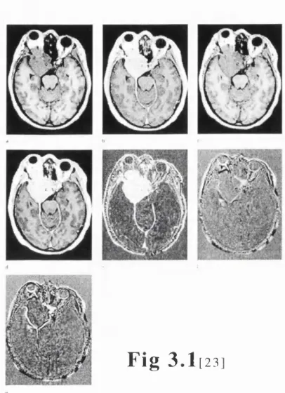
F ig 3.1 ... 39

Fig 3.2 ... 40

Fig 3.3 ... 42

Fig 3.4 ... 46

F ig 3.5 ... 47

F ig 4 .1 ...54

Fig 4 .2 ... 54

Fig 4.3 ... 59

Fig 4 .4 ...60

Fig 4.5 ... 66

Fig 4 .6 ...67

Fig 5 .1 ...75

Fig 5 .2 ...76

Fig 5 .3 ...77

(10)

Vm T he set o f p o in ts m aking up th e volum e of m a teria l im aged by

m o d a lity M

m (x),n(x) The u n d e rly in g v alu e e x h ib ite d by a m ateria l at lo c a tio n x

m (x ),n (x ) T he m e asu red v alu e of a p h y sica l p ro p e rty at lo c a tio n x

R The set o f reg io n s of m a te ria l m aking up a scene bein g im aged

k,K A set o f p o in ts m aking up a reg io n in the im age all e x h ib itin g the

sam e v alu e o f a p ro p erty

M ,N S ets o f v alu es o f p ro p e rtie s e x h ib ite d m a te ria ls in a scene

p(m ) P ro b a b ility of a value m o cc u rrin g w ith in an im aged scene

M ,N S ets o f m easu rem en t values

p(m ) P ro b a b ility o f a m easu rem en t v alu e m o ccu rrin g w ith in an im age

T A tra n sfo rm a tio n m apping b etw een tw o 3D im ages o f a scene

5 ‘ n(m j N o rm a lise d sta n d a rd d e v ia tio n of c o rre sp o n d in g im age

v alu es N w ith re sp e c t to the im age valu es M

H(M ) E n tro p y o f a set o f sym bols m e M

H (M ,N ) J o in t en tro p y b etw een sets of m easu red valu es M and N

I(M ,N ) M u tu al in fo rm a tio n b etw een sets o f m easu red values M and N

Y(M,N) N o rm a lise d M utual in fo rm a tio n b etw een sets o f m easu red v alu es M

(11)

List of Abbreviations

3D T h ree D im en sio n a l

2D Two D im e n sio n a l

C B F C e re b ra l B lo o d Flow

CT (X -ray ) C o m p u ter T om ography

EEG E le c tro e n c e p h a lo g ra p h y

EDO F lu o ro d e o x y g lu c o se R a d io p h a rm ac e u tic a l used in PET im ag in g

ERE F id u c ia l R e g istra tio n E rro r

FW HM F ull W id th at H a lf M axim um

HM PA O H e x a m e th y lp ro p y le n e am ine oxim e:

R a d io p h a rm a c e u tic a l used in SPEC T im aging

MR M a g n etic R eso n an ce

PET P o sitro n E m issio n T om ography

SA V D Sum o f A b so lu te V alue D iffe ren t

SD S ta n d a rd D ev ia tio n

SPE C T S in g le P h o to n E m issio n C o m p u ter T om ography

SYD S in g u la r V alue D eco m p o sitio n

TLP T e m p o ral L obe E p ile p sy

TR E T a rg e t R e g is tra tio n E rro r

(12)

C h a p te r 1

I n tr o d u c tio n

The work described in this thesis is concerned with the application of registration of 3D

medical images. In particular it deals with the task of using this procedure for help diagnose

epilepsy in children. The aim is to investigate the reliability of using registered SPECT ictal and interictal subtraction images to display the lesion locations. It concentrates on the tasks

by reviewing the best way for registering, normalising and thresholding the SPECT images.

Other clinical applications are also discussed in this thesis.

1.1 T h e C lin ic a l R e q u ir e m e n t

There is an ever increasing range of clinical imaging modalities available, each measuring distinctly different properties or characteristics of material within the patient. This thesis is

mainly concerned with the alignment of 3D volumetric images of the head that are acquired

for a number of clinical applications. The main 3D imaging modalities dealt with in this thesis

are:

• Single Photon Emission Computed Tomography (SPECT) Imaging

• Positron Emission Computed Tomography (PET)

• Nuclear Magnetic Resonance (MR) Imaging

• Computed Tomography (CT) X-ray Imaging

Each of these modalities can be tuned to distinguish significantly different properties

within the body by varying acquisition parameters and imaging protocol for example:

• Chemical Tracer and Isotope Distribution

• MR Enhancement Chemical (for example Gadolinium) Distribution

• MR Plus Special Sequences

• X-ray Energy Absorption

Different settings of these parameters may provide significantly different contrast

between them and so produce a distinctly different ‘modality’ . This is particularly true for

(13)

Chapter 1_____________________________________________________________Introduction

images delineating white matter, grey matter, cerebrospinal fluid, blood flow or even brain

function. An important limitation is that even these images cannot in general be acquired

simultaneously, and therefore because of unknown patient movements between scans, cannot

be assumed to be spatially aligned.

Different physical measurements may provide significantly different contrast between

tissues and so produce a distinctly different ‘modality’. The location and repositioning of

these modalities are of critical importance to medical imaging. In the past, it has been

common for physicians to interpret data from different modalities, recorded at different times,

using a poorly described yet generally understood visual alignment system. This in effect

involves applying some spatial transformation between structures within an image in order to

match the data. Decisions as to the progress of disease and other important medical issues are

often based on this process. Such an approach is questionable, even given the high degree of

spatial sense possessed by many physicians. The need exists for more objective methods of

aligning image information [3].

1.2 A n o v e r v ie w o f th e th e s is

The thesis can be divided into two main parts. The first part in chapters 2 and 3 deal with the general review of the work which has been done by the others. The thesis begins with a

review of the registration techniques presented in chapter 2. The basic classification

techniques of the registration and the strategy of how to select the method are summarised in

the first section. The following section pays attention to a review of conventional approaches

to image registration based on the extraction and alignment of corresponding features.

The clinical application areas, which include using registration techniques first, and then

fusion or image subtraction, to produce the required diagnostic or treatment planning

information, are described in chapter 3. In this chapter, I have generally reviewed the clinical

applications based on some kind of reported disease or treatment and present some work

which I have carried out.

The second main part consists of chapters 4, 5 and 6. An imaging modality which is

particularly considered is SPECT. SPECT is a valuable clinical tool in the management of

epilepsy patients who are under evaluation for surgical treatment. An interictal SPECT study

is important for accurate interpretation of ictal studies. SPECT perfusion scans are

traditionally analysed by visually comparing each interictal and ictal image. There are

potential difficulties that arise when ictal, and interictal perfusion scans are compared in the

conventional manner. We used a method which uses image registration and applies a

normalisation to account for variability in brain uptake and total injected activity based on a

(14)

changes during the seizure are calculated by displaying only pixels with values greater than

2SDs above zero in the subtractual image. The methodology and evaluation is described in

chapter 4. In this chapter we also describe the method which has been used for selecting the

best registration method to register the images including cases where brain volume changes

due to growth have occurred between image acquisitions.

In chapter 5, we will assess this method for clinical practice. We describe the fusion of

the subtraction image with the MR images. The result is compared with the visual diagnosis

and surgical outcome. This study shows that the technique may enhance the ability to localise

epileptic seizure foci. The study is based on eleven children who were patients suffering from

epilepsy at Great Ormond Street Hospital.

In chapter 6, the future ideas for research will be based on improving the method which

we have used. The normalisation and threshold range selection will be further examined and

we will develop new methods which are more accurate for use on children at different times with respect to tracer injection. The lesion size and location assessment will need further

(15)

Chapter 2______________________________________ General review of registration technique

C h a p te r 2

G e n e r a l

r e v ie w

o f

r e g is t r a t io n

t e c h n iq u e

2 .1 T e c h n iq u e b a c k g r o u n d

2.1.1 D im e n s io n a lity

Any registration method will produce a set of equations that transform the co-ordinates of

each point in one image into the co-ordinates of the (physically) corresponding point in the

other image.

Spatial registration can be performed in any dimension. In 2-D methods, projection

images or tomographic slices of different recordings are aligned, assuming that the images are

made exactly in the same plane relative to the patient. 3-D methods consider a tomographic

image not as a set of individual slices but as a volumetric data set that can be registered with another (2-D or 3-D) image. Methods may include time as an extra dimension. A one

dimensional (1-D) method may perform a temporal match on a time series of spatially

consistent images. Matching of a time series of 3-D images becomes a 4-D method [7].

Matching time series of 2-D images then becomes a 3-D method.

When 2-D methods are used for registration of data obtained from 3D subjects, it is

assumed that the images to be matched are made exactly in the same plane and, for

projections, also projected from the same point or direction, all relative to the patient. To meet

this assumption, special patient positioning requirements are needed, which complicates the

clinical imaging protocol. This is especially true for tomographic modalities, where small

variations in patient positioning may result in large changes in a tomographic slice.

2.1.2 D o m a in o f th e tr a n sfo r m a tio n

The transformation that maps the co-ordinate system of one image onto the other can be

either global or local. A matching transformation is called global when a change in any one of

the matching parameters influences the transformation of the image as a whole. Local

matching transformations may vary in granularity from voxel-sized to organ-sized.

2.1.3 U se o f im a g e p r o p e r tie s

(16)

extrinsic image properties by including artificial objects that are attached to the patient. Intrinsic properties are, for example, pixel intensities, anatomical landmark points,

geometrical features, or surfaces of skin, cortex, or ventricles, and materials administered to

the patient to enhance contrast for diagnostic purposes. Extrinsic properties are, for example,

head frames or skin markers.

With registration methods using intrinsic properties, it is assumed that similar structures

can be extracted from both images to be matched. This is not a trivial task, especially for

images carrying complementary information (such as CT and MR) or in pathological cases.

Manual extraction of intrinsic properties, for example in landmark matching, is labour-

intensive, while (semi-automatic) extraction of, for example, surfaces tends to be complicated.

Since with intrinsic methods no special measures are necessary in the imaging protocol, the

methods are patient-friendly.

With registration methods based on extrinsic properties, it is assumed that for each

modality a marker can be constructed that is visible in the images, without affecting the diagnosis. Usually, construction of markers complying with this requirement is not a problem,

although materials for such a marker have to be chosen with care. Extrinsic properties are

generally extracted from the images with more ease than are intrinsic properties, because the

design of extrinsic markers can be optimised for automatic detection. An additional advantage

is that, in general, matching results can easily be checked visually by comparing the positions

of the markers in the images. An obvious disadvantage of extrinsic methods is that they require special procedures and protocols.

In both intrinsic and extrinsic matching methods it is assumed that the transformation that

aligns the image properties also adequately registers the entire region of interest. It follows

that methods producing relatively complex transformations, such as local and/or curved

transformations, need a sufficiently large, properly distributed set of image properties. This

requirement implies that methods using markers outside the body, which usually is the case in

extrinsic methods, are less suited for matching of, for example, images with geometric

deformations, such as the abdomen.

2.1.4 C a te g o r ie s o f th e tr a n sfo r m a tio n s

The matching transformation can be rigid, affine, projective, or curved. These categories,

indicating the degree of elasticity of the transformation, have been selected such that they

show a clear distinction in geometrical properties. A transformation is called rigid if the

distance between any two points in the first image is preserved when these two points are

mapped onto the second image. Rigid transformations can be decomposed into translation,

(17)

Chapter 2 General review of registration technique

y’ z ’)=[X’] using the formula

[X’]=[X][T].

[T]=[Tr][Rx][Ry][Rz]=

(2.1)

( \ 0 0 tx

0 1 0 fy

0 0 1 fz

^0 0 0 1

0 0

1 0

0 COS cr sin cr 0

0 - sin cr cos cr 0

0 0 0 1

rcos^ 0 - s i n ^ 6 \

0 1

sin^ 0

0 0

0

cos^

0

^cos j3 - s i n f i 0 0^

siny^ COSy^ 0 0

0 0 1 0

0 0 0 1

(2.2)

where[Tr] denotes the translation matrix. [Rx],[Ry],[Rz] denotes the rotation matrix and a , 0,

P denotes the rotation angle of x-axis,y-axis and z-axis, and the tx, ty, tz are translation vector.

A transformation is called affine when any straight line in the first image is mapped onto

a straight line in the second image, while parallelism is preserved. Affine transformations can

be decomposed into a linear (matrix) transformation and a translation.

"All A,2 Ai3 tx ^x^

A21 A22 A23 _ty _y

z ’ A31 A32 A33 _tz _z

u J

0 0 0 1

w

"All Ai2 Ai3 tx A21 A22 A23 _ty

A31 A32 A33 tz

0 0 0 1

(2.3) where

denotes any real-valued matrix.

A projective (or perspective) transformation maps any straight line in the first image onto

a straight line in the second image; parallelism between straight lines is in general not

preserved. Projective transformations can be represented by matrix transformation in a higher

dimensional space (3D or 4D).

z’

All Ai2 Ai3 Al

A2I A22 A 23 A2

A31 A32 A33 A3

A4I A42 A43 A 44 ^X^

y z

J v

(2.4)

Curved transformations may map a straight line onto a curve.

(x\y')=F(x,y) (2.5)

(18)

co-ordinates in the second image. A well-known class of curved transformation functions are the

transformations of polynomial type. A second order nonlinear model as below :

X ’=aoo+^io^ +^oiy +a2ox^+anxy +ao2y^+ — Y ’=boo+biox+boiy +b2ox^+bnxy +bo2y^+ —

Z ’=coo+ciox+coiy +C2ox^+cnxy +co2y^+ — (2.6)

A consequence of the above categorisation into rigid, affine, projective, and curved

mappings is that rigid transformations are a subset of affine transformations, which in turn are

a subset of projective transformations, which in turn are a subset of curved transformations.

Rigid transformations thus are curved transformation with zero elasticity.

non-rigid

rigid affine projective curved

global

local

Fig. 2.1

Example o f

2D image transformations

supported by the combined

domain and elasticity

categories. All local

transformation may induce

gaps or overlaps. Local

affine, projective, and curved transformations can be

restricted so that gaps or

overlaps do not occur.

It is assumed that the type of transformation used in the matching is adequate to describe

the actual displacement and deformation of the body part under study. In order to choose the

right combination of image domain and transformation elasticity criteria, some information is

needed. For example, machine dependent image distortion, machine calibration errors,

elasticity of the body parts that are scanned, and movement of organs under study. Only then,

the type of transformation can be chosen to suit properly the specific application.

Global rigid matching suffices for relatively stable objects, such as one patient’s head in

different modalities, even in MR where small patient- as well as machine-induced distortions

are inherent. All other transformation types may introduce distortions that were not present in

the images beforehand, especially when image matching properties are scant or unreliable.

This is why for relatively stable objects, such as a human brain, rigid transformations are

generally preferred. At first, local rigid transformations seem practically useless, because the

(19)

Chapter 2_______________________________________General review of registration technique

hypothetical situation where local rigid transformations may be useful is a multimodal or time

study of one patient skeleton in which each local region corresponds to a bone.

Global affine matching is, for example, suitable for stable objects when image scaling or

gantry tilt information is missing or unreliable. Projective transformations are almost

exclusively used to register projection (X-ray) images to 3-D tomographic images, employing

a 3-D to 2-D variant of the projective formula.

Transformations that are curved and/or local with reasonably high granularity may be

used when one of the images has to be deformed to fit the other image, as in matching patient

data with atlas data or in matching objects that change shape in between scans, e.g., in

abdominal studies, brain growth studies.

2.1.5 T ig h tn e s s o f p r o p e r ty c o u p lin g

The transformation that relates two images can be directing or approximating. Directing

transformations precisely map image properties in the first image onto properties in the

second image. Approximating transformations distribute the matching error over all

properties, for example by a least-squares fit.

In directing methods, it is assumed that the image properties used for matching are

located precisely. Any error made in locating an image property will reduce the accuracy of

the resulting transformation proportionally over (part of) the image. In medical images, precise localisation of image properties seems unrealistic, owing to coarse sampling in one or

more of the dimensions of the image, the limited resolution of the imaging device, the

complementary nature of the information in images of different modalities, and noise. In

approximating methods, it is assumed that the errors in the location parameters of the image

properties have zero mean.

2 .1 .6 R e s a m p l i n g a n d i n t e r p o l a t i o n

Different imaging systems may derive an estimate of the value of a property from

different volumes of material. In order to carry out a registration more inexpensively, a

resampling step prior to alignment ensures that the images have comparable spatial resolution

and sampling rate in each axis (Fig 2.2). This process is carried out by reducing the spatial

(20)

Rate %

n ( y)

u ( x )

F i g . 2 .2 A n illu str a tio n cubic resam p lin g o f 3D im ages p r io r to a lig n m e n t

The process of the transformation using the interpolation technique. The accuracy of an

interpolation value is governed by the extent of the kernel support used to derive the estimate.

The most accurate interpolation is achieved with a sine kernel of large extent. When kernel

size is reduced the interpolation accuracy falls. Increase kernel size, on the other hand will

need a large mount of computation. As a result, some people choose to limit the interpolation

overhead by using a simple piecewise linear kernel. For the 3D, tri-linear interpolation is often

used.

2.1.7 P a r a m e te r d e te r m in a tio n

A registration algorithm may be direct or search-oriented. A direct method

straightforwardly computes the transformation parameters. A search-oriented method starts

from one or more initial guesses, and tries to find the optimal transformation, guided by a

goodness-of-match measure.

Direct methods are usually based on lists of corresponding points. In both direct and

search-based matching methods that use point-to-point matching, accuracy generally increases

with the number of used points.

In direct methods, it is assumed that the problem of finding the best match is simple

(21)

of the problem are made to bring the complexity down to a level that does allow

straightforward calculation.

In the search-oriented method, a measure may be better at extreme misregistration .

§ $

7 7 _

Tf Tst*x t

F ig . 2.3 A n illu s tr a tio n o f a p a r a m e te r space w here the

‘ca pture r a n g e ' f o r even a sim p le u p h ill se a rc h is n o t easy to d efin e b eca u se o f local o p tim a w here the g r a d ie n t m ay be reversed.

This is due to the volume of overlap decrease as misregistration continues to increase.

The quantity of image structure over which the registration measure is evaluated therefore

falls. Thus, in searching for true registration, one needs to find a local optimum of any

measure. In general a valid starting estimate is provided by the imaging protocol itself, in that

a specific region of interest, such as a tumour is imaged by both modalities. It is assume that

the centre of the two imaged volumes are roughly aligned and this single starting estimate is within the capture range of the measure, and the final optimum lies ‘up hill’ from that

estimate. The problem is then one of searching up hill from this starting estimate avoiding

local optima on the way, as illustrated in Fig 2.3.

M u lti-re s o lu tio n te c h n iq u e s o ffer ad v an tag es d u rin g ite ra tiv e re g istra tio n .

One of them is in c re a sin g speed th ro u g h co m p u ta tio n a l e ffic ie n c y . T h is is due

to lo w er the re so lu tio n o f the im ages b ein g fu lly re p re se n te d by a sm a lle r

num ber o f m e asu rem en t v alu es. A n o th er is th at the ro b u stn e ss to lo cal o p tim a

can be a ch ie v ed by the b lu rrin g o f sm aller o b je c ts and fin e s tru c tu re w hen the

re so lu tio n is lo w er. T h ese reg io n s in the im age c o rre sp o n d to m erg in g of

sm aller p eak s w ith la rg e r ones in the jo in t h isto g ram . T he re su lt is the sin g le

sharp p e ak in ste a d o f the m u lti-s m a lle r peaks w hen the re so lu tio n c o n tin u e s to

d ecrease .

In o rd e r to im p ro v e the s ta rtin g e stim a te a sim p le ite ra tiv e o p tim iz a tio n

schem e is u sed . G iven a s ta rtin g e stim a te TO d e sc rib e d by six rig id

tra n sfo rm a tio n p a ra m e te rs, a s im ila rity m easu re is e v a lu a te d fo r a set of

(22)

e s tim a te s w ith in c re m e n ts and the d ecrem en ts o f each o f the 3 tra n sla tio n s (T)

and 3 ro ta tio n s (R) u n til a b e tte r e stim a te is found. B ecau se the a c cu racy of

the e stim a te is lim ite d by the sp a tia l re so lu tio n of the im ages the step size is

th en be re d u ce d and the search resu m ed in o rd er to fu rth e r re fin e the e stim a te .

T he in itia l step size sh o u ld be chosen p ro p e rly and the sm a lle st step siz e is

ch o sen e x p e rim e n ta lly as b ein g ap p re c iab ly sm aller than the e rro rs in the fin a l

re g is tra tio n e stim a te due to o th er facto rs.

2 .1 .8 I n t e r a c t i o n

A re a so n a b ly rig o ro u s c la s sific a tio n of degree o f in te ra c tio n can be

d iv id e d in to th re e c a te g o rie s: in te ra c tiv e , se m i-a u to m a tic , and a u to m a tic. In te ra c tiv e m eth o d s need hum an in te rv e n tio n for the d e te rm in a tio n o f the

tra n sfo rm a tio n . In se m i-a u to m a tic m eth o d s, a co m p u ter p ro g ram m e

d e te rm in e s the tra n sfo rm a tio n , w hile u ser in te ra c tio n is re q u ire d fo r the

s e le c tio n o f im age p ro p e rtie s to be used in the re g istra tio n , a n d /o r fo r s ta rtin g ,

g u id a n c e , or sto p p in g o f the m atch in g p ro ced u re. A u to m atic m eth o d s n eed no hum an in te ra c tio n as in d ic a te d b efo re, m any re g istra tio n m eth o d s o f w id ely

v ary in g d eg ree o f in te ra c tio n are c la s sifie d as se m i-au to m a tic . It sh o u ld be

n o ted th a t the am o u n t o f in te ra c tio n n eeded may h ig h ly affe ct the p ra c tic a l

u se fu ln e ss o f a m ethod. H ow ever, u ser in te ra c tio n sh o u ld n ot alw ays be ju d g e d u n fa v o ra b ly ; a sm all am o u n t o f in te ra c tio n may sim p lify or sp eed up the

m a tch in g ta sk c o n sid e ra b ly , or in crease its re lia b ility . In in te ra c tiv e or s e m i

a u to m a tic p ro c e d u re s, it is assum ed th at th e a v a ila b le o p e ra to r is tra in e d for

the task . T hey m ay, fo r ex am p le, be assu m ed to have m ed ical or m a th e m a tic a l

sk ills or s u ffic ie n t a b ility to reaso n ab out 3-D g eom etry. The m atch in g re su lts

of m eth o d s em p lo y in g hum an in te ra c tio n m ay su ffer from u ser s u b je c tiv ity .

2 .2

L i t e r a t u r e r e v i e w b a s e d o n r e g i s t r a t i o n

t e c h n i q u e

In o rd er to d esc rib e the sp atial re la tio n s h ip b etw een tw o 3D im age

v o lu m es we n eed a tra n sfo rm a tio n T w hich re late s p o in ts y={x, y, z} in one

im age space say Vn to p o in ts x= {x, y, z} in the o th er, say Vm, so th at,

(23)

2 .2 .1 C o r r e s p o n d i n g p o i n t a l i g n m e n t

T he m ost d ire c t ap p ro ach to re g istra tio n is to firs t id e n tify c o rre sp o n d in g

p airs o f lan d m ark s in the tw o im ag es, and th en to b rin g th e se p o in ts into

a lig n m e n t. If we can id e n tify som e c o rre sp o n d in g p airs of p o in ts w ith in the

tw o im ag es, then we can c o n sid e r each o f th ese p o in t p airs to be a s o lu tio n to

alig n m e n t. If we have enough o f th ese p o in t p airs we can use them to fin d the

v alu e of T d e sc rib in g the alig n m en t o f the tw o im ages. E ffe c tiv e ly , k n o w in g

the lo c a tio n o f a su b set o f all p airs o f p o in ts in the im ages allo w s us to fin d

the tra n sfo rm a tio n fo r the w hole im age. M a th e m a tic a lly the p ro c e ss of

a lig n in g the tw o sets o f K se le c ted p o in ts X ={xi} and Y = { y i } , w here i =

1 ,...., K, can be e x p re sse d as sim ply m in im isin g the m ean sq u are d ista n c e ,

k

Dp(T) = S II Xi -T(yi) 11^ , between each pair. i=l

How can we find the transformation for the whole image based on these points? One of

the most flexible and clinically applicable approaches to image registration has been that based on manual, interactive, point landmark identification [12]. The availability of more

powerful computing resources allows the use of interactive display tools to considerably

simplify the process of point location. An obvious approach to semi-automated or automated

registration is to develop a system capable of calculating the transformation parameter after

interactive point selection or automated selection [30]. One of the more popular approaches is

a well-known technique which uses singular value decomposition (SVD) to find a least-

squares fit of homologous points [16].

L a n d m a rk m a k in g a n d id e n tific a tio n

The landmarks identification can be obtained by using extrinsic or intrinsic image

properties.

Different kinds of stereotactic frames have been used as extrinsic landmarks. For

example, four small markers attached to the intracranial holes made for the stereotactic frame,

to (globally, rigidly) calculate the 3-D stereotactic coordinates. Fiducial markers fastened to an

individually cast face mask have also been used. Another method uses triangular markers on

the skin which can be located semi-automatically in tomographic images with subslice

accuracy, which makes this approach especially suitable for matching standard clinical CT

and MR datasets containing thick slices and/or large interslice gaps [4]. A variety of extrinsic

markers have been developed for different modalities. For example, plastic moulds are made

(24)

which either a disk(for SPECT) or an identical disk containing CUSO4 solution (for MR)

can be placed [9]. Following the performance of one or more transmission scans, radioactive

fiducial markers were taped onto ink-marker skin sites on the patient that were expected to be

within the field of view of the scanner. These fiducial markers contained 0.5-3 mCi of EDO

adsorbed onto ~2-5 mm diameter polystyrene beads. Vitamin E capsules were taped over the

same marked skin sites used for the MR scanner. Small cylindrical lead markers, roughly 2

mm in diameter x 1.0cm in length, were placed over the same marked skin sites for the CT

scans [8].

In the literature, a great variety matching lists of corresponding intrinsic point pairs is

described. A number of direct methods for multimodalities [301 or affine brain image to atlas

matching [4] have been described which use a small number of landmarks and assume a

certain amount of uniformity in brain structure. The intrinsic landmarks are usually chosen carefully to be special anatomic features which can be seen on both modalities.

For the extrinsic landmark method, on some occasions, some markers were not included

in the field of view of both scans. On the other hand, the use of internal landmarks is subject

to errors due to the variable physiologic states in the case of functional images. Since most

point-to-point type registration procedures may use (extrinsic) marker points or (intrinsic)

landmark points, some authors use both. Richard [8] used a rigid rotate-translate scale model and realignment algorithm based on operator-identification of external markers and unique

anatomic points defined on both transmission PET images and the anatomic images. Maguire,

et al. [12] used a fully interactive method based on extrinsic markers and/or intrinsic

landmarks to reduce their 3-D registration problem to 2-D.

2 .2 .2 C o r r e s p o n d i n g s u r f a c e a l i g n m e n t

An alternative, and more feasible task than the automated identification of anatomical

landmarks, is the extraction of points on a corresponding boundary in both images. If it is

possible to extract the same surface from the two modalities, then it is possible to derive an

(25)

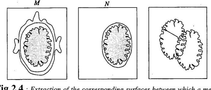
M N

Fig 2.4

: Extraction of the corresponding surfaces between which a measure o f mis

alignment may be derived.

Surface matching can be thought of as the problem of aligning two sets of points where

the one-to-one correspondence of pairing is unknown. Given a pair of point sets,

X = {xi} where i = 1,2,....K

Y = {yj} wherej = 1,2,....L (2.9)

describing surfaces X and Y respectively. Even if the surfaces exactly correspond, at registration the points on the surfaces are not necessarily aligned and, even the number of

points on the surfaces need not be the same. Because we do not have any point

correspondence information, we need, for a given point xi, a function for the transformation T

which returns a corresponding co-ordinate on the other surface described by the set Y, say

P(T(Y),xi). This may simply be the nearest point in the second set or a more complex description (for example a point on the triangulation of surface points Y). Given this function,

we can then develop a measure similar to that for point matching, based on the overall

distance between the surface.

Ds { T) =

I

Ell

X i - P ( T ( Y ) , Xi

1 = 7

(2.10)

The alignment by finding the value of T which minimises Ds(T) requires an iterative

search. The difference between point based alignment and surface based alignment is that

point based alignment is truly a measure of the distance from correct alignment of the two

corresponding point sets. Surface based alignment on the other hand, is not a direct ‘distance

to registration’ but, simply a measure of the alignment of the two surfaces.

S u r fa c e id e n tific a tio n a n d h a n d in g

(26)

the skin surface which is relatively easy to extract. The two problems posed by this are the

accuracy of rigid alignment estimates due to skin surface deformation, and the robustness of

the matching due to symmetries and lack of the fine structure in the skin surface. Some workers employ manually initiated extraction of the brain boundary from MR and SPECT and

PET where the skin surface extraction is more difficult. For MR-CT registration, skull

boundaries are extracted from MR for matching with those from CT by histogram

thresholding at 15% and 65% at the maximum MR value by one group [38]. Hill [39] was the

first to use neighbouring surface to derive a registration estimate. This work illustrated

registration using alignment of the inner skull surface extracted from CT and the outer brain

surface extracted from MR.

Handing outliners is another important aspect of matching surfaces. If the outliers in one

object are different from another, these could shift the correct optimum leading to error in alignment. One approach to this problem is to specifically exclude regions were differences

occur, but again this generally requires some form of manual intervention. Some groups

employed a simple form of thresholding, to exclude the influence of outliers, distances to nearest points were simply thresholded to a particular value chosen experimentally.

S u r fa c e m a tc h in g a p p r o a c h e s

Chen, Pelizzari, and co-workers, developed a popular 3-D parametric correspondence

method to register tomographic brain images. A surface module (head) extracted from one

image is related to a set of points (hat) extracted from contours in another image by a rigid and

optionally affine transformation [16]. The “hat” is fitted on the “head” by a search strategy

that uses a least squares fit. In order to make the task easier, the approach employs a number

of simplifications. The contribution to the residual for each “hat” point is evaluated by finding

the intersection with the “head” surface of a ray from the transformed “hat” point to the

centroid of the “head” model. This approach assumes, given the centroids are initially aligned,

that the two surfaces are predominantly spherical, so that the ray directions defined from the

centroid are close to the true nearest point direction. Sufficient surface should be scanned to

prevent the problem from being ill-posed. An accuracy of the order of one to two pixels of

the image with the lowest resolution has been achieved in phantom studies for CT, MR, and

PET.

This method has been used successfully at several clinical sites. The surface matching

technique is evaluated in the spatial correlation of SPECT and MR cardiac images [7]. The

method is based on matching corresponding anatomical surfaces extracted from transmission

SPECT and MR studies. Patients with brain tumours were studied on one or more occasions using MR and high resolution FDG-PET to analyse the brain tumour [18] [40]. PET-CT

(27)

The evaluation of the goodness-of-match function used by a parametric correspondence

method can be optimised for speed by applying a distance transform to the static image using

the “chamfering” method [38]. Rather than represent the two surfaces to be matched simply

by two lists of points, one of the objects delineated can be stored as a binary image where

voxels or pixel values are either object or background. From this binary image, a distance

image, can be formed using a ‘distance transform’ where each voxel or pixel outside the

object is given a value representing its distance to the nearest point on the object. To evaluate

the overall distance between two objects for a given transformation, the set of points

describing the object in one image is simply transformed to locations in the distance image of

the other object. The method has been used for SPECT- CT image registration [38].

2.2.3 C o m b in in g d iffe r e n t ty p e s o f g e o m e tr ic a l fe a tu r e

One of the major criticisms of feature based approaches is that they are using only a small part of information available in the images to determine image alignment. In many cases a

surface may not constrain the registration adequately or there may be inadequate numbers of

corresponding points in the images to provide an accurate estimate. Recently there has been considerable interest in using different types of geometrical features in determining 3D

alignment.

Pietrzyk, et al. [10] manually determined a 3-D transformation relating two tomographic

brain images. Aided by both separate and fused displays of multiple slices from the images to

be matched. Seitz et al. [11] used interactive methods for local curved matching of atlas

contours with patient images. Some methods solve a 3-D registration problem in two steps,

either of which may be interactive. Kapouleas et al. [13] first semi-automatically aligned the

mid-sagittal planes using indicated end points of the midline in all relevant axial MR and PET brain slices, then the remaining 2-D translation and rotation were determined manually by

aligning the overlaid outline of each sagittal MR slice on the corresponding resliced PET

image. Yaorong [14] described a registration method similar to that of Kapouleas et al. except

that, in the second step, equivalent points are identified by the user and the collection of paired

points from multiple parasagittal slices is registered using a simple least-squares minimisation

algorithm.

A number of approaches have been proposed to include structural information in the matching process, e.g., curves, planes [15] [17]. All methods reviewed based on structures use

intrinsic image properties and generate global approximating transformations: most methods

(28)

2.2.4 M o m e n ts/p rin cip a l a x e s m a tc h in g

A frequently used approach in image matching is based on moment matching techniques.

Volumes [20] and surfaces or scattered points [4] can all be used with moment matching.

From the moments of inertia, the principal axes of the object can be derived. Translation is

calculated from the position of the centroid of an object or a set of landmarks (equal to the

first order moments), and rotation is calculated by aligning the object’s or landmark

population’s principal axes of inertia (equal of the second order moments), which renders this

technique direct. Moments matching techniques produce approximating transformations

because they are based on statistical principles. Furthermore, as many points are needed, in

practice only intrinsic properties are used. Generally, the approach is semi-automatic as some

user interaction is needed to extract the image properties.

Moment matching techniques will result in inaccurate rotational parameters when,

because of symmetry, there are no unique principle axes. This absence seems more probable

with landmarks than with surfaces or volumes in medical applications. Differences in the scanned volume and large slice spacing may affect all parameters if a significant part of the

volume of the object is missing in one or both of the scans. The result may therefore be

unreliable in specific pathological cases, for example when matching functional images

showing peripheral metabolic deficiencies with images depicting anatomy.

2 .2 .5 I m a g e s i m i l a r i t y a s a m e a s u r e o f a l i g n m e n t

A similarity can be derived from the global relationship between voxel values in the two

modalities. The basic idea is that two values m and n are related or similar simply if there are

many other examples of those values occurring together in the overlapping imaged volume.

Effectively it can be said that in aligning the images the transformation is changed in order to

increase the clustering of the joint probability distribution so that there are few low probability

pairs and more higher probability pairs. In terms of the delineated regions, a transformation is

sought which maximises clustering for the volume of the majority of the interesting region.

We can express an overall image similarity S for a transformation T between the two images,

as the sum of individual measurement similarities S(.), at Q different points

Ô

S{ T) = Z 5 ( m ( X i ) , n ( T ( X i ) ) ) , ( 2 . 1 1 )

i = J

where m(xi) and n(T(xi)) are corresponding values. We would like 5 to be a monotonie

function of misalignment, which behaves like a mean distance between features. For this to be

the case, the number of pairs i=i S(.)) should fall smoothly with misalignment. We must

(29)

alignment. In many cases this is a valid assumption for many 3D medical modalities. The key

question in this approach is then how do we say whether values in the modalities are similar,

i.e. what do we use for our function S(.)7

Multi-modality imaging is the process of using measurements of different physical

properties to delineate different regions of material in the body. We can refer to a single

modality as providing a view of the underlying scene. It is the unknown relationship between

these views which forms the basic problem of multi-modality alignment.

In this case, unlike conventional computer vision problems, the view of the scene differs

not because of camera angle or the removal or introduction of objects, but simply because of

the difference in the property being imaged. A related field is that of multi-spectral remote

sensing, where it is conventional for images at different wavelengths to be acquired

simultaneously and therefore in correspondence. In medical imaging such an arrangement is unlikely to be feasible either technically or financially in a clinical setting.

We can image the scene with a device which will make measurements of a property at

points X E Vm. The device will record the actual underlying values m(x) as an image of

measurement m(x). Here a value falls within the set M of possible values and a measurement

within the set M of possible measurements. Examples of properties imaged for medical use are:

•X-ray linear attenuation coefficient p

•Radioisotope density resulting from tracer uptake in tissues

•Proton spin density and relaxation times

A scene may be divided into sets of points (which are termed regions) which exhibit a

particular value,

y/(m) = { X I X e Vm, m(x) = m} . (2.12)

The complete image consists of the set of regions delineated by each of the occurring

value m s M

M (M) = {k I k =i//(m), m e M } . (2.13)

The regions M are determined by the properties meM , of each of the anatomical or

physiological classifications reR summarised by the mapping,

(30)

If there exists a simple one-to-one mapping from classification of material to properties of

those materials, then we have an ideal modality which can delineate all the regions of interest

within the patient. In practice this is often not the case, and the imaged property does not

distinguish all the regions needed for a clinically sufficient description. Here there will be one

or more pairs of regions which exhibit the same values of the property so that the mapping is

not one-to-one.

As a result a second modality is often used to provide an image n{x) of a measurement of

a second property n e N, for which the mapping R - ^ N will be different. This new image

will then delineate a second set of regions N(N) as illustrated in Fig 2.5

A n ato m y /P h y sio lo g y P ro p erty M P ro p e rty N

Fig 2.5

Alternative ‘view ’ o f structure within a volume provided by measurement of

different properties.

A representation which captures the relationships between volumes of all regions

delineated by a pair of images is the joint histogram of values. For each pair of values of two

properties, the number of points at which those values occur together in the imaged volume of

overlap is recorded in a 2 dimensional array, resulting in a direct estimate of the matrix. By

normalising each volume by the total imaged volume of overlap,

V o (T ) = V (V m n T (V n )) we can form a joint probability distribution

P(M ,V ) = 1 U (T ). ( 2 .1 5 )

(31)

P(M , N) =

p { m i , n i } p { m i , n 2 } p { mi , r i j }

p{m2,ni}p{m2,ri2}

p{m2,rij}

p{mi,ni}p{mi,n2]

p[mi,rij}

(2.2 0)

represent the probability of occurrence of individual pairs of values in the images region.

From this we can extract the marginal probability distributions of the sets of values in

each view of the scene alone,

p{m} = ^ p{m, n } , ( 2 . 2 1 )

h gN

and

p{«} = X P ( ^ ' "}• ( 2. 2 2 )

m e M

S u m o f a b s o l u t e v a l u e d i f f e r e n c e (S A V D )

The simplest and most direct measure of similarity of two image values is given by their

absolute difference. An overall measure of alignment may then be determined by the average

absolute difference over each of the Q measurement points,

1 ^

S A V D ( T ) = - 2 1 1 m ( X i ) -n(T( X i ) ) (2.23)

i = l

In applying this measure we are assuming that the image values are effectively calibrated

to the same scale so that corresponding objects exhibit the same measurement value. If this is

the case then SAVD will tend to zero at alignment, if this is not the case then the behaviour is

less predictable, depending on the measurement values delineating the largest regions. It is

interesting to consider the amount of influence that a boundary between two regions has on

the overall measure for two transformations say T1 and T2 [43]. Equation 2.23 shows that it

will obviously depend on the difference of values across the boundary n(T7(Xi))-n(T2(Xi)). The

overall influence is dependent on the length and orientation of the boundary. The influence

though does not depend on the size of the objects at either side of the boundary. High contrast

boundaries between small objects may therefore have a greater influence on the measure than

(32)

SAVD is ideal in cases where two images are identical expect for noise. Example

applications include the alignment of images acquired to investigate the progression or

regression of disease, or changes in the chemical state in the brain. Application of this

approach to aligning other modalities where image values are not directly related is limited.

Even the simplest application of matching one MR image to another of the same sequence is

complicated by the varied scaling between two seemingly identical acquisitions.

This method has been used for SPECT and PET studies of phantoms and patients [43].

The technique is relatively unaffected by localised differences in activity distribution and the

range of noise in clinical studies.

C o r r e l a t i o n

In the simplest case of within modality registration, for example aligning two MR images

of the same sequence, registration results in a strong linear relationship between

corresponding values in two images. Misalignment then breaks down this relationship as

different values over-lie each other. In this case an obvious measure of similarity S(.) would

be one which determines a linear fit to the distribution of corresponding values. In deriving a

match from the fit of the data to a line of any gradient, we can avoid the problems of intensity

scaling experienced with the SAVD measure.

This approach is employed in the most commonly used measure of image alignment,

correlation, and is expressed simply as the sum of the product of all the pairs of values in the

images,

Q

y (T) = X m ( X i ) . « ( r ( x i ) ) ( 2 . 2 4 )

i = l

There are two basic limitations of this function when used as a measure of image

alignment. Firstly, it is not independent of the number of points over which it is evaluated. In

comparing two transformations, there may be significantly different regions of overlap

between the imaged volumes, and so appreciably different numbers of points Q available for

evaluation of y. In such a case the correlation would tend to be greater for the transformation

resulting in the greater volume of overlap. This can be avoided simply by dividing y by the

number of points,

f (T) = ^ ( 2 . 2 5 )

Q

(33)

Equation 2.25 is also not independent of the overall level of the signal in the region of overlap

and so the measure would tend to favour alignments which include larger image values. As a

result, a better measure of alignment of finite images is the Correlation Coefficient where we

consider the mean values of the two images over the set of Q points. Mathematically the

correlation coefficient is a measure of the residual errors from the fitting of a line to the data

by minimisation of least squares. In the field of signal processing the correlation of a signal

with a known signal is template matching. Matching filtering or convolution is simply the

correlation of a signal with a known signal reflected along each of its axes. Correlation would

be expected to be useful only for image types where the relationship between values in the

two images is predominantly linear at registration.

Correlation based methods map regions of pixels on a best-fit basis, and therefore are

approximating, and always search-based and intrinsic [21] [22]. Grey value correlation of

original pixel intensities is generally not useful for multimodality matching, as pixel

intensities in different modalities are usually not functions of correlating parameters.

V a r i a n c e o f i n t e n s i t y r a t i o

This is a simple statistical measure proposed by Woods [69] for aligning one PET image to another of the same patient. Empirically, when the pair of images are correctly aligned then

for each of corresponding values in the images, the ratio,

of their values is evaluated. The standard deviation of this ratio a r is evaluated over all i voxel

pairs. This is then normalised by dividing by the mean value r’ of each of the voxel pairs,

« = — ( 2 . 2 7 )

r'

giving a final measure of alignment which is minimised at registration. This is closely related

to the correlation coefficient and assumes that there is a constant scaling factor relating the

values in one image to the other at registration.

C o r r e s p o n d i n g i n t e n s i t y v a r i a n c e

Woods proposed the minimisation of corresponding variance for multi-modality

registration of MR and PET imagery of the brain. To align the images, the algorithm seeks to

minimise the standard deviation of the PET pixel values that correspond to each MR pixel

(34)

corresponding voxels in the second image n(T(x)), say Nm. Similarly we can find the standard

deviation of those values 6n(m). For a particular value m then we can work out the normalised standard deviation,

5n(m) = 6 n ( m )/ Nm. ( 2. 28)

The standard deviation of the distribution of intensities n for each intensity m should be

minimised at registration. Given a probability of occurrence for each value m, say p(m), a

weighted sum of the normalised standard deviation of the values N corresponding to each

MR value m e M ,

5(iV ) = X p (m) 6 ‘ n (m ). ( 2 . 2 9)

m e M

provides a measure of alignment. The weighting ensures that the measure is influenced most

strongly by PET intensity variation for the most common MR values.

The basic assumption this approach makes is that, at registration, uniform regions in one image map to uniform regions in the other. As the images move away from alignment,

measuring the spread of corresponding values by their variance gives a direct measure of

alignment. In practice this though may be approximately true for images where there are only

small differences.

If for two images at registration, one value maps to two significantly different values in

the other modality, then a measure of the clustering around the mean value will provide a poor

indication of alignment. The degree to which there is a direct one to one mapping between

values in the two images will determine the applicability of this measure. In order to ensure a

close to one-to-one mapping of values in his application. Woods employed a simple MR

segmentation to exclude non-brain regions, particularly scalp, from the measure.

What is also important is the direction of the mapping, i.e. choosing to minimise

corresponding variance in the first or second modality can make a significant difference. One

modality, say MR, may delineate significantly more regions than say PET and so every value

in the MR may map to only one value in the PET (expect perhaps a small region of

physiological abnormality), while the reverse is not true.

Imran [44] has used Woods method to assess the accuracy and reliability for standardization of brain SPECT images of patients with Alzheimer’s disease. There was

significantly decreased regional cerebral blood flow in the frontal, parietal, and temporal