Features of an electricity supply system based
on variable input
F. Wagner
Max-Planck-Institut f¨ur Plasmaphysik - Greifswald, Germany, EURATOM Association and Research Laboratory for Advanced Tokamak Physics
St. Petersburg State Polytechnic University - St. Petersburg, Russia
Summary.— In this paper we analyse and present the major features of electricity production being based predominantly on variable wind onshore and offshore and on photovoltaic generation. Actual data are taken from the German demand and supply situation in 2010. On this basis, the generation capacities are scaled to higher installed powers. The main purpose of the paper is to show characteristic trends and the mostly system oriented consequences of large-scale wind and solar use with fluctuating input.
1. – Introduction
The need and desire for energy will further grow because the Earth population will further grow and the per-capita energy use will continue increasing: A saturation of the population can only occur over decades; the increase in per-capita energy is driven by the large global differences in the individual availability of primary energy ranging from tens of kW to a few 100 W in terms of power. The success with new energy technologies will decide about the avoidance of societal frictions in possible periods of deficit and energy C
TableI. –Electricity sources in Germany in 2010[4].
Source TWh %
Coal 105.8 18
Lignite 135.2 23
Nuclear 135.2 23
Gas 82.3 14
Wind onshore 35.3 6
Photovoltaic 11.8 2
Bio-mass 29.4 5
Hydro electricity 17.6 3
Oil, pump storage, others 29.4 5
waste 5.9 1
paucity and the prevention of the ongoing environmental damages by the replacement of fossil fuels.
There are only three paths to a sustainable energy supply system — fission on the basis of breeders, fusion, and renewable energies (REs) in their different forms of occurrence [1]. In this paper we analyse the major characteristics of an electricity supply system which is predominantly based on RE. We do this with the example of Germany because of the rapid deployment of renewable energies. Germany will soon demonstrate the pros and cons of a rapid technology change for an essential commodity of the economy like electricity and it provides an attractive basis for a forward-looking analysis(1).
2. – Starting data of 2010
Modelling of characteristics of the electricity supply system for Germany with increas-ing contributions of the RE forms wind (on and offshore,WonandWoff) and photovoltaic (PV) power has been studied on the basis of available data of 2010. The 2010 data are publicly available for demand, onshore wind and PV. For offshore wind power, they had to be constructed from wind velocity measurement scaled to the offshore wind energy gained from the Alpha Ventus wind power park. The construction and details of the data set are described in the appendix.
In 2010, the net electricity production in Germany of 588 TWh originates from the different sources according to table I.
The fossil fuel fraction is about 55%. The 35.3 TWh from onshore wind were produced by 27.2 GW installed wind power and correspond to about 1300 h at full load (full load hours, flh, = harvested annual electrical energy/installed power) or, equivalently, to
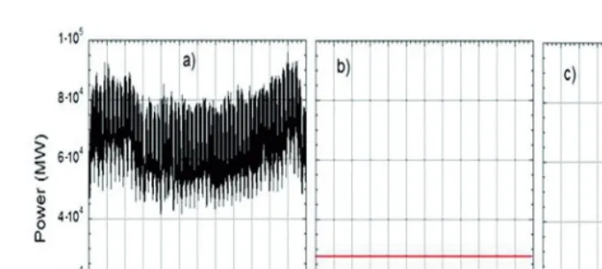
Fig. 1. – a) Variation of the load during 2010; b) onshore wind power in 2010; the red line denotes the installed wind power; c) PV power in 2010 but for constant installed power of 16.8 GW (red line) correcting the strong build-up of PV systems through the year.
a capacity factor (or availability factor, cf = flh/8760) in the use of the installations of 15% (2010 was a low-wind year). The up scaled 13.4 TWh from PV are based on 16.8 GW installed PV power and correspond to about 800 h of full load or to a capacity factor of 9%. The operation of the Alpha Ventus wind farm for a full year would have yielded 0.203 TWh for the 60 MW installed power. This corresponds to 3400 h at full load or a capacity factor of 39%.
Figures 1 a) to c) depict the data base constructed from actual data of 2010 as described in the appendix. Plotted are a) the demand (load), b) the onshore wind power and c) the PV power in their temporal developments through the year 2010. The PV data have been corrected for constant installed power. The horizontal lines in fig. 1 b) and c) represent the actually installed power levels, which are found to be larger than the power peaks in the data sets indicating a reduced average availability. Figure 1 shows both the weekly and the seasonal variation of the reduced load; the daily variation is not resolved.
Figure 2. plots the load, onshore wind, and, on top of it, the PV contributions for January and July 2010 from the data set of fig. 1 in more detail with the daily variation being resolved now. The demand is lower during the weekends; wind is erratic and larger in winter and spring. PV responds in a periodic form — clearly visible in July — with maxima coinciding with the load maxima around noon-time.
Fig. 2. – Load, onshore wind and, on top of it, PV are shown for January and July 2010.
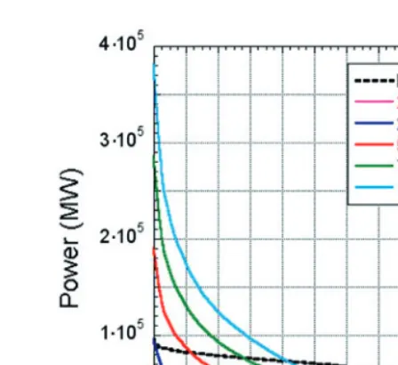
dubbed “reduced load” in this paper, is obtained when the electricity contributions from hydro, storage and waste are subtracted; curve 3 represents the load after wind and PV contributions are subtracted (residual load).
Curve 4 and 5 are the duration curves of wind and PV, respectively. The horizontal line and the area beneath denote the corresponding nuclear base-load contribution in 2010; the grey area corresponds to the production of fossil power stations with CO2 re-lease. Curve 4 shows that wind blows nearly throughout the year, whereas PV contributes for about half a year because of nighttimes without delivery.
Fig. 4. – Duration curves representing the load (black) and onshore wind electricity (in colour) of 2010 along with scaled up values representing up to 100% of the average annual electricity demand.
Figure 3 points to a fundamental problem in the use of RE. The load curve is — seen from above — largely convex. The duration curves of wind and PV, however, are concave. Scaling to higher levels of wind and PV power capacity in order to ultimately match the annual energy consumption leads to large energy surpluses for extended periods. Figure 4 illustrates this consequence of the different duration curve curvatures in an exemplary way for onshore wind scaled up to increasing shares of the annual electricity production. For the case that onshore wind delivers the same amount of energy as the load demands (100% curve in fig. 4) the areas beneath this curve and the one beneath the load curve are the same. The temporal distributions of available power and demand, however, do not fit. The area where the 100% curve is above the load represents the surplus energy; the area with the load being above the 100% curve has to be delivered additionally by a back-up system satisfying the residual load. This 100% case is denoted in this paper as the “equal energy case”.
Fig. 5. – For the conditions of the first week in February 2010 the load (black), directly dispatched RE power (blue) and surplus power (red) are plotted. The RE part is scaled such that the annual energy of load and RE are the same (“equal energy case”). Wind and PV are mixed in the form of the “optimal mix” as discussed in sect.4.
3. – Scaling studies
Whereas the net electricity production in 2010 is 588 TWh, the reference load value for the scaling studies of this paper is the “reduced load” of 562 TWh with the contributions from hydro, waste and storage electricity subtracted. We will not consider a bio-mass contribution assuming that the energy from bio-mass will be used in the future more for transportation, preferably for air traffic and less for electricity production. We further assume that the electricity consumption will not change expecting that effects of higher efficiency will be compensated by an expansion of the use of electricity e.g.in the field of mobility and smart supply systems or by technical measures, which will help reducing the primary energy consumption like a wide use of heat pumps. Nuclear energy and net electricity import are not considered.
For each time pointiin the data base the load, the on- and offshore wind power and the PV power are given. A positive difference between load and the sum of the three RE forms defines the back-up power at the time intervali. A negative difference (RE power >load) gives the surplus power.
Fig. 6. – a) The scaled RE power is plotted for the case that the annual electricity production by RE is equal to the annual demand. Black represents the directly dispatched power up to the load as upper limit; red (negative) the surplus power. a) Onshore wind, b) offshore wind and c) PV.
fig. 5 is constructed such that the annual energies of load and RE sources are the same — the so-called “equal energy case”. In this specific case the integral energies of the back-up system is equivalent to that of the surplus. The mix of RE energies in fig. 4 corresponds to the so-called “optimal mix” to be discussed in sect.4.
3.1.RE produce 100% of the annual electricity. – Each of the RE supply forms has its own characteristics. In order to elucidate these features we first analyse and discuss them separately. The RE power in these cases is selected such that for each form separately the RE produces as much energy as the load integrally demands. The intention with the termination at this point is that the surplus power — if proper storage were available — would just be sufficient to compensate the primarily missing energy. In this case, no back-up power would be required any longer. Transfer and other process losses are not considered here.
Figure 6 a) to c) represent the power of onshore and offshore wind and of PV. Positive values denote the power directly contributing to satisfy the demand. The upper limit of the curves is determined by the load. What goes beyond the load represents the surplus power and is plotted negatively.
– Onshore wind power fluctuates with large amplitudes truly reflecting the variability of wind velocity. Onshore turbines rarely meet the conditions of strong winds where the wind turbines are switched to the constant output power mode.
– Opposite to this, offshore wind power is rather constant in amplitude because strong wind leads to prolonged phases with the turbines regulated at the rated output power point.
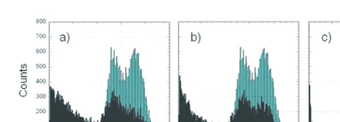
Fig. 7. – Histograms of the dispatched power (black) scaled to the 100% limit compared to the load of 2010 in each of the cases. a) Onshore wind; b) offshore wind; c) PV.
The two wind cases show lower power coverage of the load in summer whereas, recip-rocally, the low coverage by PV is in the winter months. The surplus power peaks can be exceedingly high in the limit considered here (“equal energy case”) and reach values frequently beyond 300 GW in case of PV and onshore wind.
The histograms in fig. 7 plot the directly used power (black) produced by the three RE forms, which is delivered into the grid. It is compared with the load (green). The load distribution is characterized by two maxima, the higher-power one representing rather the load during the day, the lower-power one the load more during the night and weekends. The width of the two profiles is mostly given by the seasonal cycle. The RE powers show typically the concave distribution with the frequency of occurrence decreasing toward higher powers. The distribution of the directly used power increases, however, in the power range of the load because all power values falling into this interval but also all higher ones contribute to it. Because of the decay of the distribution toward higher powers, the “filling” of the power band of the load requires a large installed power so that specifically the excess power levels can be used to fill the load power band, which is offset from zero by a gap — the base load. The selectiveness of this process is obvious from fig. 7 c). In case of PV, the highest peaks are delivered during daytime. Therefore, the day-peak of the load is preferentially filled.
Both onshore and offshore wind produce powers up to the level of the demand curve. But the highest power peaks of the load occur in winter during daytime with little PV contribution. Therefore, this part of the load is — unlike the other cases — not covered in case of PV; a gap remains between the peak load and the PV distribution at the highest powers. For these periods, when exclusively PV is considered, the back-up system must be available up to the maximal required power.
TableII. –The key characteristics of the three RE cases under the condition that the annual energy produced by the RE system is equal to the annual energy demand. The maximal power (identified as a lower limit to the installed power, because the average availability factor < 1, see fig.1), the directly used energy into the grid and the energy delivered by the back-up system which is equal to the surplus energy.
Maximal power Directly used energy Back-up = surplus energy
(GW) (TWh) (TWh)
Wind onshore 365 344 218
Wind offshore 165 344 218
PV 463 214 348
Table II shows the various key characteristics of the three RE forms under the limiting condition of the “equal energy case”.
For the same annual energy, the necessary wind power to be installed is lower by a factor of more than 2 in case of offshore than onshore wind. The energy values for directly used and surplus/back-up energies, respectively, are the same for the wind cases because of a similar data structure representative of turbulent generation processes; they are different for PV with a more periodic spectral content. In a control run with random numbers replacing actual wind or PV data, the directly used, surpluss, and back-up power levels are equal at 281 TWh adding up to the reduced load of 562 TWh.
Figure 8 a) to c) show the duration curves for the three cases considered. The black curve is the reduced load as defined above. The blue curves represent the RE power, which can directly be used. On- and offshore wind have contributions almost throughout the year. PV covers only about 50% of the year. The green curves denote the duration curve for the residual back-up power. Its contribution is strongly reduced compared to
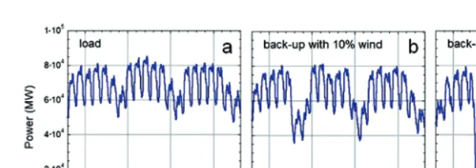
Fig. 9. – a) The load of the period from mid-February to mid-March 2010. Panels b) and c) represent the variation of the back-up systems when 10% or 30%, respectively, is contributed by onshore wind.
the original situation without RE contribution (see table II); it loses the characteristics of a base load. The negative red curves represent the surplus power reproducing the already known effect that the surplus power is limited in case of offshore wind and extreme in case of PV.
3.2. Surplus power and operation mode of the back-up system. – With controllable sources, the power supply system responds to the periodic variation of the day/night cycle, the weekly and the seasonal variation: Electricity production is demand driven. The load variations are periodic and rather predictable. With RE the supply system splits up into the primary sources wind and PV and the secondary source, the back-up system based on thermal power for the near future covering the residual load. With increasing RE shares, the periodic variation of the back-up systems is changed to an erratic one reflecting the spectral character of the stochastic supply and to a lesser extent the periodic pattern of the load: Electricity production becomes supply driven.
Figure 9 shows the variation of the back-up power with onshore wind energy shares increasing from 0 to 30% of the annual demands. With 10% wind contribution the periodic pattern of the load is largely maintained. This reflects roughly the 2011 situation in Germany (wind and PV: 66 TWh = 11% of the demand [2]). With 30% share, the periodic pattern is dissolved and the temporal characteristics of the residual power display chaotic traits.
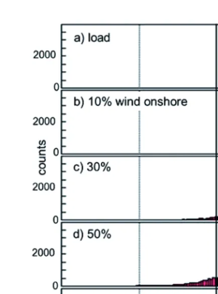
In the following, we discuss the features in the transition from continuous to variable supply along power histograms. Figure 10 a) shows the power histogram of the reduced load. The peak and the base load powers are shown as vertical lines. The double-hump structure has already been discussed.
Fig. 10. – Histograms of the load and the power delivered by back-up systems (black) and of the surplus power (red) with onshore wind contributions increasing from 10% to 100% of the annually demanded electricity in 2010. The vertical lines denote the base-load (blue) and the peak-load (red) levels.
annual electricity (fig. 10 c)), the base load has disappeared and the back-up system has to supply all power levels from 0 to the maxima of the reduced load. In this case, already a distinct amount of surplus electricity is produced, which is plotted on the negative axis (red). This trend continues to larger wind electricity shares (fig. 10d) with surplus power levels reaching beyond 100 GW. Figure 10 e) represents the case where the annually produced wind energy (sum of directly used and surplus energies) is equivalent to the annual demand (“equal energy case”). Figure 10e) also shows the small shift of the power range of the back-up system away from the original peak load line to a slightly lower value. For this case, close to 10% of the installed back-up capacity can be saved owing to the installed wind system and its continuous contribution throughout the year (see also table III).
TableIII. – Shown is the utilization of the back-up system (capacity factor) and its maximal power at variable RE contributions to the annual demand.
Energy source and RE contribution Capacity factor of Maximal power of
contribution (used+surplus) (%) back-up system back-up system (GW)
0 0.70 92
Wind onshore 10 0.67 86
Wind onshore 30 0.53 85
Wind onshore 50 0.43 84
Wind onshore 100 0.30 83
Wind offshore 100 0.29 87
PV 100 0.43 92
contributions of onshore wind and also for 100% energy from offshore wind or PV, re-spectively. For the “equal energy case” onshore and offshore wind reduces the back-up capacity factors to about 30%. In case of PV, the back-up system is more frequently in use. As already shown in fig. 7, PV does not allow a reduction in installed back-up power — unlike wind electricity with a reduction from 92 to 83 GW (−8%). The jump from 92 GW installed power to 86 GW with already 10% onshore wind is caused by the removal of peak load demands from the back-up system, which happens for about 50 h in the year. This effect may be a particularity of the wind situation in 2010.
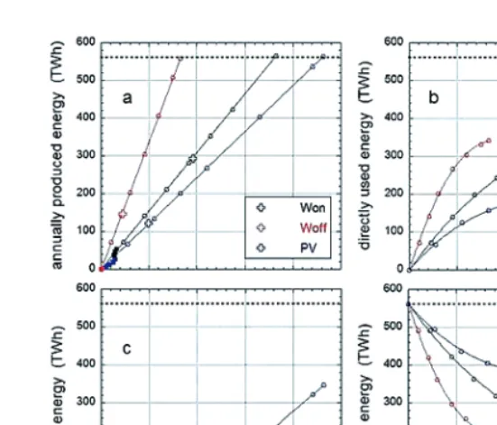
3.3.Summary of scaling studies. – In fig. 11 a) the produced RE electricity (directly used and surplus) is plotted against the maximal RE power in the data set of the re-spective scan for on- and offshore wind and PV. The relation is linear(2). Technical losses in production or transmission are neglected because they are not relevant for the considerations of this paper. The necessary installed power capacities are actually larger than the power values quoted here(3) by a factor of 1.2 for onshore wind or 1.5 for PV, respectively. For the truly installed power and the corresponding capital costs for their implementation, the maximal power values of fig. 11 represent therefore lower limits.
The horizontal dotted line in fig. 11 a) corresponds to the reduced load of integrally 562 TWh, which has to be produced to meet the 588 TWh net electricity target together with electricity from hydro and waste. The solid data points close to the origin represent energy and installed power of onshore wind (black squares), offshore wind (red square), and PV (blue square) at the end of 2010, and 2011 and as expected for 2012. These
(2) In reality, the relation is not linear rather bands over because in the process of increasing the installed power, less favorable locations have to be selected for RE production.
Fig. 11. – a) The produced energy against the maximal RE power in the data set (lower limit of the installed power) for on- and offshore wind and PV. The horizontal line represents the level of the reduced load in Germany in 2010. The squares close to the origin represent energy and installed power of onshore wind (black), offshore wind (red) and PV (blue) for 2010, 2011, and as expected for 2012. The open crosses represent the key data of the optimal mix of the RE system as described in sect. 4. b) directly used energy; c) surplus energy; d) back-up energy. The curves end when the total energy delivered by the RE systems is equal to the annual demand (see a)).
data points indicate the still infant nature of the RE deployment in Germany in spite of tremendous efforts. The open crosses indicate the locations of the three RE components in case of the optimal mix as described in sect. 4. All curves in fig. 11 end when the energy produced by RE agrees with the annual demand — at the conditions of the “equal energy case” (e.g., see fig. 11a)).
Figure 11 b) plots the annually produced energy, which is directly used for the three systems under consideration against the maximal power occurring in the data base. Figure 11 c) shows the annual surplus energy and finally, in fig. 11 d) the energy of the back-up system is plotted.
The directly used energy of fig. 11 b) shows the tendency to saturate. This effect is specifically distinct for PV. The non-linear elements causing the saturation are the periods without RE electricity production irrespective of the installed power — wind velocity below the cut-in level or the nights in case of PV. All of the three RE forms stay well below the reduced load (dotted line in fig. 11) for the conditions considered here.
Owing to their concave power spectrum (e.g. see fig. 4) RE systems produce large amounts of excess power (see fig. 11 c), which cannot be accommodated within the national grid without storage. PV produces the largest amount of surplus power.
The energy delivered by the back-up system for the three RE cases considered deceases with increasing RE share (see fig. 11d). This dependence corresponds to the desired objectives in the use of RE. Back-up power is required up to the “equal energy case” and beyond. An exclusive PV system would necessitate the largest thermal power back-up system.
In conclusion, without storage, offshore wind as the “best” RE electricity source pro-duces about 50% of the annual load with about twice the presently installed conventional thermal power. The other extreme is PV, which produces with close to 500 GW installed power only about 1/3 of the annual electricity.
4. – Optimal mix between wind and PV installations
The averaged load curve has a maximum in winter and a minimum in summer. This is also the case for wind electricity, which helps to match the seasonal cycle and is contrary to photovoltaic electricity production, which has a minimum in winter (see fig. 1). On the other hand, photovoltaic electricity is produced during the day when the demand is highest. Therefore, wind has a good annual and PV a good daily match to the load curve. The consequence is that there is an optimal mix for these two renewable energy forms. We define the optimum as the proper mix of wind and PV power, which minimizes the demand of back-up power (and therefore the amount of CO2 production as long as the back-up system is based on fossil fuels). We further assume that offshore wind produces 1/3 of the wind energy.
Figure 12 plots the annually produced energy of the back-up systems normalized to the reduced load against the PV energy production also normalized to the reduced load. Parameter of the set of curves is the total contribution of RE also normalized to the reduced load. The curves show a minimum, which moves to larger PV contributions when the share of RE increases. The curves do not represent a symmetric case for wind and PV. The wind-only case is not much above the minimum whereas the PV-only case requires much more back-up contributions.
Fig. 12. – The ratio of the back-up energy to the annual reduced electricity demand is plotted against the energy contribution of the PV system, also normalized to the reduced load. The parameter of the curves is the ratio of the energy delivered by the RE normalized against the reduced load. The offshore wind energy is assumed to be 1/3 of the total wind contribution.
Table IV shows the key parameters for the case that RE matches the reduced annual electricity production (562 TWh) under the optimized conditions of minimal back-up need. Onshore wind produces 2/3 of the total wind production in the case considered. Given is the power of each of the systems along with the energy it produces. As the REs do not match the load for each of the time points, 153 TWh have to be delivered by the back-up system (being equal to the surplus energy). The necessary installed power for this purpose is 84 GW.
TableIV. –Key data for the case that the RE systems produce under the optimal mix conditions
the amount of energy corresponding to the demand(“equal energy case”).
Power (GW) Energy (TWh)
Wind onshore 191 294
Wind offshore 44 147
PV 99 121
Back-up system 84 153
Surplus 153
Fig. 13. – The various energies involved and the maximal grid powerversus the annual energy from renewable sources normalized to the annual demand (RE share) for the optimal mix case.
Figure 13 shows the energies involved in meeting the annual demand — the one produced by RE, the directly used one, the surplus energy, and the residual energy of the back-up system. Shown is also the maximal grid power. The results are obtained under optimal mix conditions. The directly used RE energy (dark blue curve) increases non-linearly indicating — like in fig. 11 b) for the individual supply techniques — that RE as considered here will not meet the demand completely. The red curve in fig. 13 represents the surplus power. Surplus power starts playing a role beyond about 40% of RE share. The dotted curve is the dispatched power. The maximal power into the grid is 260 GW and is determined by the RE alone. The loading of the grid by the back-up systems does, of course, not affect its maximal loading capacity. The back-up power, which is not plotted, decreases slightly from 92 GW to 84 GW for the “equal energy case” — an 8% reduction in installed thermal power capacity. At an installed RE power equal to that of the back-up system (equal to the presently installed power system), the RE deliver 25–30% of the annual demand. A distinct difference in supply characteristics happens for RE shares>40% with a pronounced increase in surplus energy and in the power to the grid.
The crosses plotted in fig. 11 a) represent the key data in RE power and energy for the optimal mix case.
Fig. 14. – Capacity factor against the RE energy share for the back-up system.
The optimal mix case is not suggested here as a development scenario. This is not possible under the present deployment strategy in Germany and may not be possible at all. It rather serves as a reference case to assess and qualify alternatives.
5. – Temporal characteristics of power loading to the grid
The historic situation is characterized by power delivery by demand with controllable power plants categorized in base, medium and peak loads. The dynamics of the power system was determined by the periodic and rather predictable variation of the load. With increasing stochastic contributions both amplitude and response change and are now governed by the temporal characteristics of the fluctuating sources (see fig. 9). A detailed account of the consequences on the conventional power plants in Germany is given in ref. [3].
Fig. 15. – Histogram of the power levels for the “equal energy case” with on- and offshore wind, PV and for the conditions of the “optimal mix case”.
We have seen that with increasing RE share the capacity factor of the back-up system drops. The periods become longer where the back-up system is not in operation. It can be expected that the number of power cycles for the back-up system therefore decreases with increasing RE contribution. The number of cycles above 1 GW power increment is plotted in fig. 16 for onshore wind with different shares and for offshore wind, PV and the optimal mix case for the 100% “equal energy case”. The cases|ΔP|<GW are excluded to separate the frequent small power steps from the critical excursions of interest here.
The distribution between positive and negative power increments is rather symmetric. As expected, the number of power switches drops toward high fractions of onshore wind. The maximum is at about an onshore power fraction of 60% with nearly 14000 bipolar large power cycles in a year. This goes nearly a factor of two beyond the number of equivalent cycles of the load. The consequence is a much stronger operational demand for the back-up system and represents a challenge to its technical integrity specifically for the larger power excursions necessitating a nearly coherent response of the back-up system. Some of the technical consequences are analysed in ref. [4].
6. – Storage
Storage would allow to use the surplus power and to ultimately replace the thermal technology of the back-up system achieving thus completely CO2-free electricity supply and would allow smoothing the fluctuations on RE electricity production. No specific storage technology is assumed here.
Fig. 16. – The number of power switches of the back-up system>1 GW are plotted against the annual RE normalized against the annual demand. The results for both positive and negative excursions are shown. For onshore wind, the continuous development from 0 to 100% RE contribution to the load is plotted; for the other cases (offshore, PV and the optimal mix case) only the results of the 100% (“equal energy”) cases are given. The solid curve is a guide to the eye for positive and the dashed curve for negativeWonpower increments.
parameters are developed first from the characteristics of the three types of sources assumed — on- and offshore wind or PV, respectively. At first, we discuss each source type separately. A condition for a long-term storage system is that its variation is periodic. As we consider one year, the storage conditions at the end of the year have to be the same as at the beginning. Under idealized model assumptions, we fix the initial storage level so that during the year, the complete storage capacity will be used.
Figure 17 shows the variation of the storage level over the year separately for onshore and offshore wind and PV. The “equal energy case” is considered because in this case the surplus energy (to be stored) equals the back-up energy (to be substituted). For the wind cases, the storage level has the tendency to increase in the first months of the year. The storage minimum is reached in August. For PV a larger storage has to be provided because it first empties in the first months till the minimum is reached in mid-March. In the months following March the storage steadily fills with the filling maximum in September-October. The PV storage follows a sinusoidal curve like the solar radiation, however 90◦ out of phase.
Fig. 17. – The variation of the storage loading with time through the year for the 4 cases considered.
Table V summarises the key parameters of the long-term storage system. PV requires by far the largest storage. Again, the benefit of the optimal mix is evident requiring the smallest capacity. The seasonal differences in input add up rather favourably in this case and reduce the size of storage. The maximal discharging power values (negative) are rather similar for the four cases and they are at the level of the back-up system to be replaced. The charging power levels (positive) are high and vary strongly, depending on the type of source. The maximal power is required, however, for shorter periods only. The figures in brackets in table V denote the periods where the power is above 100 GW. The smallest seasonal storage with a capacity of 33 TWh — as required for the optimal mix case — surpasses the one presently available in Germany by a factor of 500. Such a storage cannot be realised irrespective of the technology employed. Seasonal storage in a closed German system does not seem possible.
TableV. –Storage capacity and maximal storage power for the 4cases considered under the
conditions of the “equal energy/optimal mix case”; positive: charging; negative: dispatching; see fig.17. The respective period for the power>100 GWis given in brackets.
Storage energy (TWh) Maximal storage power (GW)
Onshore wind 60 +296,−83 (1 month)
Offshore wind 67 +123,−87 (24 days)
PV 166 +397,−92 (two months)
Fig. 18. – For the period shown, the needed back-up power is plotted without storage for the standard “equal energy/optimal mix case”. The negative values show the storage power for two cases, which differ in storage capacity, 2000 and 5000 GWh, respectively. The right ordinate shows the storage loading for the two capacities considered (lower traces).
6.2.Short-term storage. – In the following we investigate continuous operation of the storage — loading whenever surplus power is available up to a specified storage capacity and discharging whenever the RE delivery is insufficient till the storage is empty or a reloading period starts. Figure 18 shows for the period Jan. 23 till Feb. 13 first the time traces of the back-up power in a system without storage and then the storage power (plotted negatively) for two storage capacities — 2 and 5 TWh. Considered again is the “equal-energy case”. Also, the storage loadings (lower curves) are shown. This diagram serves to elucidate the operation of the storage and its impact on the dynamics of the back-up power system. When the storage is sufficiently filled, the power from the storage matches (and substitutes) the back-up power. The larger the storage capacity, the shorter are the remaining periods needing back-up support. When the storage is empty its power becomes zero and this happens for the larger capacity storage at a later time. When the storage is full, surplus power is not fully used and available for other means.
Fig. 19. – For one week in summer (a) and one in winter (b) the reduced load is shown for the standard “equal energy case” along with the power of the RE, the surplus energy, the power from charging (negative) and discharging the 200 GWh storage.
Discharging of the storage is erratic and is interrupted for longer periods in phases of large RE power with sufficient surplus production at a full storage or in periods of an empty storage without surplus production. The necessary back-up energy reduces from annually 153 TWh to 128 TWh in this case whereas the back-up power does not change. Figure 20 shows the duration curve, now of the storage system of different capacities starting from the reduced load and the residual load without storage in the limit of
TableVI. – The full-load hours(flh) and the capacity factors for storage and back-up system for the cases plotted in fig.20.
Storage capacity flh storage Capacity factor storage flh back-up system Capacity factor
(GWh) (h) (h) back-up system
50 177 0.02 1711 0.195
100 241 0.027 1636 0.187
500 541 0.062 1343 0.153
1000 768 0.088 1140 0.130
2000 957 0.109 899 0.103
5000 1244 0.142 603 0.069
the “equal energy/optimal mix case”. The positive branches show the discharging, the negative ones the charging periods. At low capacity, the charging periods are slightly longer than the discharging ones. This turns around for large storage capacities, which are able to accommodate large power peaks shortening the charging periods.
Table VI describes the use of storage and that of the back-up system in terms of full-load hours or capacity factors, respectively. These values address the question of economic use of the infrastructure. Full-load hours and capacity factors increase with storage capacity whereas those of the back-up system decrease. For the full range of storage capacity assumed the economic operation of storage and back-up system can be questioned. The lowest storage capacity of 50 GWh corresponds to the one presently available in Germany. This storage operates under economic conditions predominantly used to meet peak-load conditions. Here, however, we consider exclusively the conditions for surplus power storage.
The simplest, however uneconomic way to avoid surplus power is to stop dispatching RE into the grid. This may be technically more easily possible with wind converters than with PV systems. We consider the “equal energy, optimal mix case”. The sequence of interventions starts with reducing onshore wind power and continues — if necessary — via offshore wind to PV. If surplus power is available, first onshore wind is correspondingly reduced. If this is not sufficient, offshore wind is also reduced. The full-load hours of onshore wind drop from 1545 h to 828 h, those of offshore drop from 3385 h to 3117 h whereas there is no need to also reduce PV — which represents anyway the technically most complex form of intervention. As a consequence the peak onshore wind power values >100 GW are avoided; the system use is, however, practically halved with corresponding economic consequences.
7. – Scenario characteristics of a probable upper limit: 40% energy from RE sources
TableVII. –Key-parameters describing the power(GW)and annual energy values for the case that40% of the annual electricity demand are covered by RE under optimal mix conditions. The increase with respect to the situation in 2011 is also given. The values in brackets include the cor-rection of the maximal power values in the data base to the actually installed powers(see fig.1).
Technlogy Installed Annually Increase/decrease flh
power produced energy in power compared (h)
(GW) (TWh) to 2011
Reduced load 91 562 6116
Onshore wind 69 (82) 106 ×2.4 (2.8) 1545
Offshore wind 16 53 × ∼80 3384
PV 55 (84) 66 ×2.2 (3.4) 1217
Back-up system 86 340 −5.5% 3974
Surplus power 35 3
Storage 35 (charging) 2.7 77
Storage 47 (discharging) ×7.3
Maximal grid power 101
reasons for limitations — technical problems like grid stability or conflicting technical solutions like in Denmark between prioritized RE feed-in and CHP production by thermal power stations [5]. Here we assume that the limitations are given by an excessive level of surplus power and the short-term power increments, which can still be handled by the size of the storage needed, by the need to operate a back-up system economically and by the option to limit grid expansion capacity because of costs and its inherent societal complexity. Within these limits, we assume that RE can deliver 40% of the annual energy demand (see also fig. 13) and that Germany has available a storage capacity of 200 GWh. The key-data of such an electricity infrastructure are given in table VII.
8. – Analysis and comments
The production of electricity with variable sources is not the problem. If a soci-ety agrees to the corresponding use of land and finances the necessary investments the electricity to be produced can be increased proportional to the allocated area(4).
The following actual problems and issues in the large-scale use of RE have been identified:
– RE requires large power installations. The necessary investments can be reduced by a proper mix of wind and PV power. For the “optimal mix, equal energy” case, the energy, which has to be delivered by the back-up system and the associated CO2output are minimized. 84 GW installed power contributes with 153 GWh.
With the assumption of this paper (no electricity import, no use of bio-mass apart from waste), variable sources cannot meet the electricity demand alone. By increas-ing their share, the directly used power saturates well below the demand whereas the surplus power rises steeply.
Already at lower RE shares, close to and above 40% of the energy demand, the surplus power reaches a level, which can be handled neither by reasonable technol-ogy nor by cross-border trade. It also cannot be simply wasted because of its high economic value. The systems — preferably wind turbines — have to be throttled in this case accepting economic losses. Germany, though leading in the installation of RE systems, is still below any of these critical limits (see fig. 12 a).
PV is the most ineffective RE supply form. It requires the largest installed power per delivered energy unit and it causes extreme surplus power peaks. This negative aspect adds to those, which are well known and documented: PV has the highest material use, the highest primary energy use and the highest costs per unit of electricity produced [6].
– Without proper storage, the RE use cannot prevent the need for a back-up system of conventional power plants. The nominal power of the back-up system has to remain high and is hardly reduced by the addition of RE power. Its energy supply, however, which is the economic factor, decreases with increasing RE share.
The back-up system has to be operated under strongly varying conditions. The number of thermal cycles increases because the system dynamics is no longer de-termined by that of the demand rather by that of the supply.
– Large storage capacity both in energy and power handling capability is necessary replacing the back-up system of thermal power stations and thus optimizing the
CO2balance. A notable effect on reducing the size of the back-up supply requires a storage, which is far beyond any chances of realization.
– The use of variable sources with short full-load hours forces the other components of the supply system operated during the gaps also to low-capacity factors. Specif-ically, the increase in power installation causes a corresponding decrease of the full-load hours of the back-up system. The storage, when seen exclusively as a means to store surplus power, is subject to the same shortcomings causing low-capacity factors. The complete supply system comprises of components, which are not operated adequately in an economic sense.
Some of these issues are ameliorated by supra-national girds because both load and variable production are smoothed. It can be doubted that this will happen in near future. Energy policies in Europe are considered national sovereignty. Also the enforced deployment of RE in Germany, which — when continued with the present development speed — will produce tremendous amounts of surplus, will limit the expansion options of its neighbours because most conspicuously, surplus will be further increased.
As a consequence, the development of alternative electricity supply forms is still of highest relevance and may become even more urgent after a realistic view into the ca-pabilities and the limits of REs. Because of the limitations and shortcomings in their use, the most obvious question will be whether and how an electricity system based on variable sources can be improved and supplemented. This will be a question classically posed to research and engineering because these disciplines have found the ways in the past to liberate mankind from the imponderabilities and perils of nature.
∗ ∗ ∗
The author is grateful to his colleagues from the Board of the Energy Group of the European Physical Society for stimulating discussions. The clearance of the FINO data by the BMU and the Projekttr¨ager J¨ulich is gratefully acknowledged.
AppendixA.
Construction of the data set The following source data were used.
The electricity demand (load) was obtained from Tennet [7] with 15 min resolution and from ENTSO-E [8] with 1 h resolution. The more representative ENTSO-E data were taken. The ENTSO-E data were scaled to deliver the net electricity production of 588 TWh in 2010 (see table I) [9]. Thus, the demands both from the high-voltage and the lower-voltage grids are included.
The correlation coefficient R= 0.48. The correlation function has a distinct maximum with a delay of 2 h.
Offshore wind is not yet available in Germany to the extent that one could apply the same procedure as for onshore wind. The offshore data used were constructed from wind velocity data vw obtained from FINO3 [12]. Data were taken from the sensor at 100 m height pointing in 345◦ direction(5). The offshore wind power is given by the cubic relation: P =αvw3. In order to get verified power values the data from the first successful operation of the north-sea test-field Alpha Ventus wind park [13] were used. The 2×6 wind turbines with a nominal power of 5 MW each worked from October 2010 to June 2011 without interruption and produced 190 GWh. For the determination of α the wind velocity data were matched to the operational conditions of the wind turbines. The power was set to 0 for wind velocities vw <3.5 m/s (cut-in velocity) or vw > 30 m/s (which was not reached in the considered data sample); P was assumed to scale according to the above cubic relation between 3.5 m/s and 14.5 m/s and to be constant at the maximal power (5 MW) for 14.5 (rated velocity) < vw < 30 m/s (cut-out velocity). It is problematic to take point data as representatives for a turbulent field where, in the area, specifically the peaks average out to a certain extent. In case of offshore wind, the peaks are removed by the maximal power setting of the turbines. Therefore, this way of constructing the data seems justified.
Again, as a means of control, the FINO3 velocity data and the onshore wind power values were correlated (vw3 withPon). The correlation coefficient R= 0.46 indicating a weak but distinct relationship of the data as can be expected facing the long-range nature of the wind pattern over Germany (50Hertz region) and the German Bay region. The correlation is between a point value (FINO3 velocity) and a field average value (Pon). The correlation function has a maximum and decreases for larger time shifts between the data. For comparison, the offshore wind data were also correlated to the PV data. Of course, no correlation is expected. The correlation coefficient is found to beR= 0.09.
The photovoltaic data were obtained from 50Hertz in 15 min increments [10]. Like in the other cases, they were scaled to the photovoltaic energy harvested in 2010 of 11.8 TWh. A further correction was necessary because of the strong development of PV systems in Germany in 2010 growing from 9.9 GW installed power at the end of 2009 to 16.8 GW (up to 17.3 GW can be found in the literature) a year later. As we assume constant installed PV power for the scenarios to be analysed in this study, the 2010 data were corrected assuming a linear growth of installed power in 2010 (which differs from the actual growth curve, which is ignored). The corrected PV data set would have delivered 13.4 TWh at a constant installed power of 16.8 GW.
In this manner, a data base for the load,Won,Woffand PV power is obtained for 35040 time points with a resolution of 15 min. The ENTSO-E load data with 1 h time steps are kept constant over the 15 min time grid. The comparison with the regionally limited Tennet load data with 15 min resolution shows that no significant error is introduced by smoothing the load. Anyway, the major dynamics in the data base is introduced by the RE supply forms. For the temporal response studies of sect.5, however, the better time-resolved Tennet data were used.
REFERENCES
[1] For a general readership the book “Energy Survival Guide” by Jo Hermans gives a short but still broad introduction into many energy-related issues; “Sustainable Energy – without the hot air” by MacKaye is highly recommended for an interested readership specifically as it is also available at the internet (http://www.withouthotair.com/); specialised interests are best served by the Landolt-B¨ornstein series on Energy Technologies, volumes VIII/3A, B, and C. As we concentrate on wind and photovoltaic energies, the reader may turn to “Introduction to Wind Energy Systems” by H.-J. Wagner and J. Mathur and to “Physics of Solar Cells” by P. W¨urfel introducing into the physics background of these technologies. A general overview over the German electricity supply is provided by the study of the “Arbeitskreis Energie” of the German Physical Society: “Electricity: The key to a sustainable and climatecompatible energy system”: www.dpg-physik.de/ veroeffentlichung/broschueren/studien/energy 2011.pdf.
[2] www.ise.fraunhofer.de.
[3] Ziems Ch.et al., “Effects of fluctuating wind power and photovoltaic production to the
controlability and thermodynamic behaviour of conventional power plants in Germany”. VGB PowerTech Study, Uni Rostock.
[4] Weber H. et al., “Technical Framework Conditions to Integrate High Intermittent
Renewable Energy Feed-in in Germany”, Wind Energy Management, ISBN: 978-953-307-336-1, InTech, 2011. Available from: http://www.intechopen.com/books/windenergy- management/technical-framework-conditions-to-integrate-high-intermittent-renewable-energy-feed-inin-germany.
[5] Sharman H., “Wind Energy – the case of Denmark”, CEPOS, Sept. 2009 (www.cepos.dk).
[6] Marheineke T., “Lebenszyklusanalyse fossiler, nuklearer und regenerativer
Stromerzeugungstechniken”, IER Forschungsbericht, Band 87, 2002. [7] www.tennettso.de/site/Transparenz/veroeffentlichungen. [8] www.entsoe-eu.
[9] www.bmwi.de. [10] www.50hertz.com.
[11] www.transnetbw.de/kennzahlen/erneuerbare-energien/windeinspeisung/. [12] www.fino-offshore.de.