ISSN 0249-6399
ISRN INRIA/RR--4730--FR+ENG
a p p o r t
d e r e c h e r c h e
Survey: Probabilistic Methodology and Techniques
for Artefact Conception and Development
Pierre Bessière & the BIBA - INRIA Research Group
1- Projet CYBERMOVE
No
4 7 3 0
Févr
ier 2003
TH `EME3
Survey: Probabilistic Methodology and Techniques
for Artefact Conception and Development
Pierre Bessière & the BIBA - INRIA Research Group
1Projet CYBERMOVE
Thème 3 : Interaction homme-machine, images, données, connaissances
Rapport de recherche n°4730 - février 2003
Abstract: The purpose of this paper is to make a state of the art on probabilistic methodology and tech-niques for artefact conception and development. It is the 8th deliverable of the BIBA (Bayesian Inspired Brain and Artefacts) project. We first present the incompletness problem as the central diffi-culty that both living creatures and artefacts have to face: how can they perceive, infer, decide and act efficiently with incomplete and uncertain knowledge?. We then introduce a generic probabilistic formalism called Bayesian Programming. This formalism is then used to review the main probabilistic methodology and techniques. This review is organized in 3 parts: first the probabilistic models from Bayesian networks to Kalman filters and from sensor fusion to CAD systems, second the inference techniques and finally the learning and model acquisition and comparison methodologies. We conclude with the perspectives of the BIBA project as they rise from this state of the art.
Keywords: Bayesian programming, Bayesian modelling, Bayesian reasoning, Bayesian learning, Bayesian networks
2 Bessière et al.
Résumé : L’objectif de cet article est d’établir un état de l’art sur la méthodologie et les techniques probabilistes pour la conception et le développement d’artefacts. C’est le 8ème élément du projet BIBA (Bayesian Inspired Brain and Artefacts). Nous présentons tout d’abord le problème de l’incomplétude comme difficulté centrale à laquelle les êtres vivants et les artefacts doivent faire face : comment peuvent-ils percevoir, inférer, décider et agir efficacement avec une connaissance incomplète et incertaine?. Nous présentons ensuite un formalisme probabiliste générique appelé programmation bayésienne. Ce formalisme est utilisé pour examiner les principales méthodologie et techniques probabilistes. Cet état de l’art est organisé suivant 3 parties : premièrement les modèles probabilistes des réseaux bayésiens jusqu’aux filtres de Kalman et de la fusion de capteurs aux modèles CAO, deuxièmement les techniques d’inférence et finalement les méthodes de comparaison, d’acquisition et d’apprentissage. Nous con-cluons avec les perspectives du projet BIBA qui découlent de cet état de l’art.
Probalistic Methodology and Techniques for Artefact Conception and Development 3
1. I
NCOMPLETENESSANDU
NCERTAINTYWe think that over the next decade, probabilistic reasoning will provide a new paradigm for understanding neural mechanisms and the strategies of animal behaviour at a theoretical level, and will raise the perfor-mance of engineering artefacts to a point where they are no longer easily outperformed by the biological examples they are imitating.
The BIBA project has been motivated by this conviction and aims to advance in this direction. We assume that both living creatures and artefacts have to face the same fundamental difficulty:
incompleteness (and its direct consequence uncertainty). Any model of a real phenomenon is incomplete:
there are always some hidden variables, not taken into account in the model, that influence the phenome-non. The effect of these hidden variables is that the model and the phenomenon never behave exactly alike. Both living organisms and robotic systems must face this central difficulty: how to use an incom-plete model of their environment to perceive, infer, decide and act efficiently?
Rational reasoning with incomplete information is quite a challenge for artificial systems. The pur-pose of probabilistic inference and learning is precisely to tackle this problem with a well-established for-mal theory. During the past years a lot of progress has been made in this field both from the theoretical and applied point of view. The purpose of this paper is to give an overview of these works and especially to try a synthetic presentation using a generic formalism named Bayesian Programming (BP) to present all of them. It is not an impartial presentation of this field. Indeed, we present our own subjective "subjec-tivist" point of view and we think that is why it may be interesting.
The paper, after discussing further the incompleteness and uncertainty problems and how probabilis-tic reasoning helps deal with them, is organised in 4 main parts. The first part is a short and formal presen-tation of BP. The second part is a presenpresen-tation of the main probabilistic models found in the literature. The third part describes the principal techniques and algorithms for probabilistic inference. Finally, the fourth deals with the learning aspects.
1.1 Incompleteness and uncertainty in robotics
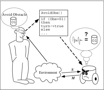
The dominant paradigm in robotics may be caricatured by Figure 1.
The programmer of the robot has an abstract conception of its environment. He or she can describe the environment in geometrical terms because the shape of objects and the map of the world can be
speci-Figure 1: The symbolic approach in robotics.
=
?
if (Obs=01)
then
turn:=true
else
...
AvoidObs()
Environment
O1
S
M
O1
4 Bessière et al.
fied. He or she may describe the environment in analytical terms because the laws of physics that govern this world are known. The environment may also be described in symbolic terms because both the objects and their characteristics can be named.
The programmer uses this abstract representation to program the robot. The programs use these geo-metric, analytic and symbolic notions. In a way, the programmer imposes on the robot his or her own abstract conception of the environment.
The difficulties of this approach appear when the robot needs to link these abstract concepts with the raw signals it obtains from its sensors and sends to its actuators.
The central origin of these difficulties is the irreducible incompleteness of the models. Indeed, there are always some hidden variables, not taken into account in the model, that influence the phenomenon. The effect of these hidden variables is that the model and the phenomenon never behave exactly the same. The hidden variables prevent the robot from relating the abstract concepts and the raw sensory-motor data reliably. The sensory-motor data are then said to be «noisy» or even «aberrant». An odd reversal of causal-ity occurs that seem to consider that the mathematical model is exact and that the physical world has some unknown flaws.
Controlling the environment is the usual answer to these difficulties. The programmer of the robot looks for the causes of «noises» and modifies either the robot or the environment to suppress these «flaws». The environment is modified until it corresponds to its mathematical model. This approach is both legitimate and efficient from an engineering point of view. A precise control of both the environment and the tasks ensures that industrial robots work properly.
However, compelling the environment may not be possible when the robot must act in an environment not specifically designed for it. In that case, completely different solutions must be devised.
1.2. Probabilistic approaches in robotics
The purpose of this paper is to present the probabilistic methodologies and techniques as a possible solu-tion to the incompleteness and uncertainty difficulties.
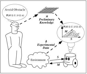
Figure 2 introduces the principle of this approach.
The fundamental notion is to place side by side the programmer’s conception of the task (the
prelimi-nary knowledge) and the experimental data to obtain probability distributions. These distributions can be used as programming resources.
Figure 2: The probabilistic approaches in robotics.
S
M
π
π
π
π
Preliminary
Knowledge
δδδ
δ
Experimental
Data
Avo id Ob stacle
P(M ⊗ S | δ⊗π)
S
M
Environment
Probalistic Methodology and Techniques for Artefact Conception and Development 5
The preliminary knowledge gives some hints to the robot about what it may expect to observe. The preliminary knowledge is not a fixed and rigid model purporting completeness. Rather, it is a gauge, with free parameters, waiting to be molded by the experimental data. Learning is the mean of setting these parameters. The pair made of a preliminary knowledge and set of experimental data is a description. The descriptions result from both the views of the programmer and the physical specificities of each robot and environment. Even the influence of the hidden variables is taken into account and quantified; the more important their effects, the more noisy the data, therefore the more uncertain the resulting probability dis-tributions will be.
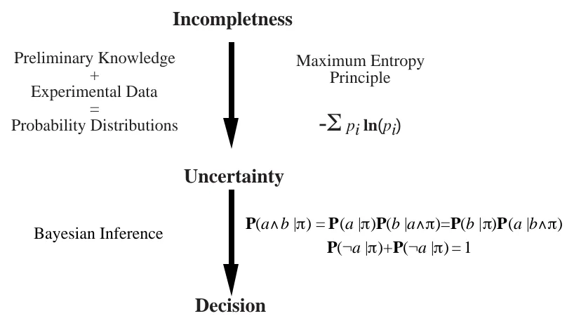
The probabilistic approaches to robotics usually need two steps as presented Figure 3.
The first step transforms the irreducible incompleteness into uncertainty. Starting from the
prelimi-nary knowledge and the experimental data, learning builds probability distributions. The prelimiprelimi-nary knowledge, even imperfect and incomplete, is relevant and provides interesting hints about the observed phenomenon. The more accurate and pertinent this preliminary knowledge is, the less uncertain and the more informational the learned distributions are.
The second step consists of reasoning with the probability distributions obtained by the first step. To do so, we only require the two basic rules of Bayesian inference. These two rules are to Bayesian infer-ence what the resolution principle is to logical reasoning (see Robinson, 1965; Robinson, 1979; Robinson & Sibert, 1983a; Robinson & Sibert, 1983b). These inferences may be as complex and subtle as those achieved with logical inference tools.
Development on these arguments may be found in 2 papers by Bessière (Bessière et al., 1998a & Bessière et al., 1998b).
Figure 3: Theoretical foundation.
Incompletness
Maximum Entropy
Principle
-
Σ
pi ln
(
pi
)
Preliminary Knowledge
+
Experimental Data
=
Probability Distributions
Uncertainty
Decision
P(a
∧
b |
π
) = P(a |
π
)P(b |a
∧π
)=P(b |
π
)P(a |b
∧π
)
Probalistic Methodology and Techniques for Artefact Conception and Development 7
2. A G
ENERICF
ORMALISM: T
HEB
AYESIANP
ROGRAMMINGIn this section, we introduce the concepts, postulates, definitions, notations and rules that are necessary to define a Bayesian program. The Bayesian Program (BP) formalism will then be used in the sequel of this paper to present, compare and comment on a number of probabilistic models.
It may appear very basic and obvious but one of the goal of this survey is to demonstrate that such simple rules and formalism are sufficient to present a unifying framework for most of the probabilistic approaches found in the literature.
2.1. Definition and notation
2.1.1. Proposition
The first concept we will use is the usual notion of logical proposition. Propositions will be denoted by lowercase names. Propositions may be composed to obtain new propositions using the usual logical oper-ators: denotes the conjunction of propositions and , their disjunction and the negation of proposition .
2.1.2. Variable
The notion of discrete variable is the second concept we require. Variables will be denoted by names starting by an uppercase letter.
By definition, a discrete variable is a set of logical propositions such that these propositions are mutually exclusive (for all with , is false) and exhaustive (at least one of the propositions is true). stands for «variable takes its value». denotes the cardinal of the set (the num-ber of propositions ).
The conjunction of two variables and , denoted , is defined as the set of proposi-tions . is a set of mutually exclusive and exhaustive logical propositions. As such, it is a new variable2. Of course, the conjunction of variables is also a variable and, as such, it may be renamed at any time and considered as a unique variable in the sequel.
2.1.3. Probability
To be able to deal with uncertainties, we will attach probabilities to propositions.
We consider that, to assign a probability to a proposition , it is necessary to have at least some
pre-liminary knowledge, summed up by a proposition . Consequently, the probability of a proposition is
always conditioned, at least, by . For each different , is an application assigning to each prop-osition a unique real value in the interval .
Of course, we will be interested in reasoning on the probabilities of the conjunctions, disjunctions and negations of propositions, denoted, respectively, by , and .
We will also be interested in the probability of proposition conditioned by both the preliminary knowledge and some other proposition . This will be denoted .
For simplicity and clarity, we will also use probabilistic formulas with variables appearing instead of propositions. By convention, each time a variable appears in a probabilistic formula , it should be understood as . For instance, given three variables , and ,
stands for:
[1]
2.2. Inference postulates and rules
This section presents the inference postulates and rules necessary to carry out probabilistic reasoning.
2.2.1. Conjunction and normalization postulates for propositions
Probabilistic reasoning needs only two basic rules:
1 - The conjunction rule, which gives the probability of a conjunction of propositions.
2. By contrast, the disjunction of two variables, defined as the set of propositions , is not a variable. These propositions are not mutually exclusive.
a∧b a b a∨b ¬a
a
X xi
i j, i≠ j xi∧yj
xi xi X ith X X
xi
X Y X∧Y X × Y
xi∧yj X∧Y
N
xi∨yj a
π a
π π P(.|π)
a P(a|π) [0 1, ]
a∧b|π
( )
P P(a∨b|π) P(¬a|π)
a
π b P(a|b∧π)
X Φ( )X
xi
∀ ∈X,Φ( )xi X Y Z P(X∧Y|Z∧π) = P(X|π)
xi
∀ ∈X,∀yj∈Y,∀zk∈Z xi∧yj|zk∧π
( )
[2]
2 - The normalization rule, which states that the sum of the probabilities of and is one.
[3] For the purpose of this paper, we take these two rules as postulates3.
As in logic, where the resolution principle (Robinson, 1965; Robinson, 1979) is sufficient to solve any inference problem, in discrete probabilities, these two rules ([2], [3]) are sufficient for any computa-tion. Indeed, we may derive all the other necessary inference rules from those two, especially the rules concerning variables.
2.2.2. Disjunction rule for propositions:
[4]
2.2.3. Conjunction, normalization and maginalization rules for variables
Conjunction (Bayes) rule
[5]
Normalization rule
[6]
Marginalization rule for variables
[7]
2.3. Bayesian Programs
Using these very simple postulates and rules it is possible to define a generic formalism to specify proba-bilistic models: Bayesian Programming (BP). This formalism will be used in the sequel of this paper to describe all the presented models.
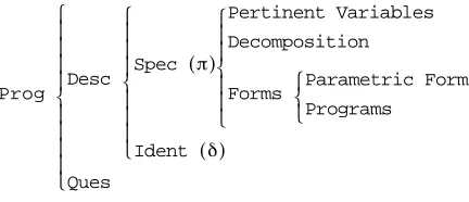
The elements of a Bayesian Program are presented Figure 4:
• A program is constructed from a description, which constitutes a knowledge base (declarative part), and a question, which restitutes via inference some of this knowledge (procedural part). • A description is constructed in 2 phases: a specification phase where the programmer expresses
its preliminary knowledge and an indentification (or learning) phase where the experimental data are taken into account.
• Preliminary knowledge is constructed from a set of pertinent variables, a decomposition of the joint distribution into a product of simpler terms, and a set of forms, one for each term. • Forms are either parametric forms or questions to other Bayesian programs.
3. Theoretical justifications of probabilistic inference and maximum entropy are numerous. The entropy concentration theorems (Jaynes, 1982; Robert, 1990) are among the more rigorous, Cox theorem (Cox, 1961) being the most well known, although it has been partially disputed recently by Halpern (Halpern, 1999a; Halpern, 1999b).
Figure 4: Structure of a bayesian program
a∧b|π
( )
P = P(a|π)×P(b|a∧π)
b|π
( )
P ×P(a|b∧π)
=
a ¬a
a|π
( )
P +P(¬a|π) = 1
a∨b|π
( )
P
a|π
( )
P +P(b|π)–P(a∧b|π)
( )
=
X∧Y|π
( )
P = P(X|π)×P(Y|X∧π)
Y|π
( )
P ×P(X|Y∧π)
=
X|π
( )
P
X
∑
= 1X∧Y|π
( )
P
X
∑
= P(Y|π)Prog Desc
Spec ( )π
Pertinent Variables
Decomposition
Forms Parametric Forms Programs
Ident ( )δ
2.3.1. Description
The purpose of a description is to specify an effective method to compute a joint distribution on a set of variables , given a set of experimental data and a preliminary knowledge . This joint distribution is denoted as: .
2.3.2. Preliminary Knowledge
To specify a preliminary knowledge the programmer must:
1 Define the set of relevant variables on which the joint distribution is defined. 2 Decompose the joint distribution:
Given a partition of into subsets, we define variables , each being the conjunction of the variables in each of these subsets.
The conjunction rules [5] leads to:
[8]
Conditional independence hypotheses then allow further simplifications. A conditional indepen-dence hypothesis for variable is defined by choosing some variables among the variables appearing in conjunction , calling the conjunction of these chosen variables and setting:
[9] We then obtain:
[10]
Such a simplification of the joint distribution as a product of simpler distributions is called a decomposition.
3 Define the forms:
Each distribution appearing in the product is then associated with either a para-metric form (i.e., a function ) or another Bayesian program. In general, is a vector of parameters that may depend on or or both. Learning takes place when some of these parameters are computed using the data set .
2.3.3. Question
Given a description (i.e., ), a question is obtained by partitioning into three sets : the searched variables, the known variables and the unknown variables. We define the variables , and as the conjunction of the variables belong-ing to these sets. We define a question as the distribution:
. [11] See section 4, “Bayesian Reasonning” on page 25, for all developments on how this question may be answered.
X1,X2,…,Xn
{ } δ π
X1∧X2∧…∧Xn|δ∧π
( )
P
X1,X2,…,Xn
{ }
X1,X2,…,Xn
{ } k k L1,…,Lk
X1∧X2∧…∧Xn|δ∧π
( )
P
L1|δ∧π
( )
P ×P(L2|L1∧ ∧δ π)×…×P(Lk|Lk–1∧…∧L2∧L1∧ ∧δ π)
=
Li Xj
Li–1∧…∧L2∧L1 Ri
Li|Li–1∧…∧L2∧L1∧ ∧δ π
( )
P = P(Li|Ri∧ ∧δ π)
X1∧X2∧…∧Xn|δ∧π
( )
P
L1|δ∧π
( )
P ×P(L2|R2∧ ∧δ π)×P(L3|R3∧ ∧δ π)×…×P(Lk|Rk∧ ∧δ π)
=
Li|Ri∧ ∧δ π
( )
P
fµ( )Li µ
Ri δ δ
X1∧X2∧…∧Xn|δ∧π
( )
P
X1,X2,... X, n
{ }
Searched Known Unknown
Searched|Known∧ ∧δ π
( )
3. B
AYESIANP
ROGRAMMINGANDM
ODELLINGThe goal of this section is to present the main probabilistic models currently used for artefact conception and development.
We will systematically use the Bayesian programming formalism to present these models. This is a good manner to be precise and concise and will simplify their comparison.
We will mainly concentrate on the definition of these models: discussions about inference and compu-tation will be postponed to section 4 and discussions about learning and identification will be postponed to section 5.
We chose to divide the different probabilistic models into 2 categories: the general purpose probabi-listic models and the problem oriented probabiprobabi-listic models.
In the first category, the modelling choices are made independently of any specific knowledge about the modeled phenomenon. Most of the time these choices are essentially made to keep with tractable inference. However, the technical simplifications of these models may be compatible with large classes of problems and consequetly may have numerous applications.
In the second category, on the contrary, the modelling choices and simplifications are decided accord-ing to some specific knowledge about the modeled phenomenon. These choices could eventually lead to very poor models from a computational point of view. However, most of the time, problem dependent knowledge like, for instance, conditional independence between variables, leads to very important and effective simplifications and computational improvements.
3.1. General Purpose Probabilistic Models
3.1.1. Graphical Models and Bayesian Networks
Bayesian Networks
Bayesian networks, first introduced by Judea Pearl (Pearl, 1988), have emerged as a primary method for dealing with probabilistic and uncertain information. They are the result of the marriage between the the-ory of probabilities and the thethe-ory of graphs.
They are defined by the following Bayesian program:
[12]
• The pertinent variables are not constrained and have no specific semantics.
• The decomposition, on the contrary, is specific: it is a product of distributions with one and only one variable conditioned by a conjunction of other variables called its "parents". An obvious bijection exists between joint probability distributions defined by such a decomposi-tion and directed acyclic graphs: nodes are associated to variables, and oriented edges are asso-ciated to conditional dependencies. Using graphs in probabilistic models leads to an efficient way to define hypotheses over a set of variables, an economic representation of a joint proba-bility distribution and, most importantly, an easy and efficient way to do probabilistic inference (see section 4.2.1).
• The parametric forms are not constrained but they are very often restricted to probability tables (this is, for instance, the case in the Bayesian networks commercial softwares such as Hugin4 or Netica5)
• Very efficient inference techniques have been developped to answer question ,
4. http://www.hugin.com/ 5. http://www.norsys.com/
Prog
Desc Spec
Pertinent Variables
X1,... X, N
Decomposition
X1∧...∧XN
( )
P P(Xi|Ri)
i=1
N
∏
=Forms
Any
Ident
Ques
Xi|Known
( )
P
Xi Ri
Xi|Known
( )
however some difficulties appear for more general questions (see section 4.2.1).
Readings on Bayesian nets and graphical models should start by the following introductory text-books: Probabilistic reasoning in intelligent systems : Networks of plausible inference (Pearl, 1988), Graphical
Models (Lauritzen, 1996), Learning in Graphical Models (Jordan, 1998) and Graphical Models for Machine Learning and Digital Communication (Frey, 1998).
Dynamical Bayesian Networks
To deal with time and to model stochastic processes, the framework of Bayesian Networks has been extended to Dynamic Bayesian Networks (DBN) (see Dean & Kanazawa, 1989). Given a graph represent-ing the structural knowledge at time t, supposrepresent-ing this structure to be time-invariant and time to be dis-crete, the resulting DBN is the repetition of the first structure from a start time to a final time. Each part at time t in the final graph is named a time slice.
They are defined by the following Bayesian program:
[13]
• is a conjunction of variables taken in the set . It means that depends only on its parents at time ( ) as in a regular BN and on some variables from the previous time slice ( ).
• defines a graph for a time slice and all time slices are identical when the time
index t is changing.
• A DBN as a whole, "unrolled" over time, may be considered as a regular BN. Consequently the usual inference techniques applicable to BN are still valid for such "unrolled" DBNs (see sec-tion 4.2.1).
The best introduction, survey and starting point on DBNs is the Ph.D. thesis of K. Murphy entitled
Dynamic Bayesian Networks: Representation, Inference and Learning (Murphy, 2002).
3.1.2. Recursive Bayesian Estimation, Hidden Markov Models, Kalman Filters and Particle Filters
Recursive Bayesian Estimation: Bayesian Filtering, Prediction and Smoothing
Recursive Bayesian Estimation is the generic denomination for a very largely applied class of numerous different probabilistic models of time series.
They are defined by the following Bayesian program:
Prog
Desc Spec
Pertinent Variables
X01,... X, 0N,... X, 1T,... X, TN
Decomposition
X10∧...∧XNT
( )
P P(X10∧...∧X0N) P(Xit|Rit)
i=1
N
∏
t=0
T
∏
× =Forms
Any
Ident
Ques
XiT|Known
( )
P
Rit {X1t,... X, it–1}∪{X1t–1,... X, tN–1}
Xit t {X1t,... X, it–1}
X1t–1,... X, Nt–1
{ }
Xit|Rit
( )
P
i=1
N
[14]
• Variables are a time series of "state" variables considered on a time horizon ranging from 0 to . Variables are a time series of "observation" variables on the same horizon.
• The decomposition is based:
° on , called the "system model" or "transition model", which formalized the tran-sition model from state at time i-1 to state at time i,
° on , called the "observation model", which expresses what can be observed at time i when the system is in state ,
° and on a prior over states at time 0.
• The question usually asked to these models is : what is the probability distribution for state at time t+k knowing the observations from instant 0 to t? The most com-mon case is Bayesian Filtering where , which means that you search for the present state knowing the past observations. However it is also possible to do "prediction" where one tries to extrapolate future state from passed observations, or to do "smoothing" where one tries to recover a past state from observations made either before or after that instant. How-ever, some more complicated questions may also be asked (see HMM further on).
Bayesian Filters have a very interesting recursive property which contributes largely to their inter-est. may be simply computed from with the following for-mula:
[15]
We give this derivation as an example of application of the rules presented in section 2.
Prog
Desc Spec
Pertinent Variables
S0,... S, N,O0,... O, N
Decomposition
S0∧...∧SN∧O0∧...∧ON
( )
P P(S0) P(O0|S0) [P(Si|Si–1)×P(Oi|Si)]
i=1
N
∏
× × = Forms S0 ( ) PSi|Si–1
( )
P
Oi|Si
( ) P Ident Ques
St+k|O0∧...∧Ot
( )
P
k=0
( )≡Filtering k>0
( )≡Prediction k<0
( )≡Smoothing
S0,... S, N
N O0,... O, N
Si|Si–1
( )
P
Oi|Si
( ) P Si S0 ( ) P
St+k|O0∧...∧Ot
( )
P
k = 0
k>0
( )
k<0
( )
k=0
( )
St|O0∧...∧Ot
( )
P P(St–1|O0∧...∧Ot–1)
St|O0∧...∧Ot
( )
P P(Ot|St) [P(St|St–1)×P(St–1|O0∧...∧Ot–1)]
St–1
[16]
Prediction and smoothing do not lead to such nice simplifications and suppose to make large sums that represent a huge computational burden.
Hidden Markov Models
The Hidden Markov Models (HMM) are a very popular specialization of Bayesian Filters. They are defined by the following Bayesian program:
[17]
• Variables are supposed to be discrete.
• The transition model and the observation models are both specified using probability matrices.
• The most popular question asked to HMMs is : what is the most probable series of states that leads to the present state knowing the past
observa-St|O0∧...∧Ot
( )
P
S0∧...∧SN∧O0∧...∧ON
( )
P
O0∧...∧Ot
( )
P
---Ot+1,... O, N
St+1,... S, N
∑
S0,... S, t–1
∑
=S0 ( )
P P(O0|S0) [P(Si|Si–1)×P(Oi|Si)]
i=1
N
∏
× ×O0∧...∧Ot
( )
P
---Ot+1,... O, N
St+1,... S, N
∑
S0,... S, t–1
∑
=S0 ( )
P P(O0|S0) [P(Si|Si–1)×P(Oi|Si)]
i=1
t
∏
× ×O0∧...∧Ot
( )
P
---. [P(Sj|Sj–1)×P(Oj|Sj)]
j=t+1
N
∏
Ot+1,... O, N
St+1,... S, N
∑
×S0,... S, t–1
∑
=S0 ( )
P P(O0|S0) [P(Si|Si–1)×P(Oi|Si)]
i=1
t
∏
× ×O0∧...∧Ot
( )
P
---S0,... S, t–1
∑
=1 Z
---×P(Ot|St) P(St|St–1)
S0 ( )
P P(O0|S0) [P(Si|Si–1)×P(Oi|Si)]
i=1
t–1
∏
× ×O0∧...∧Ot–1
( )
P
---S0,... S, t–2
∑
×St–1
∑
× =1 Z
---×P(Ot|St) [P(St|St–1)×P(St–1|O0∧...∧Ot–1)]
St–1
∑
× =Prog
Desc Spec
Pertinent Variables
S0,... S, t,O0,... O, t
Decomposition
S0∧...∧St∧O0∧...∧Ot
( )
P P(S0) P(O0|S0) [P(Si|Si–1)×P(Oi|Si)]
i=2
t
∏
× × = Forms S0 ( )P ≡Matrix
Si|Si–1
( )
P ≡Matrix
Oi|Si
( )
P ≡Matrix
Ident Ques
S1∧S2∧...∧St–1|St∧O0∧...∧Ot
( ) P
Si|Si–1
( )
P P(Oi|Si)
S1∧S2∧...∧St–1|St∧O0∧...∧Ot
( )
tions?
This particular question may be answered with a specific and very efficient algorithm called the "Vit-erbi algorithm" which will be presented in section 4.3.4.
A specific learning algorithm called the "Baum-Welch" algorithm has also been developped for HMMs (see section 5.2.3)
A nice start about HMM is Rabiner’s tutorial (Rabiner, 1989).
Kalman Filters
The very well known Kalman Filters (Kalman, 1960) are another specialization of Bayesian Filters. They are defined by the following Bayesian program:
[18]
• Variables are continuous.
• The transition model and the observation models are both specified using Gaussian laws with means that are linear functions of the conditioning variables.
Due to these hypotheses, and using the recursive formula [15], it is possible to analytically solve the inference problem to answer the usual question. This leads to an extremely efficient algorithm that explains the popularity of Kalman Filters and the number of their everyday applications.
When there is no obvious linear transition and observation models, it is still often possible, using a first order Taylor’s expansion, to consider that these models are locally linear. This generalization is com-monly called extended Kalman filters.
A nice tutorial by Welch and Bishop may be found on the Web (Welch & Bishop, 1997). For a more complete mathematical presentation one should refer to a report by Barker et al (Barker, Brown & Martin, 1994) but these are only 2 entries to a huge literature concerning the subject.
Particle Filters
The fashionable Particle Filters may also be seen as a specific implementation of Bayesian Filters. The distribution is approximated by a set of N particles having weights pro-portional to their probabilities. The recursive equation [15] is then used to inspire a dynamic process that produces an approximation of . The principle of this dynamical process is that the particles are first moved according to the transition model , then their weights are updated according to the observation model .
See Arulampalam’s tutorial for a start (Arulampalam et al., 2001).
3.1.3. Mixture Models
Mixture models try to approximate a distribution on a set of variables by adding up (mix-ing) a set of simple distributions.
The most popular mixture models are Gaussian mixtures where the component distributions are Gaus-sians. However, the component distributions may be of any nature as for instance logistic or Poisson dis-tributions. In the sequel, for simplicity, we will take the case of Gaussian mixtures.
Such a mixture is defined as follows:
Prog
Desc Spec
Pertinent Variables
S0,... S, t,O0,... O, t
Decomposition
S0∧...∧St∧O0∧...∧Ot
( )
P P(S0) P(O0|S0) [P(Si|Si–1)×P(Oi|Si)]
i=2
t
∏
× × = Forms S0 ( )P ≡G S( 0, ,µ σ)
Si|Si–1
( )
P ≡G S( i,A•Si–1,Q)
Oi|Si
( )
P ≡G O( i,H•Si,R)
Ident Ques
St|O0∧...∧Ot
( ) P
Si|Si–1
( )
P P(Oi|Si)
St|O0∧...∧Ot
( )
P
St–1|O0∧...∧Ot–1
( )
P
St|O0∧...∧Ot
( )
P
St|St–1
( )
P
Ot|St
( )
P
X1,... X, N
[19]
It should be noticed that this is not a Bayesian program. In particular, the decomposition does not
have the right form , as defined in equation [10].
It is, however, a very popular and convenient way to specify distributions . Espe-cially when the type of component distributions is chosen to insure nice and efficient analytical solutions to some of the inference problems.
Furthermore, it is possible to specify such mixtures as a correct Bayesian program by adding vari-ables to the previous definition:
[20]
• is a set of variables corresponding to the parameters of the component distributions. (i.e. the means and standard deviations in the Gaussian example).
• is a discrete variable taking values. is used as a selection variable. Knowing the value of , we suppose that the joint distribution is reduced to one of its component distribution:
[21]
• In these simple and common mixture models, , the mixing variable is suppose to be
indepen-Prog
Desc Spec
Pertinent Variables
X1,... X, N
Decomposition
X1∧...∧XN
( )
P [αi×Pi(X1∧...∧XN)]
i=1
M
∑
=Forms
Pi(X1∧...∧XN)≡G X( 1∧...∧XN,µi,σi)
Ident Ques
Searched|Known
( ) P
X1∧...∧XN
( )
P P(L1|δ∧π) P(Li|Ri∧ ∧δ π)
i=2
M
∏
× =X1∧...∧XN
( )
P
Pi(X1∧...∧XN)
Prog Desc
Spec
Pertinent Variables
X1,... X, N,Mu1,... Mu, M,Sigma1,... Sigma, M,H Decomposition
X1∧...∧XN∧Mu1∧...∧MuM∧Sigma1∧...∧SigmaM∧H
( )
P
Mu1∧...∧MuM∧Sigma1∧...∧SigmaM
( )
P ×P( )H
=
.×P(X1∧...∧XN|Mu1∧...∧MuM∧Sigma1∧...∧SigmaM∧H)
Forms
Mu1∧...∧MuM∧Sigma1∧...∧SigmaM
( )
P ≡Uniform
H ( )
P ≡Table
X1∧...∧XN|Mu1∧...∧MuM∧Sigma1∧...∧SigmaM∧[H=i]
( )
P
X1∧...∧XN|µi∧σi
( ) P = Ident H ( ) P
µ1,...,µM,σ1,...,σM
Ques
Searched|Known∧µ1∧...∧µM∧σ1∧...∧σM
( )
P
X1∧...∧XN∧Mu1∧...∧MuM∧Sigma1∧...∧SigmaM∧H
( )
P
H
∑
=H=i
[ ]
( )
P ×P(Searched|Known∧µi∧σi)
[ ]
i=1
M
∑
= Mu1,... Mu, M,Sigma1,... Sigma, M
{ }
M M
H M H
H
X1∧...∧XN|Mu1∧...∧MuM∧Sigma1∧...∧SigmaM∧[H=i]
( )
P
X1∧...∧XN|µi∧σi
( )
P
=
dent of the other variables. We will see in the sequel other mixing models where may depend on some of the other variables (see the combination model in section 3.2.7). It is also the case in expert mixture models as decribed by Jordan (see Jordan & Jacobs, 1994 or Meila & Jordan, 1996)
• Identification is there a crucial step where the values of and the parameters of the component distributions are searched in order to have the best possible fit between the observed data and the joint distribution. This is usally done using the EM algorithm or some of its variants (see section 5.2).
• The question asked to the joint distribution are of the form where and are conjunc-tions of some of the . The parameters of the compo-nent distributions are known but not the selection variable , which stays always hidden. Consequently, solving the question supposes to sum on the possible value of and we finally retrieve the usual mixture form:
[22]
A reference document on mixture models is McLachlan’s book entitled Finite Mixture Models
(McLachlan & Deep, 2000).
3.1.4. Maximum Entropy Approaches
Maximum entropy approaches play a very important role in physical applications. The late E.T. Jaynes, in his unfortunately unachieved book (Jaynes, 1995), gives a wonderful presentation of them as well as a fascinating apologia of the subjectivist epistemology of probabilities.
The Maximum entropy models may be described by the following Bayesian program:
[23]
• The variables are not constrained.
• The decomposition is made of a product of exponential distributions where each is called an observable function. An observable function may be any real function on the space defined by , such that its expectation may be computed:
. [24]
• The constraints on the problem are usually expressed by real values called level of
con-straint which impose that .
• The identification problem is then, kowing the level of constraint , to find the Lagrange
muti-pliers which maximize the entropy of the distribution .
The maximun entropy approach is a very general and powerful way to represent probabilistic models and to explain what is going on when one wants to identify the parameters of a distribution, choose its
H
H ( )
P
µ1,...,µM,σ1,...,σM
Searched|Known∧µ1∧...∧µM∧σ1∧...∧σM
( )
P Searched Known
X1,... X, N µ1∧...∧µM∧σ1∧...∧σM
H
H
Searched|Known∧µ1∧...∧µM∧σ1∧...∧σM
( )
P
H=i
[ ]
( )
P ×P(Searched|Known∧µi∧σi)
[ ]
i=1
M
∑
= Prog Desc Spec Pertinent VariablesX1,... X, N
Decomposition
X1∧...∧XN
( )
P
1 Z --- e
λi×fi(X1∧...∧XN)
[ ]
i=1
M
∑
– × = 1 Z--- e–[λi×fi(X1∧...∧XN)]
i=1
M
∏
× =Forms
f1,... f, M
Ident
λ1∧...∧λM Ques
Searched|Known
( ) P
X1,... X, N
e–[λi×fi(X1∧...∧XN)]
fi
X1∧...∧XN
fi(X1∧...∧XN)
〈 〉 [P(X1∧...∧XN)×fi(X1∧...∧XN)]
X1∧...
∑
∧XN=
M Fi
fi(X1∧...∧XN)
〈 〉 = Fi
Fi
form or even compare models. It, however, often leads to computations which are intractable.
A nice introduction is of course Jaynes’ book entitled Probability theory - The logic of science (Jaynes, 1995). References on the subject are the books, edited after the regular MaxEnt conferences, which cover both theory and applications (see Levine & Tribus, 1979; Erickson & Smith, 1988a; Erickson & Smith, 1988b; Kapur & Kesavan, 1992; Smith & Grandy, 1985; Mohammad-Djafari & Demoment, 1992 & Mohammad-Dja-fari, 2000).
3.2. Problem Oriented Probabilistic Models
3.2.1. Sensor Fusion
Sensor fusion is a very common and crucial problem for both living systems and artefacts. The problem is as follows: given a phenomenon and some sensors, how to get information on the phenomenon by putting together the information of the different sensors?
The most common and simple Bayesian modelling for sensor fusion is the following:
[25]
• is the variable used to describe the phenomenon, when are the variables encod-ing the readencod-ings of the sensors.
• The decomposition may seem peculiar as obviously
the readings of the different sensors are not independent from one another. The exact meaning of this equation is that the phenomenon is considered to be the main reason for the contin-gency of the readings. Consequently, it is stated that knowing , the readings are indepen-dent. is the cause of the readings and, knowing the cause, the consequences are independent. Indeed, this is a very strong hypothesis, far from being always satisfied. However it gives very often satisfactory results and has the main advantage of reducing considerably the complexity of the computation.
• The distributions are called "sensor models". Indeed, these distributions encode the way a given sensor responds to the observed phenomenon. When dealing with industrial sen-sors this is the kind of information directly provided by the device manufacturer. Hovever, these distributions may also very easily be identified by experimenting.
• The most common question asked to this fusion model is . It should be noticed that it is an inverse question. The capacity to easily answer such inverse questions is one of the main advantage of probabilistic modelling. This is not the only possible question, any question may be asked to this kind of model, and due to the decomposition most of them lead to tractable computations. For instance:
° makes the fusion of 2 single sensors. It sim-plifies nicely as the product of the 2 correponding sensor models.
° tries to measure the
coher-ence between the readings of 3 sensors and may be used to diagnose the failure of the kth
sen-sor.
Prog
Desc Spec
Pertinent Variables
Φ,S1,... S, N
Decomposition
Φ∧S1∧...∧SN
( )
P P( )Φ P(Si|Φ)
i=1
N
∏
× = Forms Any Ident QuesΦ|S1∧...∧SN
( )
P 1
Z
--- P( )Φ P(Si|Φ)
i=1
N
∏
× × =Searched|Known
( ) P
Φ {S1,... S, N}
Φ∧S1∧...∧SN
( )
P P( )Φ P(Si|Φ)
i=1
N
∏
× =Φ
Φ Si
Φ
Si|Φ
( )
P
Φ|S1∧...∧SN
( )
P
Φ|Si∧Sj
( )
P 1
Z
---×P( )Φ ×P(Si|Φ)×P(Sj|Φ) =
Sk|Φ∧Si∧Sj
( )
P 1
Z
3.2.2. Classification
The classification problem may be seen as the same one than the sensor fusion just described. Usually, the problem is called a classification problem when the possible value for is limited to a small number of classes and is called a sensor fusion problem when can be interpreted as a "measure".
A slightly more subtle definition of classification uses one more variable. In this model there are both the variable used to merge the information and to classify the situation. has much less values than and it is possible to specify which explicits for each class the possible values of . Answer-ing the classification question supposes to sum over the different values of .
The Bayesian program then obtained is as follows:
[26]
3.2.3. Pattern Recognition
Pattern Recognition is still the same problem than the 2 preceeding ones. However, it is called recognition because the emphasis is put on deciding a given value for rather than getting the distribution
.
Consequently, the pattern recognition community usually does not make a clear separation between the probabilistic inference part of the reasonning and the decision part using a utility function (see section 4.5). Both are considered as a single and integrated decision process.
A reference work on pattern recognition is still Duda’s book entitled Pattern Classification and Scene
Analysis (Duda & Hart, 1973).
3.2.4. Sequences Recognition
The problem is to recognize a sequence of states knowing a sequence of observations and, possibly, a final state.
In section 3.1.2 we presented the Hidden Markov Models (HMM) as a special case of Bayesian filters. These HMMs have been specially designed for sequence recognition, that is why the most common ques-tion asked to these models is (see equation [17]). That is also why a specialized inference algorithm has been conceived to answer this specific question (see section 4.3.4).
3.2.5. Markov Localization
Another possible variation of the HMM formalism is to add a control variable to the system. This extension is sometimes called input-output HMM (Bengio & Frasconi, 1995, Cacciatore & Nowlan, 1994, Ghahramani, 2001, Meila & Jordan, 1996), but, in the field of robotics, it has received more attention under the name of Markov Localization (Burgard et al., 1996, Thrun, Burgard & Fox, 1998). In this field, such an extension is natural, as the robot can observe its state by sensors, but can also influence its state via motor commands.
Starting from a HMM structure, the control variable is used to refine the transition model
of the HMM into , which is then called the action model. The rest of the HMM is unchanged. The Bayesian progam then obtained is as follows:
Φ Φ
Φ C C
Φ P(Φ|C) Φ
C|S1∧...∧SN
( )
P Φ
Prog
Desc Spec
Pertinent Variables
C,Φ,S1,... S, N
Decomposition
C∧Φ∧S1∧...∧SN
( )
P P( )C ×P(Φ|C) P(Si|Φ)
i=1
N
∏
× = Forms Any Ident QuesC|S1∧...∧SN
( )
P 1
Z
--- P( )C ×P(Φ|C) P(Si|Φ)
i=1
N
∏
× Φ∑
× = C C|S1∧...∧SN( )
P
S1∧S2∧...∧St–1|St∧O0∧...∧Ot
( )
P
A
Si|Si–1
( )
P
Si|Si–1∧Ai–1
( )
[27]
The resulting model is used to answer the question , which esti-mates the state of the robot, given past actions and observations: when this state represents the position of the robot in its environment, this amounts to localization.
A reference paper to Markov Localization and its use in robotics is Thrun’s survey entitled Probabilis-tic Algorithms in RoboProbabilis-tics (Thrun, 2000).
3.2.6. MDP & POMDP
Partially Observable Markov Decision Process
POMDPs are used to model a robot that has to plan and to execute a sequence of actions. A complete review of POMDPs and MDPs by Boutilier et al. (Boutilier, Dean & Hanks, 1999) is an interesting start-ing point.
Formally, POMDPs use the same probabilistic model than Markov Localization except that it is enriched by the definition of a reward (and/or cost) function.
This reward function models which states are good for the robot, and which actions are costly. In the most general notation, it therefore is a function that associates, for each couple state - action, a real valued number: .
The reward function also helps driving the planning process. Indeed, the aim of this process is to find an optimal plan in the sense that it maximizes a certain measure based on the reward function. This mea-sure is most frequently the expected discounted cumulative reward:
[28]
where is a discount factor (less than 1), is the reward obtained at time t, and is the mathemat-ical expectation. Given this measure, the goal of the planning process is to find a optimal mapping from probability distributions over states to actions (a policy). This planning process, which leads to intractable computation, is sometimes approximated using iterative algorithms called policy iteration or value itera-tion. These algorithms start with random policies, and improve them at each step until some numerical convergence criterion is met. Unfortunately, state-of-the-art implementations of these algorithms still can-not cope with state spaces of more than a hundred states (Pineau & Thrun, 2002).
An introduction to POMDPs is proposed by Kaelbling et al. (Kaelbling, Littman & Cassandra, 1998).
Markov Decision Process
Another class of approach for tackling the intractability of the planning problem in POMDPs is to suppose that the robot knows what state it is in. The state becomes observable, therefore the observation variable and model are not needed anymore: the resulting formalism is called a (Fully Observable) Markov Deci-sion Process (MDP), and is summed up by the following Bayesian program:
Prog
Desc Spec
Pertinent Variables
S0,... S, t,A0,... A, t–1,O0,... O, t
Decomposition
S0∧...∧St∧A0∧...∧At–1
( )
P
S0 ( )
P ×P(O0|S0) [P(Ai–1)×P(Si|Si–1∧Ai–1)×P(Oi|Si)]
i=1
t
∏
× = Forms Tables Ident QuesSt|A0∧...∧At–1∧O0∧...∧Ot
( )
P
1 Z
---×P(At–1)×P(Ot|St) [P(St|St–1∧At–1)×P(St–1|A0∧...∧At–2∧O0∧...∧Ot–1)]
St–1
∑
× = St|A0∧...∧At–1∧O0∧...∧Ot
( )
P
R
R S, i⊗Ai→ℜ
γt×Rt
t=0
∞
∑
〈 〉
[29]
• The variables are: a temporal sequence of states and a temporal sequence of actions.
• The decomposition makes a first order Markov assumption by specifying that state at time t depends on state at time t-1 and also on action taken at time t-1.
• is usually represented by a matrix and is called the "transition matrix" of the model.
MDPs can cope with planning in state-spaces bigger than POMDPs, but are still limited to some hun-dreds of states. Therefore, many recent research efforts are aimed toward hierarchical decomposition of the planning and modelling problems in MDPs, especially in the robotic field, where their full observabil-ity hypothesis makes their practical use difficult (Hauskrecht et al., 1998; Lane & Kaelbling, 2001; Pineau & Thrun, 2002 & Diard, 2003).
3.2.7. Bayesian Robot Programming
In his Ph.D. thesis, Olivier Lebeltel (see Lebeltel, 1999 and Lebeltel et al., 2003) proposes a methodology for programming robots taking into account incompleteness and uncertainty. This methodology is called BRP, for Bayesian Robot Programming. The capacities of this programming method have been demon-strated through a succession of increasingly complex experiments. Starting from the learning of sim-ple reactive behaviours, this work proposes probabilistic models of behaviour combination, sensor fusion, hierarchical behaviour composition, situation recognition and temporal sequencing. This series of experiments comprises the steps in the incremental development of a complex robotic program.
As an illustration of this approach, let us present a single example of these various problem dependent probabilistic models, called behaviour combination.
Combination
Suppose that we have defined or learned N different reactive behaviours, each one coded by a Bayesian program . It is possible to build a new Bayesian program as the combination of these N sim-pler ones. It is defined by:
Prog
Desc Spec
Pertinent Variables
S0,... S, t,A0,... A, t–1
Decomposition
S0∧...∧St∧A0∧...∧At–1
( )
P P(S0) [P(Ai–1)×P(Si|Si–1∧Ai–1)]
i=1
t
∏
× =Forms
Tables
Ident
Ques
A0∧...∧At–1|St∧S0
( )
P
S0,... S, t
{ } {A0,... A, t–1}
Si|Si–1∧Ai–1
( )
P
A∧Oi|πi
( )
[30]
• is a set of sensory variables, is a motor variable and is a selection vari-able.
• is a prior on the sensory variables, usually uniform.
• is a probabilistic model of which behaviour among the possibles is the most appropriate in a given sensory situation.
• is a selector which for each possible value of selects one of the behaviours.
• The question asked to this behaviour combination is : what is the distribu-tion on the motor variable knowing all the sensory inputs. As is unknown in this question, the answer is computed by summing on the different possible values of .
A first point of view on this combination is to consider that we have a probabilistic "if-then-else" or "case". Would the distribution be a collection of Diracs, we would have a regular "case" selecting one and only one value of (one behaviour) for each sensory situation. As may be more subtle by expressing relative probabilities for the different values of , we obtain instead a weighted sum of the different behaviours.
Another point of view on this behaviour combination is to consider that we define a special case of mixture models (see section 3.1.3) where the mixed models are the original reactive behaviours.
3.2.8. Bayesian CAD Modelling
Taking uncertainties into account in CAD systems is a major challenge for this software industry. Since the work of Taylor (Taylor, 1976), in which geometric uncertainties were taken into account in the manip-ulator planning process for the first time, numerous approaches have been proposed to model these uncer-tainties explicitly.
Gaussian models to represent geometric uncertainties and to approximate their propagation have been proposed in manipulator programming (Puget, 1989) as well as in assembly (Sanderson, 1997). Gaussian model-based methods have the advantage of requiring few computations. However, they are only applica-ble when a linearization of the model is possiapplica-ble, and are unaapplica-ble to take into account inequality con-straints.
Geometric constraint-based approaches (Taylor, 1976; Owen, 1993) using constraints solvers have been used in robotic task-level programming systems. Most of these methods do not represent uncertain-ties explicitly. They handle uncertainuncertain-ties using a least-square criterion when the solved constraints sys-tems are over-determined. In the cases where uncertainties are explicitly taken into account (as is the case in Taylor's system), they are described solely as inequality constraints on possible variations.
In his Ph.D. thesis, Kamel Mekhnacha (see Mekhnacha, 1999; Mekhnacha, Mazer & Bessière, 2000; Mekhnacha, Mazer & Bessière, 2001) proposes a Bayesian generic model of CAD modelling.
The main idea of Bayesian CAD modelling is to generalize the constraint-based approaches by taking into account the uncertainties on models. A constraint on a relative pose between two objects is repre-sented by a probability distribution on parameters of this pose instead of a simple equality or inequality. After the specification phase, in which a probabilistic kinematic graph, the joint distribution on the
Prog
Desc Spec
Pertinent Variables
O1,... O, N, ,A H Decomposition
O1∧...∧ON∧A∧H
( )
P
O1∧...∧ON
( )
P ×P(H|O1∧...∧ON)×P(A|O1∧...∧ON∧H) =
Forms
O1∧...∧ON
( )
P
H|O1∧...∧ON
( )
P
A|O1∧...∧ON∧[H=1]
( )
P ≡P(A|O1∧π1)
...
A|O1∧...∧ON∧[H=N]
( )
P ≡P(A|ON∧πN)
Ident Ques
A|O1∧...∧ON
( )
P 1
Z
--- [P(H|O1∧...∧ON)×P(A|O1∧...∧ON∧H)]
H
∑
× = O1,... O, N
{ } N A H
O1∧...∧ON
( )
P
H|O1∧...∧ON
( )
P N
A|O1∧...∧ON∧H
( )
P H N
A|O1∧...∧ON
( )
P
H
H
H|O1∧...∧ON
( )
P
H H|O1∧...∧ON
( )
P
H