3213
Speed Estimation In DC Motor Using Raspberry
Pi Processor
Dr. R.subasri, A.AarthyAbstract—The Kalman filter is a state estimation algorithm applied to the system or to the processes in industries that involves noisy measurement from sensors. The estimation is based on prediction from past outputs and the current measurement along with process and measurement noise that are present with in the process. The Kalman gain is found out with the objective of minimizing the cost function (apriori covariance) approximately to zero. The sensor noise in the proximity sensor (for speed measurement) along with the process noise in DC motor is filtered through Kalman filter. The performance of Kalman filter is verified in simulation using windows OS and its real time implementation was done by dumping the Kalman filter algorithm coded in Python in to the Raspberry Pi. From the results, it is observed that the noise covariance is gradually reduced which indicates that the Kalman filter produces the noise free speed estimation of DC motor.
Index Terms—Kalman filter (KF), Raspberry Pi (RPi), MATLAB, Noise covariance, Speed estimation, proximity sensor, DC motor, —————————— ——————————
1
INTRODUCTION
The Kalman Filter is a widely used technique in filtering and estimation problems in many branches of the sciences. Its efficiency and easy implementation made it a well-known tool capable of achieving outstanding results in applications where the data is corrupted by additive noises. Control engineering concerns the efficient automated control of diverse kinds of industrial and other processes. An example would be regulating the flow of gas within a gas network, while minimizing the amount of energy expended on driving the gas through the pipes. This is achieved by monitoring a limited number of flow and pressure measurements from the network, and using this information to guide the control of the compressors and valves. This is known as feedback control. Some states are measurable easily by the sensor but some could not be directly measurable. Knowing the full state of an industrial plant is important for both safety and efficient control. However, only a limited amount of measurement data may be available. This may be due to the expense or difficulty of incorporating sensors into a plant. With limited measurement data, various techniques may be used that will produce an estimate of the entire state of the system. State estimators provide a cheap alternative to add new sensors or upgrading existing ones. These unmeasurable sensors can be made measurable by application of state estimation. The function of state estimator is to construct the current state vector from the time history of past sensor outputs. Python is an interpreted general-purpose, object oriented high-level programming language. It has vast applications over various fields and used for all engineering and non-engineering applications Python is supported by a vast collection of standard and external software libraries.Since last decade Python becomes one of the most popular programming languages for interfacing applications.
_______________________
Dr. R Subasri is professor at Electronics and Instrumentation Engineering department , Kongu Engineering College, Perundurai,
Erode, Tamil Nadu, India. PH-9965527506.
E-mail:[email protected]
A. Arrthy was the PG scholar at Electronics and Instrumentation Engineering department , Kongu Engineering College, Perundurai, Erode, Tamil Nadu, India. PH-8012357409. E-mail: [email protected]
The Kalman filter algorithm written in Python code is embedded in to the Raspberry Pi processor under Linux operating system and made to run to produce the noise free speed estimation in real time.
2
STATE
ESTIMATION
Full-state feedback is usually not practical because it is not possible (in general) to measure all the states. In practice, only certain states are measured and provided as system outputs. The states that are unmeasurable lead to the concept of state estimation. The state estimation of the deterministic system (noiseless) is called Luenberger Observer. The state estimation of stochastic system (noisy) system introduces an algorithm called Kalman filter. Kalman Filter is a commonly used method to estimate the values of state variables of a dynamic system that is excited by stochastic (random) disturbances and stochastic (random) measurement noise. The motivation problem for the Kalman Filter is to estimate the states of a linear system corrupted by noise. For instance, such noise can be the result of imperfections from the dynamical process of the system (called process noise) and from the measurement equipment used to read its output (called measurement noise). The noise is modeled as a white noise with zero mean in cases from which the filter is designed to be unbiased. Furthermore, in many engineering applications, the noise is assumed to be Gaussian, i.e., it is completely described by its mean and covariance. However, it has been proved that the filter also works with different assumptions for noise although the procedure for obtaining its equations became much more complex and lengthier. The application of Kalman filter includes Determination of planet orbit parameters from limited earth observations, Tracking targets – eg., aircraft, missiles using RADAR, Robotic tracking, At space research centers, DRDO, to determine position and velocity of satellites, Image processing, Traffic management systems, Interfaced along with GPS, Flux in Induction motor and Level estimation in process control systems.
2.1 Initial Assumptions
Some of the assumptions that are to be made before state estimation in Kalman filer are:
3214 cov[w(t),v(t)]=0
The process noise covariance (Q) and the measurement noise covariance (R) matrix are generally designed to be Gaussian or else the process noise covariance is chosen according to the uncertainity in the process.
cov[w(t),w(t)]=Q(t) cov[v(t),v(t)]=R(t)
The value of error covariance is calculated by using a set of past measurements. This initial value of covariance ) is called apriori covariance. This value has to be computed during the offline condition initially.
P(x0) =cov [x0(t), x0(t)]
2.2 Selection of Process Noise covariance
Designing of process noise (Q) is the most difficult and challenging one apart from Kalman filter implementation procedure. Process noise most probably could not obtain accurately since process involved mostly is of non-linear in nature. So randomly it may assume to be of Gaussian white noise of zero mean. For example, consider the refrigerator in which state is a temperature and is measured by using temperature sensor. The temperature at nth time was examined to be 5 degree Celsius and then after at (n+1)th it is 7 degree Celsius . It could not be concluded that the process noise is of 2 degree Celsius, because, 1.the refrigerator contains the condenser that ON and OFF over a threshold range and also 2. It depends on the climatic condition of atmosphere and there may poor insulation of door, and 3.one may interrupt the door (opening and closing) during the condensation. These are the various aspects that make the process noise undesirable. But due to this we could not make the ‗Q‘ to be ‗very small‘ because the Kalman filter will not behave well and if considering ‗Q‘ to be ‗large‘ the measurement will deviate large from estimated, resulting in poor design of filter. So randomly it is assumed to be Gaussian for these types of cases. Even by implementing this Kalman filter will not eliminate the noise. So the primary purpose is to minimize the effect of measurement noise and not the process noise. The state does not fluctuate over time without the influence of process noise. It is in the sense that Kalman filter will incorporate the process noise in predicting the actual state better, rather than eliminating the process noise. Thus process noise is used in estimation of actual value of measurement thus making it a error free sensor output. As an another case, consider the flying cannon‘s ball in which the process noise is the wind direction and velocity, floor‘s irregularity, etc., which should be considered for evaluating of process noise. Another good example is the state estimation in power system cables where the process noise is considered as harmonics and the Q is computed accordingly. Similarly for tracking of car the process noises are influence of wind flow, dig on road, speed breakers etc. So design of noise covariance is an important task in Kalman filter design. Even though as there are more cases trying to design process noise to its utmost, it is only by assumptions and not accurate and hence results in unfair precision of
process noise design. But the measurement noise covariance (R) could be found appreciably and easily by taking the continuous set of measurement values and calculating the mean and covariance accordingly. The design of process and measurement noise covariance matrices for a white noise is referred in [1].
2.3 State estimation Implementation procedure
The Kalman filter used here is Discrete Kalman filter. The first step is the creation of model. The state space model of the system is:
System dynamics :𝑋̇ = 𝐴𝑋 + 𝐵𝑈 + 𝐺𝑊 Measured output : Y=CX+V
where , W:process noise vector
V:sensor noise vector. Both V and W are uncorrelated white noise with auto-covariance as Q and R respectively .
Initialize the state x(0).Initialize the covariance of the x(0), which is computed as,
𝑃 = 𝐸[𝑋 0). 𝑋 0) ]
This covariance is the apriori covariance that is used to find the Kalman gain, Kek. The kalman gain is computed such that the covariance must be minimum with the proper selection of gain,
i.e., To minimize ,𝐽 = 𝑇𝑟 𝑘) ) Such that the gain obtained is.,
1
]
[
T k
k k k T k k
ek P C C P C R
K
From the measurement and estimated gain ,the estimated state at the present instant is computed as.,
[ ]
k ek k k k
k X K Y C X
X
The covariance for the next iteration is updated using the present measurement. This covariance is called as Posteriori Covariance,which is computed by using apriori covariance matrix and noise as.,
T ek k ek T k ek k
k ek
k I K C P I K C K R K
P ( ) ( )
The propagation follows the prediction of state for the next iteration of measurement and prediction of apriori covariance matrix from previously updated posteriori matrix.
The prediction of state is given as ., Xˆk AkXˆkBkUk
while the predicted value for covariance is obtained using Lyapunov Equation .,
𝑃̇ 𝑡) = 𝐴𝑃 + 𝑃𝐴 + 𝐺𝑄𝐺
The above step gets repeated for every new value of measurement and estimated state is thus obtained, until the Apriori covariance value converges to its least minimum value
3
NEED
OF
PYTHON
AND
RASPBERRY
PI
IN
REAL
TIME
IMPLEMENTATION
3215 RAM so it can now run bigger and more powerful
applications. The advantage of choosing Raspberry Pi is that it can run both as processor as well as controller. The Raspberry pi B+ model is used here for implementation. The architecture of Raspberry pi B+ is shown in figure
This version of B+ processor provides additional features such as 40 pins in GPIO (General Purpose Input Output), which is necessary for sensor connection, micro storage Device (SD) for installation of operating system and storage, High Definition Multi-Media Interface for external audio and video support., 4 USB ports etc .The Raspberry pi board could be given supply through the data cable. The maximum supply to Raspberry Pi is 5v DC. There is also a supply of 3.3v DC in GPIO port. Raspberry Pi can be accessible in monitor through Ethernet port in board and can made to run in either static or in dynamic mode of configuration. The python is installed in to the Linux operating system of Raspberry Pi by using the below command.
― sudo apt-get install python ‖
The version here refers to python 2.7. The packages that is necessary to be used in python for Kalman filter implementation is numpy, matplotlib, time and Rpi.GPIO. Numpy is a package for efficient handling of large arrays and matrices of numerical data. Matplotlib is a package for creating 2D plots and graphs. These two package are necessarily to be used here for Kalman algorithm. The latter two packages are required to use the board implementation in python. The package RPi. Gpio is used for accessing GPIO pins in python where as the package time is installed to access and control the time specification of board. The required packages are downloaded at online by using the board at dynamic state. The command used is ― sudo apt-get install packagename ‖.
4
REAL
TIME
IMPLEMENTATION
OF
KALMAN
FILTER
IN
DC
MOTOR
The objective is to estimate the states of the motor from noisy measurement at online condition, using the process and measurement noise covariances obtained during offline condition. The real time speed values are measured through Proximity sensor which gets processed through Kalman filter algorithm (coded in Python) embedded in Raspberry Pi (act both as processor and controller) and the estimated value of speed is obtained.
4.1 Model Creation of system
The DC motor provides the mechanical output that is measured in terms of speed by using various sensors. The sensor used here is the Inductive proximity sensor. The motor itself has some noise due to magnetic flux linkage, environmental loss, heat loss etc., which may give inaccurate measurement data, these are referred as process noise. The sensor itself has some inaccuracy in measurement, this may due to poor calibration, poor interface with sensor etc., this is referred as measurement noise by the sensor. The Process noise covariance(Q) and measurement noise covariance(R) value must be chosen such that it eliminates the noises that present in the system. The values are chosen here based on white space model [1]
as R=0.01 and .
The state of the system represents the angular velocity( =
𝜔) and angular acceleration( = 𝜔̇) of the motor.
2 1 x x x
The state space form is given as., ̇ = 𝐴 + 𝐵𝑢
[ ̇ ̇ ] = [
0
0 ] [ ] + [ 0 𝑘 ] 𝑢 where., J R k k a t 1 J R k k p a b t 1
kb = back emf constant .
Ra = armature resistance(in ohm). La =armature inductance(henry). kt=Torque constant.
θ(s)= Angular position (in rad). U(s)= Input voltage(in volt).
The constants and are calculated as 4.10 and 5.55. Discretizing state space form.,
5741 . 0 0 0767 . 0 1 0 ] 1 [ 1 1 1 1 1 Tp Tp AT e e p e F
0.31460172 . 0 ] 1 [ 1 [ . 1 1 1 1 1 1 1 0 hp hp T A e p k p e h p k d b e g
1 0
c
The output equation is represented as, Y=CX
2 1 0 1 x xThe initial value of state is taken as 01 . 0 01 . 0 0 X
The initial value of Apriori covariance is chosen such that it represents auto correlation of the initial state of the system.
003 . 0 0 0 43 . 39
P . The off-diagonal elements are zero,
since noises are uncorrelated their cross correlation is equal to
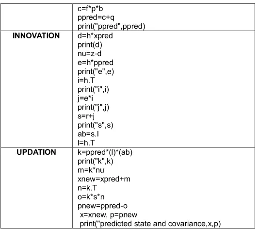
zero. The three steps of Kalman filter with its corresponding Python code is depicted in Table. I
4.2 Kalman Algorithm Coding for implementation
TABLE I.
KALMAN IMPLEMENTATION STEPS STAGES CODING USING PYTHON
PREDICTION xpred=f*x
3216 c=f*p*b
ppred=c+q print("ppred",ppred) INNOVATION d=h*xpred
print(d) nu=z-d e=h*ppred
print("e",e) i=h.T
print("i",i) j=e*i
print("j",j) s=r+j
print("s",s) ab=s.I
l=h.T
UPDATION k=ppred*(l)*(ab) print("k",k) m=k*nu xnew=xpred+m n=k.T
o=k*s*n pnew=ppred-o x=xnew, p=pnew
print("predicted state and covariance,x,p)
The coding is checked for its accuracy by giving the measurements manually.
4.3 Interfacing of Sensor with Raspberry Pi
The Raspberry Pi posses the capability of handling real time data through GPIO from proximity sensor. The Linux operating system is installed in to SD of Raspberry pi using Open CV. The new text editor is created where the coding is done to get the GPIO input and pass it to Kalman filter algorithm to obtain the estimated speed. By using the following command the text editor is created, where ―measuregpio‖ refers to the filename where the coding is placed. After that sensor is made to interface with the GPIO of Raspberry Pi and obtain the value of speed directly from sensor and pass it for Kalman implementation. The supply terminal to the sensor is given to 5v DC terminal of Raspberry Pi(1 in board), the ground sensor connection to ground terminal of board(3 in board), the output terminal to one of the input-output terminal of GPIO pins(11 in board or 18 in BCM). This output pin‘s voltage gives the required sensor pulse that is used to calculate the speed of motor. Every rotation of motor gives one pulse of voltage. Thus the number of pulse generated per 60 second at the output pin of sensor gives the rpm of motor. The program is made in such a way that the pulse count for one minute is measured through the input to GPIO. This measured rpm of sensor is noisy, thus passed to the Kalman algorithm to obtain the estimated speed.
4.4 Overview of Experimental setup
The Proximity sensor from which the speed has to be measured is interfaced with the rotor of DC motor, which gives pulse on every rotation of motor. The sensor voltage range is of (0-36) V which is biased through RPS of 6V. The proximity sensor produces output voltage when it comes in contact with the metallic substances (Here, metallic strip attached to rotor). Hence the sensor produces 36V on each rotation of motor, which could not be interfaced directly with the RPi (in GPIO). Thus the voltage divider circuit is used to reduce the voltage lesser than 5V. Here the magnitude of voltage does not play any role since only the frequency determines the speed of rotor. The voltage pulse is obtained
on every rotation of rotor at GPIO terminal. The coding to detect the number rising and falling of pulses per minute is saved within the processor is enabled by the user.
This gives the frequency of pulse and hence the RPM of motor. The specifications of DC motor used in real time implementation in the micro controller were tabulated as in table-2 and the experimental setup is shown in Figure 2.
Figure 2. Block Diagram of Experimental Setup
TABLE 2. DC Motor Specifications
PARAMETER RANGE
Speed range 0 to 1200 rpm
Signal conditioning IC conditioning circuit DC Power Supply DC 12V /0.1A for IC circuit System output Digital meter to monitor the
speed
Input supply AC 220V 10% ,50Hz,Single Phase
Sensor – DC motor with sensor arrangement mounted on an insulated base plate
Inductive Proximity Sensor
5
RESULTS
AND
DISCUSSION
When the motor is in running condition, the python code for Kalman algorithm is executed. For every measured value from the speed sensor, the processor gives the filtered noise free speed value and the related noise covariance. The coding requires the ‗import‘ of numpy, Rpi and time packages for the execution. The ‗Numpy‘ package is to use matrices in Kalman filtering algorithm. The ‗Rpi‘ package is to include hardware functionalities of Raspberry Pi in to the Python. The command execution hierarchy is given in table-3.The ‗time‘ package is to set the time duration to count the pulses for every 60 seconds. The measured and estimated speed values are compared in Fig 3. From the results, it is observed that the noise covariance is gradually reduced which indicates that the Kalman filter produces the noise free speed estimation. Since the chosen covariance value is very small, the estimated value of speed is closer to the speed measurement obtained from sensor. As there is only one sensor involved in this implementation, two or more sensors should be applied to acquire precise value of estimation, thus leading to the concept called sensor fusion.
TABLE 3. Command Execution Hierarchy COMMAND EXECUTION REMARKS
pi@raspberrypi ~ $ su Switch user
Password : Entering password for switch user root@raspberrypi ~ $ cd
name
3217 root@raspberrypi
:/home/source folder# nano filename.py
Opens the file in which the program has been saved. Type the program and save it by giving “ ctrl+x ”
root@raspberrypi
:/home/source folder# python filename.py
Runs the program and displays the measurement value and Estimated value. Thus estimated state depends on covariance chosen, and covariance depends on noise present in parameters of kalman filter.process. Therefore it is the noise that determines the parameters of kalman filter. The Fig 4 shows variation of covariance at each iteration.
Fig., 3 Measured speed Vs Estimated speed
Fig., 4 Variation of Covariance at every iteration
The figure 4 gives the plot of the trace of a priori covariance matrix obtained at each iteration of measurement. This shows that the covariance decreases for every measurement giving out an error free speed value.
6
CONCLUSION
Kalman filter is a powerful tool for estimating the state of any linear or non linear system by eliminating the sensor and process noise. In this paper, the DC motor is considered and its speed estimation is done through the Kalman algorithm. The sensor noise in the proximity sensor along with the process noise in DC motor is filtered through Kalman filter. The performance of Kalman filter is verified in real time by dumping the Kalman filter algorithm coded in Python in to the Raspberry Pi. From the results, it is observed that the noise covariance is gradually reduced which indicates that the Kalman filter produces the noise free speed estimation. This proves the reliability of kalman filter. The estimated noise free
speed from the Kalman filter can be given to a feedback controller to control the speed of the DC motor. Since the Raspberry Pi acts as both processor and controller, the same processor can also be used for controlling the speed by connecting the L298n driver which controls the voltage source to motor. The sensor fusion is invoked that uses multiple sensor measurement to acquire the precise estimation of speed.The Kalman filter algorithm coded in Python which is embedded in RPI processor can also be used to estimate the process parameters in any process control applications and also for image and signal processing applications such as ECG, EEG, EOG analysis.
REFERENCES
[1] Roger R.Labbe(2015) , ‗Kalman and Bayesian filters in Python ‗,creative common attributions 4.0 international licence.
[2] Saneej B. Chitralekha, Sirish L. Shah, J. Prakash(2010) ,‘Detection and quantification of valve stiction by the method of unknown input estimation ‗ ,Journal of Process Control, Volume 20, Issue 2,, Pages 206-216. [3] Roger M. du Plessis (1957), ‗Poor man‘s explanation of
kalman filtering‗,North American Rockwell Electronics group.
[4] Mohamed laaraiedh (2010),‘ Implementation of Kalman Filter with Python Language ‗, IETR Labs, University of Rennes.
[5] Jerker Nordh (2013), ‘A Python Framework for Particle Based Estimation Methods‘ Journal of Statistical Software, Lund University.
[6] Jie Meng (2014),‗Research on Optimal Control for the Vehicle Suspension Based on the Simulated Annealing Algorithm‗,Hindawi Publishing Corporation ,Journal of Applied Mathematics ,Volume 2014, Article ID 420719. [7] Navid Razmjooy, Mehdi Ramezani2, Esmaeil Nazari
(2015),‘Using LQG/LTR optimal control method for car suspension system‘,Scro Research Annual Report, Volume. 3, pages. 1-8.
[8] Diogo Marques, Luís Perdigoto et all., ―DC motors control using active observers‖, 4th Portuguese conference on Automatic Control ISBN 972-98603-0-0, 2000.
[9] M. Ruderman, J. Krettek et all., ―Optimal State Space Control of DC Motor‖ ., The International Federation of Automatic Control, 2008.
[10]Silverio Bolognani , ―Extended Kalman Filter Tuning in Sensor less PMSM Drives‖ , ,ieee transactions on industry applications,,Dec 2003 .
[11]Sheikh Ferdoush, Xinrong Li, ―Wireless Sensor Network System Design using Raspberry Pi and Arduino for Environmental Monitoring Applications‖ ,the 9th International Conference on Future Networks and Communications , Procedia Computer Science 34 ( 2014 ) 103 – 110 .,2014.
[12]Neethu John, Surya R, ―A Low Cost Implementation of Multi-label Classification Algorithm using Mathematica on Raspberry Pi‖ ,International Conference on Information and Communication Technologies, Procedia Computer Science 46 ( 2015) 306 – 313 .,2014.
3218 [14]Jaime Gomez-Gil Ruben Ruiz Gonzalez (2013), ‗A
Kalman Filter Implementation for Precision Improvement in Low-Cost GPS Positioning of Tractors‗, sensors Article,ISSN 1424-8220.
[15]Neethu John, Surya R, ―A Low Cost Implementation of Multi-label Classification Algorithm using Mathematica on Raspberry Pi‖ ,International Conference on Information and Communication Technologies, Procedia Computer Science 46 ( 2015 ) 306 – 313 .,2014.