The Influence of Inconsistent Data on Cost- Sensitive Classification Using Prism Algorithms: An Empirical Study

The Influence of Inconsistent Data on

Cost-Sensitive Classification Using Prism Algorithms:

An Empirical Study

College of Information System and Management, National University of Defense Technology, Changsha, China Email: {haozhiyongphd, liyao6522, nudtwyj}@gmail.com

Abstract—Cost-sensitive classification is one of the hottest research topics in data mining and machine learning. It is prevalent in many applications, such as Automatic Target Recognition (ATR), medical diagnosis, etc. However, the data in practice may be inconsistent due to dimensional reduction operation or other pre-processing, yet it is not clear how the inconsistent data affects cost-sensitive learning. This paper presents an empirical comparative study using four Prism rule-generating algorithms with J-measure pruning, two of which are proposed in this paper. The most important result of our study is that inconsistent data dose often affects the performance of cost-sensitive Prism classifiers, and in the inconsistent data setting, merely a single Prism classifier’s robustness cannot completely satisfy the requirements of cost-sensitive systems.

Index Terms—cost-sensitive, classification, Prism algorithm, inconsistent

I. INTRODUCTION

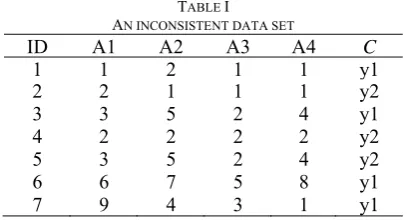
In classification rule inductive learning, different misclassification often involve different costs, that is when unseen instances are misclassified, they may incur different cost of errors depending on whether they are false negatives (classifying a positive instance as negative) or false positive (classifying a negative instance as positive) [1]. This is prevalent in many applications, such as Automatic Target Recognition (ATR), event detection, medical diagnosis, etc. For instance, in oil-slick detection, the cost of failing to detect an environment-threatening real slick is far greater than the cost of a false alarm. Generally, in inductive concept learning tasks (i.e. binary inductive learning tasks), given an example space and a target concept, the task is to find a hypothesis such that every example is satisfied[2].However, in real-world applications, data sets may often be inconsistent[3] due to dimensional reduction operation or other data pre-processing. The inconsistent data sets contain conflict examples, such examples are characterized by identical values for all attributes yet these examples belong to different classes. An example of the inconsistent dataset is presented in Table I, where examples 3 and 5 have the same attribute values, but class labels are different. In this case, there is no learnt hypothesis that could classify the conflict examples perfectly.

Various cost-sensitive induction of decision trees have been developed to deal with different costs of classification errors, such as[4, 5]. Decision tree inductive learning is based on the ‘divide and conquer’ rule induction approach, which induces classification rules in the intermediate form of decision tree[6]. A more general approach to inducing classification rules is ‘separate and conquer’ approach, which is also called the covering algorithms[7]. The covering algorithm induces a set of IF…THEN rules that do not necessary fit into a decision tree representation, and will not suffer from the ‘replicated subtree problem’. This alternative approach to decision tree has its several modern representatives, such as the Prism family of algorithms[8]. On the other hand, learning form inconsistent data is also a non-trivial problem, because the completeness and consistency criteria in inductive learning can no longer be fulfilled[9].

However, previous research mainly focus on pure cost-sensitive learning or pure learning from consistent data, largely ignoring the fact that inconsistent data and unequal misclassification costs may occur simultaneously. Although it has been observed that inconsistent data has certain influence on cost-sensitive induction of decision tree classifiers[10], to the best of our knowledge, there is no thorough empirical study for the influence of inconsistent data on cost-sensitive learning with covering algorithms, such as Prism family of algorithm.

settings, we have to pay more attention to ensemble of different learning algorithms.

TABLE I AN INCONSISTENT DATA SET

ID A1 A2 A3 A4 C

1 1 2 1 1 y1 2 2 1 1 1 y2 3 3 5 2 4 y1 4 2 2 2 2 y2 5 3 5 2 4 y2 6 6 7 5 8 y1 7 9 4 3 1 y1

This paper is structured as follows: In the next section, we give a brief description of the basic Prism framework. In Section III, we discuss J-measure pruning and four different rule-generating strategies used in our empirical study. Section IV gives some commonly used performance metrics in the cost-sensitive classification problems and the experiments study is presented in Section V. Finally, we discuss the main conclusions from this study and point some directions for future research.

II. THE BASIC PRISM ALGORITHM FRAMEWORK As mentioned in the introduction, the Prism family of algorithms has shown to produce similar classification accuracy compared with decision trees, and even outperforms decision trees when the training data is noisy[12]. The original Prism algorithm was introduced by Cendrowska[13], whose aim is to induce modular classification rules directly from the training set. The basic algorithm generates the rules concluding each of the possible classes in turn, and each rule is generated term by term, which is in the form of ‘attribute-value’ pair. The ‘attribute-value’ term added at each step is chosen to maximize the separation between the classes.

Figure 1. Pseudo code for the basic for Prism algorithm

The basic form of Prism algorithm is shown in Figure 1, where the training set is restored to its original state each time around. The step 1 to 4 iterates over the classes and generating rules for each class in turn. While creating

rules for that class, remove the examples from the set until there is none of that class left. Whenever a rule is created, it starts with an empty form, which covers all the examples, and then it is restricted by adding tests until it covers only examples of the desired class. At each stage, the most promising attribute-value test will be chosen, that is the one that maximizes the accuracy of the rule. In addition, the ties should be broken by selecting the test with greatest coverage.

III. STRATEGIES FOR GENERATING RULES IN PRISM WITH J-MEASURE PRUNING

This section is used to introduce the particular rule-generating strategies for Prism algorithm considered in this paper. We pay attention to J-measure pruning, an efficient facility for the information theoretic pruning of modular classification rules, which aims to prevent classifiers from overfitting on the training sets. We will first describe the basic principle of J-measure pruning in subsection A. As well as the basic version of Prism, two other rule-generating strategies are described, which are called TC and TCS[11]. These two strategies select the class with largest or smallest examples in the training set as the target class for the starting of basic Prism algorithm, and the rules generated by these two strategies must be fired in order. Two other rule-generating strategies have been proposed in this paper apart from the previous variations of Prism, which is described in subsection B.

A. J-measure Pruning

Just like any classification rule induction algorithm, pruning methods can also be used to prevent Prism algorithm from overfitting on the training set. Generally, pruning methods are divided into categories, pre-pruning and post-pruning. Pre-pruning is applied during the classification rule induction process, while post-pruning is applied after it has been induced. J-pruning[11] is pre-pruning method, which can be applied both to decision tree algorithms and Prism algorithms, and has shown good results on both of them. In addition, it is also found that J-pruning reduces the number of rules and rules terms induced considerably in the parallel version of Prism[14]. J-Pruning is based on J-measure[15]，_a quality measure for the information content of a rule.

According to Smyth and Goodman[15], as a means of quantifying the information content of a rule, J-measure is based on information theory. Given a rule of the form IFA =aTHENC=c, the information content of the rule, measured in bits of information is called J-measure, which is denoted by ( ;J C A=a):

J C A( ; =a)=p a j C A( ) ( ;i =a) (1) where ( )p a is the probability that the antecedent of the rule will occur, and ( ;j C A=a) is called as the cross-entropy, which is defined in equation (2):

For each class Ci in turn, starting with the complete training set each time with the following steps: Step1: Calculate the probability of class Ci for each

attribute-value pair.

Step2: Select the pair with the largest probability and create a subset of the training set comprising all the examples with the selected pair.

Step 3: Repeat 1 and 2 for the subset until it only contains examples of class Ci. Theinduced rule is the conjunction of all the attribute-value pairs selected.

Step 4: Remove all the examples covered by the rule from the training set.

2 2

( | ) 1 ( | )

( ; ) ( | ) log ( ) (1 ( | )) log ( )

( ) 1 ( )

−

= = + −

−

i p c a i p c a

j C A a p c a p c a

p c p c

(2) where ( )p c is the priori probability of the rule consequent (the probability of that the consequent of the rule will be satisfied if we have no other information), and ( | )p c a is the probability of that the consequent of the rule will be satisfied if we know the antecedent is satisfied.

As interpretated in [11], if a rule’s J-measure is higher than another’s, then it is also likely to have a higher predictive accuracy. Therefore, if the J-measure goes up when a newly induced rule term is appended, we will keep it in the rule, otherwise, it will be discarded. This is how the J-measure pruning works, and it is easy to incorporate the pruning method to all versions of Prism algorithms.

B. Rule-generating Strategies

As mentioned at the beginning of this section, in the basic Prism algorithm framework, due to different selection of target class and whether the target class is fixed or not, we can devise the other two rule-generating strategies apart from the TC and TCS. In the following, we will describe the four strategies respectively.

(1)PrismGLP, that is Prism algorithm with Global Largest class Priority. In this strategy, each time at the beginning of the basic Prism algorithm described in Figure 1, the largest class of global training set is selected. (2)PrismGSP, that is Prism algorithm with Global Smallest class Priority. In this strategy, each time at the beginning of the basic Prism algorithm described in Figure 1, the smallest class of global training set is selected.

(3)PrismTCL, that is Prism algorithm with Target Class, the Largest first. In this strategy, each time the largest class at present is selected as the target class, and the training set is not required to its original state. It has been found to produce smaller sets of classification rules than the basic form of Prism algorithm, but the rule set learnt by it is no longer order-independent. To be clear, we call it PrismTCL, rather than PrismTC in [11].

(4)PrismTCS, that is Prism algorithm with Target Class, the Smallest first. In this strategy, each time the smallest class at present is selected as the target class, and the training set is not required to its original state. It has also been found to produce smaller sets of classification rules than the basic form of Prism algorithm, at the same time, the rule set learnt by it is no longer order-independent.

It is noted that the rule set learnt by PrismGLP and PrismGSP are both order-independent, and for conflicting rules, the first learnt one is assumed to be applied first. Although PrismTCL and PrismTCS generally run faster than PrismGLP and PrismGSP because the first two do not require resetting the training set, it is not sure PrismGLP and PrismGSP will not perform better than PrismTCL and PrismTCS when we consider accuracy

and other performance metrics. In addition, To the best of our knowledge, there is only one rule-generating strategy using pruning, that is PrismTCS incorporating measure pruning[11]. It is needed to incorporate J-measure pruning with the other three strategies, and we call them PrismTCS, PrismTCL, PrismGLP and J-PrismGSP respectively, and an empirical study will be presented in section V.

IV. PERFORMANCE METRICS IN COST-SENSITIVE CLASSIFICATION

It is far from enough when comparing different learning algorithm’s performance only with accuracy, especially in cost-sensitive learning. We have to take the cost of making wrong classification into account when it is cost sensitive. In the following, we define the framework in which we perform our empirical comparative study. The six performance metrics are divided into two groups: linear metrics and two-dimensional metrics.

Before we begin to discuss the two groups of performance metrics, it is necessary to describe an important concept, confusion matrix. As well as the overall predictive accuracy on unseen instances, it is useful to see a breakdown of the classifier’s performance, that is, how frequently instances of class Ci is misclassified as some other class. This information can be found in a confusion matrix, see Table II for inductive concept learning. The true positives (TP) and true negatives (TN) are correct classifications. A false positives (FP) is that the outcome is incorrectly classified as “+” when it is actually “-”, while a false negatives (FN) is that the outcome is incorrectly classified as “-”when it is actually “+”. With the help of confusion matrix, we can discuss our performance metrics groups.

The linear metrics are TP rate, TN rate, FP rate and FN rate. These four metrics are defined in the following:

(1) TP rate = TP / (TP+FN), which is also called as Recall;

(2) TN rate = TN / (FP+TN);

(3) FP rate = FP / ( FP+TN) =1- TN rate, which is also called as False alarm rate;

(4) FN rate = FN / (TP+FN) =1- TP rate.

As mentioned in the introduction, when unseen instances are misclassified, they may incur different cost of errors depending on whether they are false negatives (classifying a positive instance as negative) or false positive(classifying a negative instance as positive). We focus on binary inductive learning task, where positive class is of the primary interest and with higher misclassification cost, while the other class is the negative class with lower cost.

TABLE II

CONFUSION MATRIX FOR INDUCTIVE CONCEPT LEARNING

Actual class Predictive class Positive Total _instances

（₊）

Negative （-）

Positive（₊） _{TP FN P}

In some application scenarios, we should pay more attention to the FN rate, and try to keep it as lower as possible. For example, in ATR, the cost of failing to detect an environment-threatening real oil slick is far greater than the cost of a false alarm. And for medical diagnosis, the cost of overlooking problems with one patient who is about to die is more than the cost of misclassifying problems with he or she that turn out to be free of sick.

The other metrics of group is two-dimensional metrics, which is described in 2D space and so called as 2D metrics. In this group, only ROC Graph is considered. The ROC Graph stands for ‘Receiver Operating Characteristics Graph’, which is first used in signal processing areas[16]. The TP rate and FP rate values of different classifiers on the same test set can be represented diagrammatically in one graph, which is a ROC Graph. On a ROC Graphs, the value of TP rate is plotted on the vertical axis, and the FP rate on the horizontal axis. Each point on the ROC Graphs is represented by a pair values, FP rate and TP rate. Thus, if one classifier’s corresponding point is to the ‘north-west’ of another, and then it performs better than the other.

V. EXPERIMENTS STUDY

In this section, empirical experiments are conducted to study the influence of inconsistent data on cost-sensitive learning with Prism algorithm. We consider two groups of performance metrics in cost-sensitive classification, which has been discussed in section IV.

A. Experiments Design

For our experiments, we implemented all four strategies with measure pruning, that is PrismTCS, J-PrismTCL, J-PrismGLP and J-PrismGSP, in the basic Prism framework in Weka machine learning platform[17]. In the experiments, we investigate two kinds of datasets. First, 9 datasets from the UCI Repository of Machine Learning Database at University of California[18] are used to test the accuracy of the four rule-generating strategies in section III. In addition, another dataset (car evaluation, from the UCI Repository) is used to study the performance when there are clashes in a training set. In order to control the experiment progress, we make conflict training sets with different inconsistent level follow Dai’s approach[3]. It is realized witnin three steps. First, car evaluation dataset is transformed into binary class dataset, that is to say, the class label ‘acc’, ‘good’ and ‘vgood’ are all deemed as ‘acc’. Thus the dataset only have two class labels, ‘unacc’ and ‘acc’. Second, the dataset is randomly divided into two parts: 70% of the dataset is used as training set, and the other 30% is used as testing set. Third, for the training set, examples of 5%, 10%, 15%, 20%, 25%, 30% of the original set size is randomly selected and copied respectively for different level of inconsistent.

B. Dealing with Clashes in A Training Set

In order to study the influence of inconsistent data on cost-sensitive learning with Prism algorithm, we have to introduce some conflict data into the experiment data sets,

which is also called clashes in a training set, described in subsection A, with different inconsistent level. An in-consistency level is the ratio of the cardinality of the set of all examples that are involved in any conflicts to the cardinality of the universe, i.e., the set of all examples. However, the basic Prism algorithm in section II does not include any method of dealing with clashes in a training set encountered during rule generation. In this case, the basic algorithm can be extended to deal with clashes following Max Bramer’s approach[19].

For the algorithm in Figure 1, when the situation occur during rule generation for class Ci where a subset with mixed classifications is reached with no more attributes to use, the simple approach is as follows. Firstly, determine the majority class for the subset of examples in the conflict set. Secondly, if this majority class is Ci, then complete the induced rule by assigning all the examples in the conflict set to class Ci, else discard the rule and the subset of training examples.

C. Results

In order to investigate the influence of inconsistent data on cost-sensitive classification with Prism algorithm, the difference between the classifiers’ performance with or without considering inconsistent data is studied.

On one hand, we ran a series of TCV tests using the 9 experimental data sets from the UCI Repository, and the classification accuracy results are shown in Table III. From the table, it can be seen that the highest classification accuracy almost appears in J-PrsimTCS and J-PrismTCL, which are two rule-generating strategies both selecting the target class each time around. Totally speaking, the average accuracy of PrsimTCS and J-PrismTCL are both higher than the other two.

TABLE III

ACCURACY OF FOUR RULE-GENERATING STRATEGIES (VALUES IN BOLD ARE THE HIGHEST IN A GIVEN DATASET).

Dataset J-Prism _TCS J-Prism _TCL J-Prism _GSP J-Prism_GLP

chess 0.9799 0.9954 0.9799 0.9892

contact-lens 0.8981 0.9352 0.8796 0.8796

crx 0.7986 0.7406 0.7638 0.7667

hypo 0.9885 0.9805 0.9857 0.9857

labor-ne 0.8500 0.8750 0.8000 0.8000

monk1 0.8952 0.9274 0.8548 0.7823

monk2 0.5503 0.6272 0.5207 0.5680

monk3 0.8361 0.8525 0.8279 0.8607

vote 0.9267 0.8933 0.9133 0.8967

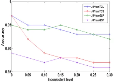
When we consider the cost of different mis-classifications, it is required to compute the four performance metrics mentioned in section IV from the confusion matrix. The TN rate, that can be considered as FP rate (for TN rate =1-FP rate) with different inconsistent level is shown in Figure 3. Form the figure, it can be seen that J-PrismGLP performs best among the four rule-generating strategies, and in addition it also shows the best robustness with inconsistent data.

Figure 2. Accuracy with inconsistent data

Figure 3. TN rate with inconsistent data

Figure 4. FN rate with inconsistent data

However, in cost-sensitive classification, different misclassifications may have different cost. For example, as mentioned in the introduction, the false negative rate may be more important than the false positive rate. Thus, when the FN rate is considered with inconsistent data, the performance is shown in Figure 4. Form the figure, it can be seen that J-PrismGLP does not perform as expected. In

fact, it performs worst among the four rule-generating strategies.

Finally, it is always not enough to investigate classifiers’ performance only based on one metrics, especially in cost-sensitive classification. Just as mentioned in section IV, we need 2D metrics, ROC Graphs, see Figure 5. From the figure, it can be seen that, considering about both TP rate and FP rate, J-PrismTCL performs best among the four rule-generating strategies, and more importantly, it also have the best robustness with inconsistent data.

Figure 5. ROC Graphs with inconsistent data

As presented above, we can easily come to a conclu-sion that in cost-sensitive classification, especially with inconsistent data, one single learning algorithm may often lead to an inherent bias. Thus, to achieve good cost-sensitive classification performance, we should turn to ensemble of classifiers for help in the inconsistent data settings.

VI. CONCLUSIONS

In this paper, we have two main contributions. Firstly, two novel rule-generating strategies are proposed in this paper apart from the previous two main variations of Prism. Thus a completed framework Prism rule-generating strategy has been established. Secondly, the four different Prism rule-generating strategies are used to examine the influence of inconsistent data on cost-sensitive classification, which is an empirical comparative study with experiments on UCI datasets. The most important result of our study is that only one Prism classifier is not enough for a practical cost-sensitive application, especially in inconsistent data setting. For instance, in our experiment, when investigating with false positive rate under different inconsistent level, J-PrismGLP perform well, and has a good robustness; while when investigating with false negative rate, J-PrismGLP does not perform well, in fact it performs worst, comparing with others.

ACKNOWLEDGMENT

This work is supported by the National Natural Science Foundation of China, No.70971134 and No.71371184.

REFERENCES

[1] Lomax, Susan, and Sunil Vadera. "A survey of

cost-sensitive decision tree induction algorithms." ACM

Computing Surveys (CSUR) 45.2 (2013): 16.

[2] Ontañón, Santiago, and Enric Plaza. "Multiagent inductive

learning: an argumentation-based approach." Proceedings

of the 27th International Conference on Machine Learning (ICML-10). 2010.

[3] Dai, Jianhua, et al. "Decision rule mining using

classification consistency rate." Knowledge-Based

Systems 43 (2013): 95-102.

[4] Zadrozny, Bianca, John Langford, and Naoki Abe.

"Cost-sensitive learning by cost-proportionate example

weighting." Data Mining, 2003. ICDM 2003. Third IEEE

International Conference on. IEEE, 2003.

[5] Zhou, Zhi-Hua, and Xu-Ying Liu. "Training cost-sensitive

neural networks with methods addressing the class

imbalance problem." Knowledge and Data Engineering,

IEEE Transactions on 18.1 (2006): 63-77.

[6] Quinlan, John Ross. C4. 5: programs for machine learning.

Vol. 1. Morgan kaufmann, 1993.

[7] Witten, Ian H., and Eibe Frank. Data Mining: Practical

machine learning tools and techniques. Morgan Kaufmann, 2005.

[8] Stahl, Frederic, and Max Bramer. "Computationally

efficient induction of classification rules with the PMCRI

and J-PMCRI frameworks." Knowledge-Based Systems 35

(2012): 49-63.

[9] Kaufman, Kenneth A., and Ryszard S. Michalski.

"Learning from inconsistent and noisy data: the AQ18

approach." Foundations of Intelligent Systems. Springer

Berlin Heidelberg, 1999. 411-419.

[10]Lomax, Susan, and Sunil Vadera. "An empirical

comparison of cost‐_{sensitive decision tree induction}

algorithms." Expert Systems 28.3 (2011): 227-268.

[11]Bramer, Max. "An information-theoretic approach to the

pre-pruning of classification rules." Intelligent information

processing. Springer US, 2002. 201-212.

[12]Stahl, Frederic, and Max Bramer. "Jmax-pruning: A

facility for the information theoretic pruning of modular

classification rules." Knowledge-Based Systems 29 (2012):

12-19.

[13]Cendrowska, Jadzia. "PRISM: An algorithm for inducing

modular rules."International Journal of Man-Machine

Studies 27.4 (1987): 349-370.

[14]Stahl, Frederic, Max Bramer, and Mo Adda. "J-PMCRI: A

methodology for inducing pre-pruned modular

classification rules." Artificial intelligence in theory and

practice III. Springer Berlin Heidelberg, 2010. 47-56.

[15]Smyth, Padhraic, and Rodney M. Goodman. "An

information theoretic approach to rule induction from

databases." Knowledge and Data Engineering, IEEE

Transactions on 4.4 (1992): 301-316.

[16]Provost, Foster, and Tom Fawcett. "Robust classification

for imprecise environments." Machine Learning 42.3

(2001): 203-231.

[17]Frank, Eibe, et al. "Weka-a machine learning workbench

for data mining."Data Mining and Knowledge Discovery Handbook. Springer US, 2010. 1269-1277.

[18]Blake, C. L., & Merz, C. J. (1998). UCI repository of

machine learning databases. http://www.ics.uci.edu/ ~mlearn/MLRepository.html. Accessed 12 June 2012.

[19]Bramer, Max. "Automatic induction of classification rules

from examples using N-Prism." Research and development in intelligent systems XVI. Springer London, 2000. 99-121.

Zhiyong Hao is a Ph.D candidate in College of Information

System and Management, National University of Defense Technology, and his major interest is inductive learning and data mining.

Li Yao is a professor in College of Information System and

Management, National University of Defense Technology, and her major interest is artificial intelligence.

Yanjuan Wang is a Ph.D candidate in College of Information