Modeling and Forecasting Corporate Default Counts Using Hidden Markov Model



Abstract—In this paper, a Hidden Markov Model is employed to fit global, U.S. and European annual corporate default counts. The Expectation-Maximization algorithm is applied to calibrate all parameters while the standard errors of the estimated parameters are conducted by Monte Carlo method. Parametric bootstraps are used to compute the nonlinear forecasts. The empirical results show that the Hidden Markov model is useful in distinguishing the periods of expansion from the periods of recession (relative to the points identified by the NBER). Moreover, it obtains relatively satisfactory forecasts especially in capturing the state switching while incorporating more original observations.

Index Terms—Corporate default counts, expectation-maximization algorithm, hidden Markov model, parametric bootstrap.

I. INTRODUCTION

The issue regarding estimating potential risk levels and forecasting default events of financial assets has increasingly became the interest of many financial, economic, and mathematical researchers in contemporary society. Previously, due to the achievement of Moody [1], the Binomial Expansion Technique (BET) was created to estimate the expected loss of collateralized bond and loan obligations (CBOs and CLOs). However, it is ideal that there exists a pure binomial distribution with independent defaults. With the introduction of diversity score which is used to distinguish a smaller portfolio of independent and homogenous financial assets, it is easier to assume that all these financial assets (bonds and loans) have the same default probability and default independently, resulting in the binominal distribution regarding the quantity of observed default events in single time stage. More importantly, as mentioned by Düllmann [2], some shortages of BET method can be optimized to some extent by the model created by Davis and Lo [3]. In particular, it was related to infectious defaults which increase the default risk of other financial assets. There are two types of risk (normal risk and enhanced risk, respectively), and the latter risk level is enhanced by multiplying infectious factor k. In this case, the similar approach named Hidden Markov Model will be used to detect risk periods in the economy, and related parameters are estimated by Expectation-Maximization algorithm (EM algorithm). More importantly, what this paper pays more attention to concerns corporate default counts forecast, which is different from emphasizing on estimation process and detection of expansion and recession periods in previous

researches. The forecast process is achieved by the parametric bootstrap approach according to Tsay [4], which is used to perform the nonlinear forecasts.

The content of this paper is divided into six aspects. Detailed methods or approaches utilized in this article will be included and explained in Section II and the simulation part Section III is to test the effectiveness of parameter estimation. Then imperial analysis in Section IV incorporates some small related aspects, data introduction, for example. Section V sketches the final conclusion, and the further improvement for this paper is offered in Section VI.

II. METHODOLOGY

A. Model Introduction and Description

In this paper, a two-state discrete HMM is used, and two hidden states are normal risk state and enhanced risk state, respectively, denoting as 1 and 2. According to BET published by Moody’s Investors Service [1], in this case, the default counts N in state 1 and 2 follow different binomial distributions with the parameters 𝑃1and 𝑃2, representing the

observed default probabilities in each state.

1 =( ) 1 (1 1)

n N n N

N

P N（ ） P P  (1)

2( ) ( ) 2 (1 2)

n N n N

N

P N  P P  (2)

where n denotes total number of surviving financial assets (bonds or loans) in the market. More specially, the parameter 𝑃2 is obtained by multiplying 𝑃1 with one factor 𝑘 𝑘 ≥ 1 ,

which describes enhanced effect in state 2.

Moreover, besides the number of states s (2 states in this paper) and the observations per state, the parameters of an HMM also include initial state distribution 𝜋 = 𝑃[𝑞1= 𝑆𝑖]

which means the probability regarding the initial observation occurrence in state i, an observation symbol probability distribution 𝐵 = {𝑏𝑗 𝑚 } to represent the probability of

observing m events on state j (two binominal distributions here), and the state transition matrix 𝐴 = {𝑎𝑖𝑗} which

describes the transition probability from state i to state j [5]. More specifically, in our approach, the parameters to describe the constant transition matrix are demonstrated as follows:

(3) where 𝑎11, 𝑎22 represent the probability of retaining in state 1

and 2 respectively. Hence, complete parameters utilized in our two-state HMM are summarized as 𝜆 (𝐴, 𝐵, 𝜋).

Modeling and Forecasting Corporate Default Counts

Using Hidden Markov Model

Lu Li and Jie Cheng

11 12 22 22

1 1

(

)

A



B. Parameter Estimation

Given the real observation sequence 𝑂 = 𝑂1𝑂2⋯ ⋯ 𝑂𝑇,

the challenges are to estimate HMM parameters (𝐴, 𝐵, 𝑘) and maximize 𝑃(𝑂|𝜆). In 1989, Rabiner recommended one efficient method named EM algorithm to cope with problems, which is utilized to calculate the maximum likelihood value when there is unobserved variables [5]. In forward-backward procedure, there are two separate variables containing forward variable 𝛼𝑡(𝑖) and backward variable 𝛽𝑡 𝑖 . In

detail, 𝑃(𝑂1𝑂2⋯ 𝑂𝑡, 𝑞𝑡 = 𝑆𝑖|𝜆) can be defined as 𝛼𝑡(𝑖)

which represents given 𝜆, the probability of the partial observation sequence when reaching state 𝑆𝑖 at time t.

Similarly, backward variable

𝛽𝑡 𝑖 = 𝑃(𝑂𝑡+1𝑂𝑡+2⋯ 𝑂𝑇, 𝑞𝑡 = 𝑆𝑖denotes the probability of

the rest observation sequence from t+1 to the final after arriving in state 𝑆𝑖 at time t with given model parameters 𝜆.

In order to compute the probability of arriving state 𝑆𝑖 at time t (𝛾𝑡(𝑖)) and transition probability 𝑎𝑖𝑗 from state 𝑆𝑖 at time t

to state 𝑆𝑗 at time t+1 (𝜉𝑡(𝑖𝑗)), they can be defined in the

following form:

1

( ) ( ) ( )

( ) ( )

t t

t s

t t

t

a i i

i

a i i

 

 





1 1

1 1

1 1

( ) ( ( )

( )

( ) ( ( )

t ij j t t t s s

t ij j t t i j

a i a b o i ij

a i a b o i 





     



 

）

）

(5)

C. Forecasts Based on HMM (Parametric Bootstrap)

Unlike the non-parametric bootstrap, the parametric bootstrap is used to draw samples from a distribution formed from a sample set by a model [6]. In this case, nonlinear forecasts are calculated by the parametric bootstrap. Referring to Tsay [4], the values of 𝑥𝑇+1, 𝑥𝑇+2⋯ 𝑥𝑇+𝑙 are

computed by drawing new realizations from specified distribution of the model if estimated parameters are given, where T and 𝑙 (𝑙 > 0) represent the forecast origin and the forecast horizon, respectively. Additionally, by the model, the original observations, the forecast of 𝑥𝑇+1, 𝑥𝑇+2⋯ 𝑥𝑇+𝑙−1and repeating the procedure (M times), M realizations of 𝑥𝑇+𝑙 can be obtained, and then the forecast

of 𝑥𝑇+𝑙 is regarded as the average of M values drawn before.

In this paper, the forecasting process works in the following steps.

1) Start from forecast origin T and the record before T is the first data set to forecast.

2) Perform one-step ahead forecast. In detail, the start point is to calculate the expected smoothed probabilities in T+1 for each risk level ( 𝛾𝑇+1 1 and 𝛾𝑇+1 2 )

given estimated parameters generated from all available data before T. After that, it is essential to randomly draw the default counts from two risk levels and compute the expectation of default count in T+1 by multiplying the 𝛾𝑇+1 1 and 𝛾𝑇+1 2 respectively. By reduplicative

M realizations (1000 in this trial), the forecasting default count in 𝑇 + 1 is the sample average of 1000 expected default counts calculated before. The general forecast process is calculated below, assuming 𝑋𝑇+𝑙𝑗 1 𝑎𝑛𝑑 𝑋𝑇+𝑙𝑗 2 ( 𝑗 = 1 ⋯ 𝑀, 𝑙 > 0) are j

realization for 𝑇 + 𝑙 drew from state 1 and 2 at j times:

𝛾𝑇+𝑙 1 = 𝛾𝑇+𝑙−1 1 ∗ 𝑎11+ 𝛾𝑇+𝑙 2 ∗ 𝑎21 (6)

𝛾𝑇+𝑙 2 = 𝛾𝑇+𝑙−1 1 ∗ 𝑎12+ 𝛾𝑇+𝑙 2 ∗ 𝑎22 (7) 𝑋_𝑇+𝑙𝑗 = 𝑋_𝑇+𝑙𝑗 1 ∗ 𝛾𝑇+𝑙 1 + 𝑋𝑇+𝑙𝑗 2 ∗ 𝛾𝑇+𝑙 2 𝑗 = 1 ⋯ 𝑀 (8)

𝑋𝑇+𝑙 =_𝑀1 𝑀𝑗 =1𝑋𝑇+𝑙𝑗 𝑗 = 1 ⋯ 𝑀 (9)

3) Incorporate one more real default count each time according to the order. The next is to re-estimate related parameters for each data set and repeat forecasting process until all the data are utilized.

Data length in varied regions for forecast is different. The forecast origin for global default counts is T=81 covering the period 1920-2000. Due to the limited data collected about U.S. and Europe, their forecast origins are quite shorter than globe’s (T=29 from1981 to 2009 and T=24 from 1986 to2009, respectively).

D. Covariance Matrix

The standard errors of the estimated parameters (𝑎11, 𝑎22, 𝑃1, 𝑘) are computed by Monte Carlo Method,

which is implemented in the Matlab. In particular, the square root of the values on the diagonal of the covariance matrix concerned is the standard errors of the estimated parameters mentioned before.

The initial step is to generate an observation sequence by prior estimated EM estimators, and repeat this process t times. Next, for each generated sequence, we need to re-estimate parameters (𝑎11, 𝑎22, 𝑃1, 𝑘). Finally, the covariance matrix is

computed below:

C =_𝑡−11 𝑡 𝜃𝑖− 𝜃 ′∙ 𝜃𝑖− 𝜃

𝑖=1 (10)

𝜃 =1_𝑡 𝑡 𝜃

𝑖=1 (11)

where 𝜃 is a vector containing four estimated parameters for each generation.

TABLEI:SIMULATION RESULTS

III. SIMULATION RESULTS

and applied in the EM algorithm. The detailed results are demonstrated in the Table I below, which satisfyingly agrees with the true parameters and supports the effectiveness of parameter estimation. (The brackets here represent the standard errors regarding corresponding estimated parameters)

Fig. 1. Simulated default counts, simulated and estimated risk periods for 1st

set of initial parameters. The solid bar demonstrates risk level in state 2. Hence, the algorithm is satisfying to detect enhanced risk periods.

IV. IMPERIAL ANALYSIS

A. Data Description

The data sources used in this paper consist of Moody’s and Standard & Poor’s annual default studies.

The global data are extracted from Exhibit 16 and Exhibit 30 of Moody’s annual default study [9] which include the number of annual global cooperate issuer default events and annual issuer-weighted corporate default rates from 1920 to 2012. Here we just use actual global default counts from 1920 to 2000 to perform estimation, and the rest data started from 2001 will be applied to forecast. In particular, it should be noticed that all the default counts in Moody’s report only cover Moody’s all-rated cooperate issuers.

As for Europe default counts, it covers the period 1986-2012 in this paper. European default rates are collected from Exhibit 17 of Moody’s European Corporate Default and Recovery Rates [10], and corresponding default counts come from Moody’s annual default study (Excel data), Exhibit 18 [11].

The United States default counts derive from The Standard & Poor’s annual U.S. corporate default studies Table I, covering U.S. default counts from 1981 to 2012 [12]. Meanwhile, these tables also offer corresponding annual default rate.

Additionally, U.S. and European default counts ranging from 1981 to 2009 are used to perform the estimation process and the forecast point begins in 2010, due to the short data length provided by Moody’s and Standard & Poor’s annual default studies.

Data regarding U.S. business cycle are collected from the National Bureau of Economic Research (NBER) [13], which is plotted in Fig. 3 roughly.

B. Default Definition

The statistical data collected from Moody’s and Standard & Poor’s annual default studies implements different default definitions (the difference is described in the annual U.S. Corporate Default Study And Rating transitions [12] and

Moody’s Rating Symbols and Definitions [14]). Moreover, the definition of issuer-weighted default rate is explained in the appendix of Latin American Corporate Default and Recovery Rates [15]

C. Estimation Results

The global, U.S. and European estimation results are demonstrated in the Table II with standard errors within the brackets.

TABLEII:ESTIMATED RESULTS OF GLOBE U.S., AND EUROPE

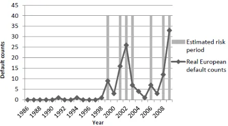
As can be seen from the Table II, the estimation results are quite reliable and stable. Fig. 2- Fig. 4 below demonstrate real observations in globe, U.S. and Europe, along with estimated state switching process. It is clear that the risk states estimated by our model are effective to detect enhanced risk periods, especially in U.S., which capture the real business cycle roughly.

Fig. 2. Real global default counts with estimated risk periods.

Fig. 3. Real U.S. default counts and estimated risk periods along with U.S. business cycle.

D. Forecast results and Analysis

As mentioned in the previous section, the parametric bootstrap will be utilized to predict the global default counts from 2001 to 2012, U.S. and European default counts from 2010 to 2012.

The Fig. 5 below sketches the comparison of observed global default counts with their forecasts from 2001 to 2012. Moreover, the Table III contains two sets of smoothed probabilities in state 1 from 2001 to 2012, one is obtained from applying all available real global default counts from 1920 to 2012, and the other is from rolling estimation process while incorporating a new observation. The detailed data record regarding the comparison between the observed default counts and corresponding forecasts is included in the Table III as well.

Fig. 5. Global default counts and forecasts.

TABLEIII:GLOBAL SMOOTHED PROBABILITIES AND FORECAST RESULTS

While comparing the real global annual default counts with corresponding forecasts from 2001 to 2012, it is interesting to find that there exist large differences between them. Actually, it is reasonable that about 75% of probability that the real default counts in 2001 remains at enhanced risk state, which results from the estimated parameter 𝑎22= 0.75

computed by the data from 1920 to 2000. Our forecast smoothed probabilities are the weighted mean of being in two states, however, the real case is that observations only occur in one state, which results in such a large difference between the real and predicting case. Obviously, the results can be

remedied by incorporating more original data. It is clear that the smoothed probabilities over time obtained by one-step ahead forecast and the parametric bootstrap approach approximately follow the tendency or fluctuation of real global default counts record, which reflects risk state switching.

As for U.S., The similar Fig. 6 and Table IV reflect its default counts, corresponding forecasts and two sets of smoothed probabilities in normal state ranging from 2010 to 2012. It should be noticed that two sets of smoothed probabilities consist of outcomes computed by whole annual U.S. default counts from 1981 to 2012 and one-step ahead forecast process at each rolling step since 2009.

More satisfying results can be obtained from U.S. default observations from 1981 to 2012. In detail, the transition probability 𝑎22 calculated by U.S. data covering the period

1981 - 2009 is 0.75 and the observation in 2009 is estimated at state 2, which lead to 75% of probability that the real default count in 2010 still remains at state 2. More importantly, the forecast smoothed probabilities are the weighted mean of being in two states, however, the real observations only occur in one state, which results in such a large difference between the observed default counts and forecasts. However, with more data, our results will be modified effectively. Obviously, the smoothed probabilities computed by rolling re-estimates process approximately catches the switch between normal and enhanced risk states.

Fig. 6. U.S. default counts and forecasts.

TABLEIV:U.S.SMOOTHED PROBABILITIES AND FORECAST RESULTS

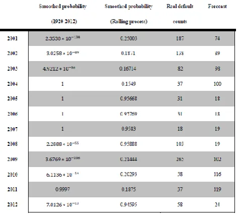
TABLEV:EUROPEAN SMOOTHED PROBABILITIES AND FORECAST RESULTS

The European outcomes are included in the Fig. 7 and Table V.

Although there are large differences between real European default counts and forecasts, what our model estimate can generally catch the state switching, and show that there is a higher probability remaining in recession periods (enhanced risk state) since 2010.

V. CONCLUSION

In this paper, a two-state Hidden Markov Model is used to fit real data in the macro-economy (Globe) and two geographic regions (U.S. and Europe). Related parameters are obtained by EM algorithm. In our case, the U.S. estimated enhanced risk periods capture and follow most recession periods in its real business cycle, which is beneficial for proving the effectiveness of our model. For forecast perspective, the parametric bootstrap is to apply in rolling one-step ahead forecast. Though there are relatively large differences between the real observations and their forecasts, generally, the approach used in this article captures real state switching effectively and forecasts accurately while incorporating more original data.

VI. FURTHER WORKS

Although the model applied in this article can detect enhanced risk periods and capture risk switching, it still needs further works to improve. In detail, firstly, we do not consider cross regional default counts correlation by assuming that they are independent. However, in reality, the global default events in a certain year may trigger the more default events in other geographic regions. Next, the data length is one of our major shortages as well, especially the European default counts only covering from 1986 to 2012, which may cause inaccurate estimation and forecast. Moreover, somehow Markov Chain includes autocorrelation function (ACF), where the next observation depends only on the current observation. There is one alternative approach named integer-valued autoregressive model (INAR) introduced by McKenzie, Alzaid and Al-osh [16], which may improve our method, because we find the significant ACF at lag 1, 2, and 3 while applying global default counts from 1920-2000.

ACKNOWLEDGMENT

Firstly, Lu Li would like to express thanks to Xi’an

Jiaotong-Liverpool University (XJTLU) and XJTLU Summer Undergraduate Research Fellowship for funding and assisting in our project. Then it is very grateful to the Department of Mathematical Sciences in XJTLU for offering this precious opportunity to do this research.

REFERENCES

[1] Moody’s Investors Service, “The binomial expansion method applied to CBO/ CLO analysis,” New York: Moody’s, 1996.

[2] K. Düllmann. (2006). Measuring business sector concentration by an infection model. Germany: Deutsche Bundesbank. [Online]. Available: http://www.fbv.kit.edu/symposium/10th/papers/Duellmann%20-%20 Measuring%20Business%20Sector%20Concentration%20by%20an% 20Infection%20Model.pdf

[3] M. Davis and V. Lo, “Modeling default correlation in bond portfolios,” in Mastering Risk, Applications, London: Pearson Education, vol. 2, pp. 141-151, 2001.

[4] R. S. Tsay, Analysis of Financial Time Series,2nd _{ed. Canada: John}

Wiley & Sons, INC, pp. 192, 2005.

[5] L. Rabiner, “A tutorial on hidden Markov models and selected applications in speech recognition,” Proceedings of the IEEE, vol. 77, pp. 257-286, 1989.

[6] P. V. Heijden, H. Hart, and J. Dessens, “A parametric bootstrap procedure to perform statistical tests in a LCA of anti-social behavior,”

Journal of Educational and Behavioral Statistics, pp. 196-208, 1997. [7] G. Giampieri, M. Davis, and M. Crowder, “A hidden Markov model of

default interaction,” Quantitative Finance, vol. 5, pp. 27-34, 2005. [8] Y. J. Zhu and J. Cheng, “Using hidden Markova model to detect

macro-economic risk level,” Review of Integrative Business and Economics,vol. 2, no. 1, pp. 239-249, 2013.

[9] Moody’s Investors Service, “Annual default study: corporate default and recovery rates, 1920-2012,” New York: Moody’s, 2013. [10] Moody’s Investors Service,“European corporate default and recovery

rates, 1985 – 2012,”New York: Moody’s, 2013.

[11] Moody’s Investors Service. (2013). Annual default study: corporate default and recovery rates, 1920-2012 - Excel data. [Online]. Available: https://www.moodys.com/researchandratings/research-type/default-ra tings-analytics/default-studies/003009000/4294965103/4294966848/0 /0/-/0/-/-/-/-/-/-/-/en/global/pdf/-/rra

[12] Standard& Poor’s. (2013). 2012 Annual U.S. corporate default study and rating transitions. [Online]. Available: https://www.globalcreditportal.com/ratingsdirect/renderArticle.do?arti cleId=1098627&SctArtId=145785&from=CM&nsl_code=LIME [13] National Bureau of Economic Research. (2012). U.S. business cycle

expansion and contractions. [Online]. Available: http://www.nber.org/cycles/cyclesmain.html

[14] Moody’s Investors Service, “Moody’s rating symbols and definition,” New York: Moody’s, 2013

[15] Moody’s Investors Service, “Latin American corporate default and recovery rates, 1990–July 2013,” New York: Moody’s, 2013 [16] M. Kachour and J. F. Yao, “First-order round integer-valued

autoregressive (RINAR (1)) process,” Journal of Time Series Analysis, vol. 30, no. 4, pp. 417-488, 2008