Thermal Simulation of Traction System for High- Speed Train Based on Heat Accumulation

Thermal Simulation of Traction System for

High-Speed Train Based on Heat Accumulation

Huaiyu Xu

Software College Northeastern University, Shenyang, China Email: [email protected]

Jihui Xu, Zhiqiang You, Wenqi Peng, Kunlin Zhang and Jinfeng Xu Software College Northeastern University, Shenyang, China

Email: [email protected]

Abstract—Design of traction system is important to decide the dynamic configuration of high speed EMU. And one of the most important factors that determine the design of traction system is the thermal distribution of IGBT convertors. Thermal simulation of IGBT converter using a two-step methodology (temperature rise and thermal distribution) and its simulation results are presented in this paper [1]. The simulation is based on the combination of an electrical model and a thermal one based on heat accumulation [2] as well as the technique of computer programming [3]. When designers change parameters of these models, the simulating software gets new temperature values and distribution state. So that the simulation can help designers configure the traction system. The modeling results have been checked by operation measured data.

Index Terms—thermal simulation, IGBT converter, heat accumulation, computer programming

I. INTRODUCTION

The traction converter, which is considered to be the heart of the train, determines the properties of the train, such as starting the engine, operation, the high operating speed and so on[4]. Therefore, in order to make the train operate normally and extend the life of the converter, a research on the traction converter is of great importance. As the development of IGBT, it has replaced GTO gradually and has become a first-choice material of converter because of the superior switch characteristics of IGBT [5]. The heating component of the traction converter is also called IGBT module. This paper will take CRH2 as an example, and study the temperature rise of the converter.

Temperature is one of the main factors influencing the reliable of power semiconductor. Excess heat can cause failure of semiconductor junction which is sensitive to temperature. For every increase of 2℃ in working

temperature, the reliability of electronic components has a fall of 10% [4]. The temperature rise problem has been studied for many years. Early investigators used steady-state models to calculate the junction temperatures of semiconductor. However, temperature rises of EMU are continuous processes. Early investigators didn’t consider the accumulation of heat which affects the temperature.

For example, Robert and Rohinton solved the temperature drop between a transistor junction and the

base of a silicon chip for boundary conditions which approximate a set of operating conditions. However, they calculate the temperature in steady-state which is more likely a performance index of the semiconductor chip but not the runtime state of the chip. [6] There are many studies based on and improved Robert and Rohinton's study like Zhang Mingyuan and Shen Jianqing's "Calculation Method of a Fast Power Loss" which also calculate the losses under steady-state.

With respect to thermal simulation of semiconductor chips, Ellison studied the 3-D heat conduction equation in rectangular coordinates with Newtonian cooling of both the surface source plane and the opposing external surface plane by a Fourier series solution in early 1970s. [14] Lee's study which includes 1-D internal conduction and external resistances shows his theory is more complete to prove that the total resistance from source to ambient is the sum of spreading. [12] Nelson and Sayers compare 2-D planar and axisymmetric spreading resistances with three-dimensional (3-D) resistances. [13]

This paper calculates the temperature rise of the converter which is regarded as a semiconductor material based on heat accumulation. Firstly, the converter is considered as a whole, according to its equivalent resistance and current, and its instantaneous losses are calculated, then temperature rise are also calculated based on heat accumulation. IGBT module is the main heating element in converter, so identify it as the heating source and establish the thermal model of the whole converter. Then, according to the Maximum Thermal Spreading Resistance algorithm, calculate the heat distribution of the whole converter [3]. Finally, by using the technique of computer simulation, program and show the instantaneous temperature distribution of the converter.

II. MODELING METHODOLOGY

In order to calculate the temperature of converters, it’s important to build models usable for electro-thermal simulation. The resistance-capacitance model is defined taking the temperature dependence of equivalent resistance and capacitance into account. In other word, this model takes one converter as a whole entity. On the other hand, the 2-D and 3-D thermal model is based on the physical and geometrical description of the converters.

A. Resistance-Capacitance Model

This model takes the converter as a whole entity, and analyzes the electrical properties. The equivalent circuit diagram is shown in Fig. 1.

First, we should calculate the energy losses of the component. As we analysis, the losses conclude two parts: IGBT energy losses (PIGBT) and two-electrode valve

energy losses (PD). We define the whole losses as P [7].

D IGBT

P

=

P

+

P

Also, PIGBT and PD both conclude two parts: on-state

energy losses and circuit changer energy losses.

IGBT SS SW

P

=

P

+

P

D DC rr

P

=

P

+

P

Detail processes of calculation refer to formula I-IV in appendix B. Then, the temperature rises are obtained using the results of energy losses based on heat accumulation.

Based on the law of conservation of energy, we get the differential equation.

dt

S

cGd

Pdt

=

τ

+

α

τ

Pdt

--energy losses of the whole module in time

dt

.

τ

cGd

--accumulation heat. G is the weight of module. c is the specific heat. And

d

τ

is the temperature rise in time

dt

.

dt

S

τ

α

--heat release in time

dt

.

α

is coefficient of heat transfer. S is the area.

To solve the equation, we get another equation about temperature rise (

τ

).

cG St cG St

e

S

e

P

(

1

α /

)

/

α

τ

₀ α /

τ

₌

₋

−

₊

−

In the equation, we assign 0 to

τ

₀ and a fixed time variable (

Δ

t

) to t. So the temperature rise is determined by the constant losses (

P

) and accumulation of heat (

cG

).

Figure 1. Equivalent circuit diagram of the converter.

B. 2-D Thermal Model

As we obtain the IGBT junction temperature, the 2-D thermal model is established based on the Maximum Thermal Spreading Resistance algorithm proposed by Ellison [2] [5] [8]. In the model, we take the IGBT as the heat source. As shown in Figure 2 is finite plate model for a source with planar area △x△y and an opposing surface

of area ab. So we can get the formula of temperature distribution from Ellison’s paper [1]. Then, we can calculate the temperature of any point on the plate just taking the coordinates as the variables (z = 0).

) cos( ) cos( ) cos( ) 2 1 ( ) cos( ) 2 1 ( ) 4 1 ( ) , , ( 1 1 0 1 m 0 1 00 _b y m a x l b y m a x l z y x T m lm l m l l π π π π

_ψ

_ψ

ψ

ψ

∑ ∑ ∑∑∞ = ∞ = ∞ = ∞ = + + + =

Figure 2. Plate model for a converter with heat source area △x△y. Detail processes of derivation of formula and nomenclature please refer to Ellison’s paper. After calculation, the accuracy of 5% has been achieved for both the simulation results and the measured values. C. 3-D Thermal Model

The 3-D model is the same as 2-D model in which we evaluate z = 0. In the 3-D model z axis ranges from 0 to 6cm and the heat source is a rectangular cube instead. An overhead view of the 3-D model is the same with figure 2. With the 3-D thermal simulation of the convertor, we can see the distribution of the temperature from an overhead view, a front view and a side view which can show the distribution roundly and obviously.

III. COMPUTER SIMULATION

As we know the performance of converters is very important in the high-speed train running. Computer simulation of converters, on one hand, can show the thermal property of the component under different current, such as energy losses and junction temperature. On the other hand, it can display the temperature distribution of the extracted plate intuitively. As a result, designers can change parameters by the software to look over different results which help to design of train hauling capacity and dynamic configuration.

A. Design Curves

The axes curves graph is designed based on the resistance-capacitance model. Firstly, the paper draws the static characteristic curves of the IGBT convertors. These curves are aimed to present the steady-off temperature variation during continuous variation of current.

Example:

As we mentioned above, in this paper we take CRH2 as the example. Table I provides the electrical system parameters of the coach. And the type of IGBT used is FF600R17KE3.

TABLE I. ELECTRICAL SYSTEM PARAMETERS OF THE COACH

Vdc Icp Fsw M Cos Ta Tz Thsa

After calculation and simulation we get the curves shown in Figure 3 and Figure 4.

Figure 3. Converter’s energy losses under continuous variations of current.

Figure 4. Converter’s energy losses under continuous variations of current.

By these curves graph, we can observe and analyze converter’s thermal characters under different currents, so that they can guide the design of the train’s dynamic configuration.

Secondly, in order to simulate the temperature rise of the whole process of train running, the paper draws continuous changed curves.

Example:

Also, take CRH2 as the example. Input the running parameters of CRH2 between Peking and Shenyang. We get the continuous temperature change curve. In this model, value of

Δ

t

is 10ms,

α

is 2, and c is 0.168. The first ten second running simulation is shown in figure 5.

Figure 5. Continuous temperature change of first 10 seconds.

The calculation of this curve is based on heat accumulation. Compared to former model of steady-state, this model considers the effects of former state to continuous states which is nearer to the actual situation.

B. Draw 2-D Simulation Pictures

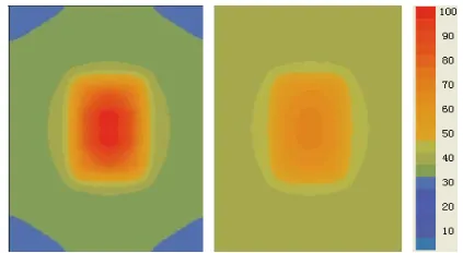
The 2-D simulation pictures are designed to show the temperature distribution of the converter. Just mentioned above we calculate the distribution based on the Maximum Thermal Spreading Resistance algorithm, and take the IGBT as the heat source. In order to calculate the steady-state temperature distribution, the program first gets the current and calculates the temperature distribution under this current. Then the program generates a graph based on a certain scale to the real converter and maps certain points’ temperature to the graph. Also the program should generate chromatogram map matching different temperature ranges, so that the temperature calculated above can find their own colors in this map. Finally, the program colors the graph and shows it to the monitor. Figure 6 shows temperature distribution under different currents. Input parameters are shown in Table II.

TABLE II. INPUTPARAMETERSOFTHE2-DSIMULATION α ₌ β Biot·τ Nx = Ny R-Figure Icp

0.1 10-3 20 8 50

0.1 10-3 20 8 80

During the process of coloring the graph, we use the method of pointer image processing. First we get the pointer value of a certain point on the graph. Then, we get the temperature of the point by mapping to the real entity, so we get the color as well as the R, G, and B values. Finally, assign the R, G, and B values to the pointer [11].

Figure 6. The temperature distribution of first picture is under low current about 20A. Second one is under current about 50A, and the third

one is under 80A. The last picture is the map of color to temperature.

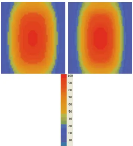
Another set of test data are shown in table III.

TABLE III. INPUTPARAMETERSOFTHE2-DSIMULATION α ₌ β Biot·τ Nx = Ny R-Figure Icp

Figure 7. Results of test data in figure III.

By these thermal simulation pictures, we can observe the temperature distribution of the converter, so that it can guide the design of forced-air cooling equipment.

C. Draw 3-D Simulation Pictures

Based on the 3-D Thermal Model in II-C we program to show the 3-D thermal distribution of the convertor. The process of this simulation is mostly like the 2-D simulation. Firstly, establish the x/y/z axis system. Then, calculate the temperature of T(x,y,z) by the formula in appendix B. Finally, convert the temperature to colors based on the map and show them.

The paper used a set of test data shown in table IV to verify the program.

TABLE IV. INPUTPARAMETERSOFTHE3-DSIMULATION α ₌ β Biot·τ Nx = Ny R-Figure Icp

0.1 10-3 20 8 80 0.1 10-3 120 8 200 The 3-D simulation program is designed to show the temperature distribution of the convertor in different views. Result pictures of the first row of test data are shown as below. Figure 8 simulates the distribution seen from the side-overhead view, and figure 9 is seen from the front view. Also there is an overhead view which is shown in the second picture of figure 6.

Figure 8. Side-overhead view of thermal simulation.

Figure 9. Front view of thermal simulation.

Result pictures of the first row of test data are shown in figure 10 and 11, and the front view is shown in the second picture of figure 7.

Figure 10. Side-overhead view of thermal simulation.

Figure 11. Front view of thermal simulation.

IV. SOFTWARE DESIGN

The process of calculation is carried out in the following way: Electrical parameters of the train and IGBT parameters obtained from the equipment provider are exported in the database. Then these parameters are used as the inputs in the resistance-capacitance model. Next, values of energy losses are obtained, which are also used as the inputs of the calculation of temperature of the converter. Temperature of extracted entity is obtained from the resistance-capacitance model, being the new inputs for the 2-D thermal model as well as the physical and geometrical parameters. Then, we get the thermal distribution of the model based on the Maximum Thermal Spreading Resistance algorithm. At last, we present the temperature distribution by means of computer simulation. In addition, the 2-D thermal model is from the 3-D thermal model which evaluate z = 0. So the paper also adds the 3-D simulation by adding variable z, and presents the 3-D temperature distribution from different views by program.

V. CONCLUSIONS

The paper introduces calculation of converter’s temperature as a whole and its temperature distribution in both 2-D and 3-D. Then program to display temperature under different currents by curves and simulate the thermal distribution of IGBT converter by chromatogram-temperature graph, as well as different views in 3-D. Therefore, this program can provide guidance to the design of train’s dynamic configuration and forced-air cooling equipment.

However, there are still some defects in the work. In the 2-D thermal model, the paper only takes one IGBT into account while there are 6 or more IGBT modules in the converter. Although the paper takes the converter as a 3-D model, it doesn’t take many details into account such as the heat source’s numbers and structures. So in the future, all the IGBT modules will be added into the model considering the stacking heating of different source and there will be a more refined 3-D thermal model to simulate the real runtime state of the convertor.

APPENDIX A NOMENCLATURE AND TEST VALUES

CEsat

V

IGBT saturation voltage drop 2.4(V)

CN

I

IGBT rated current 600(A )

CEN

V

CE terminal voltage 900(V)

dc

V

Dc bus voltage 900(V)

CP

I

Inverter maximum current 707(A)

SW

f

Switching frequency 2000(HZ)

cos

ϕ

Power factor 1

M Modulation ration 1

1 3CN

CE I

V

_{Voltage when 1/3 rated current 1.4(V)}

( )

I on N

E

_{IGBT Opening loss 0.19(J)}

( )

I off N

E

_{IGBT Closing loss 0.22(J)}

( )1₃

I on

E

1

3ICN IGBT Opening loss 0.07(J)

( )1₃

I off

E

1

3ICN IGBT Closing loss 0.08(J)

( )5₃

I on

E

5

3ICN IGBT Opening loss 0.39(J)

( )5₃

I off

E

5

3ICN IGBT Closing loss 0.38(J)

Fsat

V

FWD rated conduction pressure 1.7(V)

1 3CN

F I

V

1

3ICN conduction pressure drop 1.1(V)

( )

D off N

E

_{Rated turn-off loss 0.21(J)}

lead

R

Guide thermal resistance 3e-4(K/W)

Ithcs

R

IGBT thermal contact resistance 0.02(K/W)

Dthcs

R

FWD thermal contact resistance 0.05(K/W)

thsa

R

Atmospheric thermal resistance 0.08(K/W)

Dthjc

R

_{FWD junction resistance 0.06(K/W)}

Ithjc

R

IGBT junction resistance 0.03(K/W)

a

T

free air temperature 40(℃)

APPENDIX B FORMULA I

1 3

3

1

2

CN

2

CEO CEsat

CE I

V

=

V

−

V

CEsat CEO CE CN

V

=

V

+

r

∗

I

···

r

_CE

1 3

1

1

2

3

CN

CEO CE CN

CE I

V

=

V

+

r

′

∗

I

···

r

_CE

′

1

0

3

CP CN

I

I

≤

≤

2

1 cos 1 1 cos

( ) ( )

2 8 2 8 3

SS CEO CP CE CP

M M

P ϕ V I ϕ r I

π π ′

= + ∗ ∗ + + ∗ ∗

1

3

CP CN

I

>

I

2

1 cos 1 cos

( ) ( )

2 8 8 3

SS CEO CP CE CP

M M

P ϕ V I ϕ r I

π π

Formula II

0

≤

I

CP

≤

I

CN

( ) ( )

(

)

( ) ( ) _{( )}1 _{( )}1

3 3 3 1 2 CP CN dc

SW SW I on N I off N I on N I off N

I on I off

CEN CN

I I

V

P f E E E E E E

V I π ⎡ ₋ ⎛ ⎞⎤ = ∗ ∗ ∗⎢ + + ⎜ + − − ⎟⎥ ⎢ ⎝ ⎠⎥ ⎣ ⎦ CP CN

I

≥

I

( ) ( )

(

)

_{( )}5 _{( )}5 ( ) ( )

3 3

3

1

2

CP CN dc

SW SW I on N I off N _{I on I off} I on N I off N

CEN CN

I

I

V

P

f

E

E

E

E

E

E

V

I

π

⎡

−

⎛

⎞

⎤

= ∗

∗

∗

⎢

+

+

⎜

+

−

−

⎟

⎥

⎢

⎝

⎠

⎥

⎣

⎦

Formula III 1 3

3

1

2

CN

2

FO Fsat

F I

V

=

V

−

V

Fsat FO F CN

V

=

V

+ ∗

r

I

···

r

_F

1 3

1

1

2

3

CN

FO F CN

F I

V

=

V

+

r

′

∗

I

···

F

r

′

1

0

3

CP CN

I

I

≤

≤

2

1 cos 1 1 cos

( ) ( )

2 8 2 8 3

DC FO CP F CP

M M

P ϕ V I ϕ r I

π π ′

= − ∗ ∗ + − ∗ ∗

1

3

CP CN

I

>

I

2

1 cos 1 cos

( ) ( )

2 8 8 3

DC FO CP F CP

M M

P ϕ V I ϕ r I

π π

= − ∗ ∗ + − ∗ ∗

Formula IV

( )

1

_*

CP dc

rr SW D off N rr

CN CEN

I

V

P

f

E

P

I

V

π

= ∗

∗

∗

+ Δ

1

0

2

CP CN

I

I

≤

≤

( ) 1

1

rr D off N SW

P

E

f

k

π

Δ =

∗

1

2

I

CN

<

I

CP

<

I

CN

2 CN CP rr SW

I

I

P

f

k

π

−

Δ =

∗

CP CN

I

≥

I

3 CN CP rr SW

I

I

P

f

k

π

−

Δ =

∗

Formula V

[

]

2 2

1 ( 25 )

4 4

CP CP

lead lead lead

I I

P =r ∗ = +

α υ

− °C ∗R ∗

35

25

CP CN

I

I

υ

=

+

∗

Ithcs Dthcs thcs Ithcs Dthcs

R

R

R

R

R

∗

=

+

(

)

(

)

C S thcs IGBT D

S a thsa IGBT D lead

jD C Dthjc D

jI C Ithjc IGBT

T

T

R

P

P

T

T

R

P

P

P

T

T

R

P

T

T

R

P

= +

∗

+

⎧

⎪

_{= +}

_∗

₊

₊

⎪

⎨

₌

₊

_∗

⎪

⎪

₌

₊

_∗

⎩

(

α

=

3.85 10

×

−3

°

C

−1 (Cu))

ACKNOWLEDGMENT

In the paper, we got much help of electric formula and model design from our colleague of Northern Jiao Tong University, thanks.

REFERENCES

[2] Changchun Chi, Yi Wu. “Based 0n Heat Accumulation Over-load Protection Mathematical Model” The third electrician product reliability and electricity contact international meetings, vol. 45, NO. 2, Oct 2009.

[3] Gordon N. Ellison. “Maximum Thermal Spreading Resistance for Rectangular Sources and Plates With Nonunity Aspect Ratios,” IEEE Transactions on Components and Packaging Technologies, vol. 26, NO. 2, June 2003.

[4] Miquel Vellvehi. “Coupled electro-thermal simulation of a DC/DC converter,” Microelectronics Reliability, vol. 47, pp. 2114–2121, April 2006.

[5] KojimaT, YamadaY, CiappaM, ChiavariniM, FichtnerW. “Anove electro-thermal simulation approach to power IGBT modules for automotive traction applications,” R&D Review of Toyota CRDL, vol 39, No. 4, 2004. [6] Lindsted Robert, D.Surty, Rohinton J. “Steady-State

Junction Temperatures of Semiconductor Chips,” IEEE Trans. on E.D. ,Vol. 1, pp. 41-44, 1972.

[7] J. Qian, A. Khan, A. I. Batarseh. “Turn-off switching loss model and analysis of IGBT under different switching operation modes,” Proc. 21st International Conference on Industrial Electronics, Control, and Instrumentation, vol.1, pp. 240 –245, Nov. 1995.

[8] Shoucai Yuan. Introduction of IGBT field effect semiconductor power devices [M]. Science press, 2008, 80-100.

[9] Professional2-Dversion.Tech.Rep.,

PDESolutions,Inc.,Antioch,CA.[Online]. www . pdesolutions . com.

[10] Master of zedGraph. [Online] Available: http://blog.csdn.net/tjvictor/

[11] archive/2006/11/24/1412550.aspx.

[12] Three ways of image processing. [Online] http://www.cnblogs.com/

[13] aipeiyi/archive/2010/07/29/1787846.html.

[14] [12] L. Lee, V. A. S. Song, and K. P. Moran, “Constriction/spreading resistance model for electronics packaging,” in Proc. 4th ASME/JSME Thermal Eng. Joint Conf., vol. 4, Maui, HI, 1995, pp. 199–206.

[15] [13] D. J. Nelson and W. A. Sayers, “A comparison of 2-D planar, axisymmetric and 3-2-D spreading resistances,” in Proc. 8th Annual IEEE Semicond. Thermal Meas. Manag. Symp., Austin, TX, 1992, pp. 62–68.