Space Target Tracking by Variance Detection

Space Target Tracking by Variance Detection

Yunnan Astronomical Observatory/Chinese Academy of Sciences, Kunming, China Email: [email protected], {xyh, lzhl, zhouyu, lyq}@ynao.ac.cn

Tao Huang

University of Chinese Academy of Sciences, Beijing, China Email: [email protected]

Abstract—Detecting and tracking small targets in the aerospace is both a significant and difficult issue for the satellite tracking system. It is fundamentally challenging due to the existence of strong noise in captured images, the few characteristics of spot-like target, the simultaneous multiple targets, the real-time requirements, and so on. To address these challenges, we respectively design the detector and tracker who coordinate with each other. We formulate the detection stage as a two-step problem, which integrates the variance vector detection and 2th variance detection. The pixels of images are projected to the variance subspace of two-dimension. In the first step, the candidate targets are extracted with the optimal threshold achieved by K-means and proposed Weighted Maximum Right Probability, namely WMRP. In the second step, the true targets are checked out by adopting the proposed 2th variance feature and multi-scale threshold. In the tracking stage, the Markov based dynamic model forecasts the probable area of the target in next time which is presented to the variance detector. Then the real location of the target estimated by the detector is transmitted to the tracker to generate the next probable area. Experiments demonstrate the proposed two-step framework can efficiently and rapidly detect the small multiple targets, and the cooperative working of the detector and tracker can satisfy the conventional application of space target tracking.

Index Terms—detection; tracking; space target; 2th variance; multi-scale threshold

I. INTRODUCTION

Space targets detection and recognition refer to the discriminations of space targets types, properties, uses and threats for the purpose of accurately mastering the real-time space situation. The visible imaging devices, such as electronic fence, photometric system, satellite laser ranging system and so on, mainly focus on tracking and measuring satellites and space debris [1]. Since these space targets usually enjoy a long distance of a few hundred kilometers or more from the ground stations, the shape and texture characteristics of space targets are almost drowned and usually present themselves as spots

that occupy only several pixels. Meanwhile, the impacts of atmospheric turbulence and imaging device noise lead to the further difficulties for detection and tracking. In order to address this issue of small target detection and tracking, scholars have proposed various algorithms. Multistage Hypothesizing Testing (MHT) [2] treats a number of candidate trajectories as a tree-structure. The pixels along a trajectory are tested sequentially for a shift in mean intensity using MHT which is designed according to the pre-specified error probabilities. The dynamic programming [3] [4] based algorithm integrates the measurements along possible target trajectories, returning as possible targets those trajectories for which the measurement sum exceeds a given threshold. These two methods mentioned above can be mainly classified into the method of Track-Before-Detect (TBD) [5], which is useful when the image Signal to Noise Ratio (SNR) is very low. But they always encounter with high computation complexity and hard threshold. Meanwhile, the strong target produces disturbance to the weak one greatly. In the area of astronomical photoelectric detection and tracking, due to the effect of atmosphere turbulence, the imaging of space target is always not ideal. Moreover, if the target in the image is very small and weak, the observer and the telescope system attempt to use the techniques of long exposure and defocusing to enable the detectable target to be appearing as a small spot more than 2×2 pixels. For these reasons, the TBD methods are not usually adopted in professional detection device except for the general video Charge Coupled Devices (CCD), and the method of Detect-Before-Track (DBT) is more appropriate for the space detection and tracking. Some algorithms based on background prediction, such as the temporal filter [6] and spatial filter [6], incorporate a prior knowledge of the target and background statistics to enhance the image SNR. Nevertheless, the movement of board platform and the camera self-jitter certainly increase the difficulty of background estimation. Some approaches based on target enhancement have been proposed, such as local entropy [7], high-pass filtering [8], morphology filtering [9] [10], wavelet filtering [11] [12], etc. Local entropy approach deems that the small target leads to the change of local entropy which is served as the detection criterion. High-pass filtering based method suppresses the background to reserve the targets and noise component,

Manuscript received November 30, 2013; revised February 15, 2014; accepted March 1, 2014.

Project supported by the National Natural Science Foundation of China (No.10978025)

and then it screens the targets according to the distribution property of noise. Morphology filtering aims to enhance positively contrasted and isotropic objects with a specified size. However, the size of the structure element is very sensitive for the detection result when the objects are not of the same and fixed sizes. These target enhancement based algorithms all directly treat target and noise as medium-high frequency signals, but in this way they may detect some false targets caused by strong noise. Upon detecting the targets, they need a tracker to estimate the next states and associate these trajectories. The classic tracking algorithm is the Kalman Filter, but it is just appropriate for the situation that the dynamic procedure and measured process are both linear and Gaussian. To overcome this limitation, the Extended Kalman Filter (EKF) [13] is proposed to approximate the nonlinear model to be linear. Some scholars attempt to introduce the Weighted Statistical Linear Regression (WSLR) into the Kalman theory for the purpose of addressing the nonlinear problem better, for example, the Unscented Kalman Filter (UKF) [14] and Central-Difference Kalman Filter (CDKF) [15].

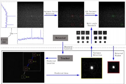
For images of space targets against single background, in this paper, we propose a novel and real-time detection and tracking algorithm that employs the variance vector and 2th variance features. Our algorithm belongs to the DBT method, and it merges the detector and tracker together which coordinate mutually to fulfill the tracking task. Fig.1 is the flowchart of the proposed method,

which integrates the two stages of detection and tracking. In the detection stage, different from the starting point of the algorithms mentioned above, the proposed algorithm projects the two-dimensional image into a variance subspace containing two variance vectors. And they separately extract the singularity parts from row and column variances with the optimal thresholds obtained by the fusion algorithm of the K-means and the proposed Weighted Maximum Right Probability (WMRP). The locations of singular parts in row and column directions can be combined as the positions of candidate targets. In other words, the variances of grayscale intensity in each dimension (row and column) are combined together to detect protuberant targets. Then the feature of 2th variance is employed to single out the true targets with the method of multi-scale threshold. In the tracking stage, we regard the target state as a 3-order Markov process. Thus, the state of the next frame is described by the states of the latest 3 frames, which gives the motion model. With the tracker, the target position of the next frame can be predicted, and the windowed area is transferred to the detector mentioned above. Then another smaller window centered the observed location is added, and the observed location is provided to the tracker to forecast the next location. In this way, the two stages of detection and tracking can be performed iteratively. Note that the proposed method is not designed for the complex circumstance, but to supply a novel and efficient idea for the practical problem. Therefore, we just concentrate on

Figure 1. Procedure diagram of our algorithm. (1) The optimal threshold thM is determinated with the fusion algorithm of K-means and WMRP

through a group of sample images. (2) The target and background blocks of various sizes are employed to construct multi-scale thresholds. (3) For the testing image, the variance vectors in row and column are calculated and the candidate targets are preliminarily detected. (4) The true targets are secondarily checked out within the 2th variance detection. (5) The measured location is transmitted to the tracker to predict the probable area of target with the dynamic model based on Markov theory. (6) The probable area is processed with the method of variance detection. (7) The real location of the

the 2th variance instead of other typical features. If some decoys (CCD smear, star, non-target satellites, non-target debris, etc) appear, the auxiliary features (shape, luminance, velocity, direction, etc) can be jointed with the 2th variance to discriminate the true targets at the secondary judgment, but it is not the focus in this paper. In the rest of this manuscript, section II gives the definition of 2th variance and analysis of its properties, and then section III discusses the process of detection and tracking algorithm. Next, the detection and tracking experiments are demonstrated in section IV. At last, section V has a brief conclusion.

II. 2TH VARIANCE AND PROPERTY

In probability theory and statistics, the variance is one descriptor of probability distribution describing how far the numbers lie from the mean. If a random variable X has the mean μ=E[X], then the variance of X is the covariance of X with itself, given by:

] ) [( )

(_{X =E X−μ} 2

Var . (1)

The 2th row and column variances are proposed on the basics of row and column variances. To simplify the discussion, only the row variances and 2th row variance are discussed. Provided that the size of the acquired image is M×Nand the grayscale of pixel is f(i,j). The row variances can be represented by Vr=[V_r(j)], and

∑

=

−

= M

i

rj

r f i j

M j V

1

2 ] ) , ( [ 1 )

( μ , (2)

∑

=

≤ ≤

= M

i

rj f i j j N

M ₁ (, ) 1

1

μ . (3)

Note that row variances are a vector containing the variances of all the columns of image. Then the 2th row variance, which is the variance of all the elements in the row variance vector Vr, is represented by

∑

= −

= N

j

r r

r V j

N V

1

2

2 1 [ ( ) μ ] , (4)

∑

=

= N

j r

r V j

N 1

) ( 1

μ . (5) Given the equations of the variances above, we need to discuss the property of the proposed feature named 2th variance. A useful feature in a certain range can magnify the differences among the various categories, while it also can reduce the differences of the similar objects. In general, space target image is composed of the dark deep space background, the small spot-like targets as well as the noise points introduced by imaging equipment (noise, bad column and hot pixels) and space environment (nebulae, galaxy and cosmic ray) [16]. Considering that the small space targets are featureless and the background of starry sky is not complex, we just emphasize the impacts of these three aspects (location, daylight and

noise) to the 2th variance but not caring about the affine invariance and rotation invariant. Then we take 60 64×64

image blocks to test, the 20th, 21th, 29th, 30th and 60th of which are target blocks.

1.From (2) and (4), the change of target position just affects the variance vector, but it has little effect on the 2th variance.

2. When the light intensity increases or decreases uniformly, the variance vector and the 2th variance maintain their values theoretically. But actually it needs to ensure the grayscale of each pixel within the range of 0 to 255. As shown as Fig.2 (a), only the 2th variance of target block has remarkable variation when increasing the grayscale of image with the amplitude limiting processing. Meanwhile, the decrement of 2th variance becomes larger as the increment of grayscale becomes larger. In contrast, the 2th variance of the target block may rise if the luminance is weakened.

3. It is crucial that the 2th variance is not easily interfered by noises. Since the average grayscale of background block is always smaller than the target block, the background block is more susceptible to the noise. In other words, the 2th variance of background block will vary greater than the target block. Fig.2 (b)-(d) show the change rate of 2th variance when adding those 3 kinds of noises, and they demonstrate that the target blocks maintain similar values as before regardless of the Gaussian or salt & pepper noise. Note that all numerical parameters in the sub-figure are normalized, which correspond to the adding noise operations with intensities ranging from 0 to 1.

III. DETECTION AND TRACKING ALGORITHM

According to the advantages of 2th variance and variance vector for the target detection against starry sky background, we propose the detection algorithm for online detection containing two steps: variance vector

Figure 2. Properties of 2th variance. (a) Increasing brightness; (b) Salt and pepper noise; (c) Gaussian noise of zero-mean; (d) Gaussian noise of

0.25 mean. There are 60 64×_{64 images, the 20th, 21th, 29th, 30th and}

60th of which are target blocks. In (a), some value is added to the grayscales of all pixels with the processing of amplitude limiting, that is,

the grayscale should not exceed 255. In (b)-(d), the various types of the noises with different intensities are added to the images to study the

detection and 2th variance detection. Variance vector detection achieves the locations of candidate targets, while 2th variance detection singles out the true targets. Then we build the dynamic model of target and predict the probable area with the Markov theory which will be provided to the detector mentioned above. Afterwards, the true position of the target estimated by the detector is transmitted to the tracker again. It is emphasized that the sequential images have been preprocessed with the filter for the purpose of suppressing the undulate background. A. Variance Vector Detection

To solve the high computational complexity problem of the block based method, we directly calculate the row variances and column variances in the whole image. The variance of the column with target pixels is always larger than the background column, thus how to determine the suitable threshold to discriminate the target columns is crucial. Considering the size of target maybe several pixels but not large, the variances of target columns can be regarded as the singular points in the sequence points of row variances. Since every image has its specificity, it is not wise to set a fixed threshold, but the self-adaptive threshold which may perform better is usually time-consuming. Therefore, we propose the hybrid training algorithm of K-means learning and WMRP criterion to balance the performance and calculation according to an abundant sample library which can be updated periodically.

Given many target images of the same size, we can extract all the variance vectors to build a training set

} ... ,

{ (1) (2) (m)

x x

x . It can be treated as a problem of unsupervised two-class classification. The variances of target columns and non-target columns both follow Gaussian distribution approximately, thus the off-line training algorithm is described as follows:

1. Initialize cluster centroids _∈ℜn

2 1,μ

μ randomly.

2.Repeat until μj convergences, i=1,2...m, j=1,2:

2 ) ( )

( _argmin

j i j

i _x

c = −μ , (6)

∑

∑

μ . (7)

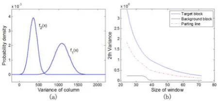
3. Estimate the probability density functions of f1(x)

and f₂(x) for the target and background columns with the Gaussian model as shown as Fig.3 (a).

4. Maximize the normalized right detection probability )

(th

Pd depending on the threshold variable th, and then the optimal threshold is

) ( max

arg P th

th _d

th

M = , (8)

dx x f dx x f th P th th

d ( )

1 ) ( 1 1 )

(

∫

∫

∞ + + + = α α

α , (9)

where the indicator function 1{⋅} takes on a value of 1 if its argument is true, and 0 otherwise. Due to the lower cost of false-alarm than that of leaking detection, the weight factor α always takes below 1. Some false target columns can be checked by the 2th variance method at the secondary extraction. If th is taken as a suitable value in the middle domain,Pd(th) will approach 1. Meanwhile, if th is set to be some value of two sides, P_d(th) will be a little larger than 1(1+α) or α +(1 α). Thus the objective function usually has a maximum value, and the corresponding optimal threshold thM can be solved by the derivation approach.

In the online discrimination, having detected the target columns with the optimal threshold, the corresponding indexes for the local maximum variances of target columns can be taken as the preliminary X coordinate positions of targets. They are expressed by

{

}

possible locations in X coordinate. Furthermore, the permutation of the coordinate positions for the target rows and columns can be deemed as two dimension locations of the possible targets, which are represented as

) , (Xrmi Ycmj .

B. 2th Variance Detection

For each candidate target detected in the variance vector detection, a window centered (Xrmi,Ycmj) is added and the 2th variance of this block is calculated. Then we determine the threshold which is used to decide whether the candidate block is target block or not. However, for one same target, the 2th variances of blocks are dissimilar if the sizes of the added windows are different, which causes the difficulty of determining the threshold. It can be seen in Fig.3 (b) that the 2th variance of target block slides down rapidly as the window size increases, while the 2th variance of background block changes slowly. This indicates that it is impossible to wholly separate the target and background block with a constant threshold. To achieve a more accurate decision, we propose the method of multi-scale threshold which can adapt the variant sizes of windows. Firstly, P typical sizes between 16×16 and 64×64 are selected as S={s1...sp...sP}.

Figure 3. Illustrative graphs for our algorithm. (a) Gaussian distribution fitting; (b) Multi-scale thresholds. f1(x) and f2(x) are the fitting curves for the target and background columns, as shown as (a). The variances of target columns mainly distribute in the nearby area of 1100, while the variances of background columns mainly distribute in the neighbor area of 350. It is shown in (b) that the 2th variances of image blocks are also different if the sizes of the added windows are different. The dotted line

The smaller box is suitable for the denser multiple targets, while the larger box is appropriate for the sparser multiple targets. Then lots of sample blocks in diverse sizes are collected to establish the sample library

} ,

{ t b

I I

I= , where {₁... ... Pt} t p t t I I I

I = and {₁... ... Pb} b p b b I I I

I = .

Note that the superscript t and b mean the target and background categories, and the subscript indicates the scale. Moreover, the subsets of each scale are

N k t pk t p I

I ={ }=1 and Nk b pk b

p I

I ={ }=1, where N is the sample

number. In fact, it is a supervised learning problem as the signs of the selected blocks are known. Finally, each threshold for each scale is respectively calculated, and the

p-th threshold is described as

N I I Th N k N k b pk t pk p 2 1 1

∑

∑

= . (10)

Thus, the vector of multi-scale threshold is

) ... ... (Th₁ Thp ThP

TH= .

In realistic application, the window sizes selected above can be employed directly, and the corresponding threshold of TH can be called conveniently. In addition, due to the smoothness of the 2th variance curve in Fig.3 (b), the thresholds of other scales can be derived through the method of interpolation. Furthermore, the multi-scale threshold curve can be estimated by the polynomial or exponential fitting that will perform better. In these ways, the true target blocks are targeted, whose positions are obtained in advance with the centroid algorithm or surface fitting.

C. Tracking by Detection

The state of target can be a Probability Density Function (PDF) in the state space, thus tracking can be the recursive estimation of the posterior distribution according to the new measured value. In view of the correlation of the target movement in adjacent frames, we assume that the target state of one sequence image is an N order Markov process. That is, the target state of the k-th sequence is only related to the states of the latest N frames. With the probability theory, it is described by the following N order Markov process.

k N x x x x P X x

P( _{k k−1})= ( _{k k−1}, _k−2... _k−N) < , (11)

where xk denotes the target state of the k-th sequence image, and Xk−1 is the state vector of all the sequences

whose indexes range from 1 to k-1.

In this paper, we take N as 3, and represent xk with

1

−

k

x , xk₋₂ and xk−3. The representation model is

= k−1

T

k X

x θ , (12) where Xk−1=(xk−1,xk−2,xk−3) . And the objective

function is described as

∑

(θ , (13)

where zk is the measured location of target in the k-th frame, xk denotes the predicted location of target in the

k-th frame, and m is the total number of the image sequences. To minimize the prediction error above, the parameter vector θ containing θ1, θ2 and θ3 can be

updated in multiple iterations with the gradient descent algorithm [17]:

k k j

T k j

j=θ +β×(z −θ X −1)×X −1,

θ j=1,2,3, (14)

where β determines the learning rate, the determination of which will be discussed in detail in the experiment section. And Xk−1,j denotes the j-th element of Xk−1.

In this way, we can forecast the target location in the next time. Then a window centered the location is added, and the variance detection method introduced in the subsection A and B can be adopted subsequently. Thus there is no need to operate in the entire image. After detecting the real location of the target, the parameters of the motion model mentioned above are updated accordingly and the next position of the target can also be predicted. Thus, the processes of detection and tracking alternate for each frame.

IV. EXPERIMENTS AND RESULTS

A. Variance Vector Detection Experiments

To get the optimal threshold of variance vector, we take 30 sample images whose sizes are all 512×512 for

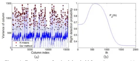
training in this experiment. All images in this paper are acquired from the ANDOR iXon 888 Electron-Multiplying CCD (EMCCD) of the photometric system in Yunnan Astronomical Observatory. Fig.3 (a) shows the Gaussian distribution curves of target and background columns with our method, which has favorable separability with the variance feature. In Fig.4 (a), there are 351 target columns (red points) detected with K-means, but some columns with faint target pixels whose row variances are not so large have not been singled out. Nevertheless, using the optimal threshold achieved by our method, 398 target columns (black points) are detected. That is, the missing columns are almost successfully found back, which is confirmed by artificial examination.

Figure 4. Experiment of optimal threshold for variance vector. (a) Comparison of detection results with K-means and our method; (b) Objective function curve. There are 30 images for training in this experiment. It is shown in (a) that the red points represent the detection results by K-means, while the black points denote the detection results of

In Fig.4 (b), α is taken as 0.5 to avoid the missing of weak targets. It is obvious that the maximum value of the objective function Pd(th) exists, and that the optimal threshold can be easily solved.

Additionally, in order to verify the application range, we add Gaussian noises of different variances ranging from 0.05 to 0.5 with 0.05 interval into these 30 images. All numerical parameters are normalized, which correspond to the operation of adding noises with intensities ranging from 0 to 1. Fig.5 (a) illustrates that the performance of variance vector detection decreases sharply when the variance of the added noise reaches 0.25. Fig.5 (b) shows one of the 30 sample images added with diverse noises. When the noise is stronger than the 4th sub-figure of Fig.5 (b), our method becomes sensitive. Therefore, the better preprocess technique is required to suppress the noise efficiently, such as morphological filtering, wavelet filtering, etc.

TABLEI.

DETECTION TIME IN MATLAB.

Method Opening High-pass Wavelet Our

Detection(s) 0.2895 0.5951 2.3203 0.3180

B. Algorithms Comparison Experiments

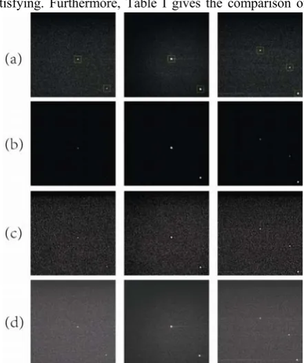
To see the actual effect of our method, we compare our results with those of morphology based, high-pass filtering based and wavelet based algorithms. Due to the limited space, only three groups of visual comparisons are illustrated in Fig.6, from which we can observe that our method is able to detect multiple targets being either small or large. The results of morphological method are shown in Fig.6 (b), and it performs well in Fig.6 (b-1). But you can find that there are many false-alarm points detected around the true targets if enlarging Fig.6 (b-2). It demonstrates that the detection result of opening operation is closely related to the sizes of the target and structuring element. But the space targets actually presenting in images are not always the fixed size. From the results of Fig.6 (c) and (d), the combination of high-pass filtering and local Otsu [18] segmentation cannot exclude the noise points well, while the performance of wavelet detection is

satisfying. Furthermore, Table I gives the comparison of

running time, and all experiments are performed using Matlab 7.11 (R2010b), on a PC with a dual-core 2.20GHz CPU and 2GB RAM Windows 7 machine. In this experiment, our algorithm implements three parts including the preprocessing, detection and location. While the other three algorithms only take the corresponding filtering operations. It indicates that the 2th variance based method has favorable realizability to meet the real-time application, but the wavelet method having favorable detection result is a bit time-consuming. That is, our method has much room for improvement to be applied in the tracking systems of high real-time requirement. At the same time, owning the least running time in these four algorithms, an improved morphological method of adaptive scale being proposed latter may be also applicable in the detection of space targets.

The 2th variance based algorithm is operated in the variance space, and how about the results of similar operations in grayscale space directly. Two universal clustering methods of K-means and adaptive threshold are taken for example, and the same samples of the 30 images mentioned above are adopted for training in this experiment. The process of K-means just likes our method, but the sample elements are 30×512×512 pixels instead here. Meanwhile, the process of adaptive threshold algorithm is described briefly in the caption of Fig.7. After the unsupervised binary classification, the probability density functions of f1(x) and f2(x) for the target and background pixels are also estimated with the Gaussian model. As shown in Fig.7, the result of K-means in grayscale space is undesirable. That is due to the fact that

Figure 5. Detection probabilities with different noises. (a) Detection probability curve; (b) Sample image with noises.Pdetectiondescribed in (9) is

the weighted sum of Ptarget and Pback, and the weight coefficient α is taken

as 0.5. The Guassian noises with various intensities are added into the 30 sample images. (a) shows the curves of the three kinds of detection probabilities mentioned above varying with the noise intensity. The four

sub-figures of (b) are one of the 30 sample images added with different noises, the normalized intensities of which are respectively 0, 0.1, 0.2

and 0.3.

Figure 6. Comparison of different algorithms. (a) Original images and our method; (b) Morphological opening operation; (c) High-pass filtering and local Otsu; (d) Wavelet. In this experiment, three images are selected

to test: the first one with two small targets, the second one with two larger targets than the first one and the third one with three targets whose

the target and background groups are hardly separated well, and the final threshold is too low to exclude the noise points from targets. The adaptive threshold algorithm performs much better than K-means, but it may miss lots of weak points from the distribution map as the calculated threshold is about 116.3. Step back to Fig.4 (a), the variance subspace enlarges the scale and increases the discrimination. Table II gives further on the comparison of running time in Matlab in the same machine mentioned above. Working on the grayscale space augments the calculation amount largely, especially for the large sample analysis. We can see K-means costs so much training time, while our method based on variance subspace is most time-saving. The adaptive threshold, known as a simple method, is also satisfying in the execution time. Nevertheless, the extended operations should be supplied to determinate the better threshold and decrease the leaking-detection, like the reconfirmation mechanism.

TABLEII.

CLUSTERING AND FITTING TIME IN MATLAB.

Method K-means Adaptive threshold Our Method

Clustering(s) 47.847 0.794 0.444

C. Tracking Experiments

Given the detection experiment, let us focus on the target tracking. In this tracking experiment, we take 140 frames of continuous images with the same size of 768×576 for testing, which have one moving space target.

Fig.8 illustrates the sample images of tracking. In the detection algorithm as represented in section III, the research space is the whole image, while it becomes the area of the larger window shown in Fig.8 at the tracking stage. In other words, we operate the method of variance vector detection only in this predicted window, which largely reduces the calculation amount to satisfy the real-time requirement. The size of this larger window in image is 64×64 in this paper. If it is set to be too large, some

disturbance may be brought in. While if it is too small, the target may escape out of this prediction window as a result of the limited prediction precision. Then the location of the target can be easily calculated with the various centroid algorithms, and the smaller window in Fig.8

whose size values 40×40 is the final detection result for

each frame.

In our tracking algorithm, the parameter β denoting the learning rate should be properly ensured. To search the optimal β , we define two indicator functions as follows:

] ) [(

2 1 ] ) [(

2

1 2 2

c c r

r X E Z X

Z E

RMSE= − + − , (15)

) (

2 1 ) (

2 1

c c r

r X D Z X

Z D

SDE= − + − , (16)

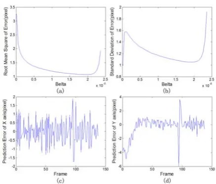
Figure 9. Prediction errors. (a) RMSE respecting β; (b) SDE respecting β; (c) Prediction error of X axis with _β=2.0×10−6_{; (d)}

Prediction error of Y axis with _β=2.0×10−6_{. There are 140 768×576}

images to test the tracking algorithm, and β is the learning rate appearing in the section III.C.

Figure 8. Tacking samples. (a) The 4th frame; (b) The 16th frame; (c) The 32th frame; (d) The 64th frame; (d) The 94th frame; (d) The 128th frame. The lager windows (yellow) in figures are prediction areas with our tracking algorithm, while the smaller ones (red) are the detection

results with our detection method. Figure 7. Distribution diagrams of grayscale space based algorithms. (a)

K-means; (b) Adaptive threshold. The samples are still the 30 images mentioned in section IV.A. f1(x)and f2(x) are the fitting curves for the

target and background pixels in grayscale space, as shown in (a) and (b). The threshold achieved with the algorithm of K-means is 23.2, while the threshold obtained with the method of adaptive threshold is 116.3. The adaptive threshold employed in this paper is briefly described as follows: 1. Initialize the threshold; 2. Calculate the centres of the two classes, and

where Zr and Xr are respectively the measured value and prediction value in the X axis (row direction), meanwhile, Zc and Xc are respectively the measured value and prediction value in the Y axis (column direction). The symbol E indicates the mean evaluation, and D denotes the variance evaluation. Fig.9 (a) and (b) show the values of (15) and (16) varying the different β, from which the optimal β should be 2.0×10-6 around.

Experiments demonstrate that the tracking errors in these 140 frame images oscillate viciously if β deviates from its optimum value a lot. Therefore, β is taken as 2.0×10-6

in this experiment, and the corresponding tracking errors in X and Y axises are shown in Fig.9 (c) and (d). Note that the speed of this selected space target is about 0.5 degree per second, and the frame frequency is 25 frames per second. From the curves, the precision of tracking is about one pixel once the model parameters θ have stabilized after multiple iterations. The tracking error becomes larger when the movement of target changes suddenly, but it can gradually turn to the normal level in several iterations. At last, we test the running time in Matlab within the same operating environment above. The whole running time for the 140 images is 3.1619s, and the average processing time of each frame is about 22.6ms. Thus, our method can be applicable to the high frame rate CCD for space target detection and tracking.

V. CONCLUSIONS

The 2th variance feature based method supplies a novel idea for the problem of space target detection and tracking. Through learning from the training samples, we propose the fusion algorithm of K-means learning and WMRP criterion to determine the optimal threshold in variance vector detection, and the multi-scale threshold algorithm to secondarily extract the true targets in 2th variance detection. We project the grayscale space into the variance subspace of two-dimension, which not only reduces the execution time but also ensures the detection performance. The tracking algorithm based on the Markov theory gives a simple but effective dynamic model which largely saves the detection time for each frame. Furthermore, we can adopt other features together with the 2th variance to raise the reliability of algorithm, and segment the image into four blocks or more to decrease the sensitivity of variance vector detection for the noised background. In addition, the better de-noising technique can be jointed with our method to suppress the background. Experiments demonstrate that the variance detection algorithm of two-step framework can effectively and rapidly detect multiple space targets, and the cooperative working of the detector and tracker can competent the conventional satellite tracking task of high real-time demand.

ACKNOWLEDGMENT

This work was supported in part by the National Natural Science Foundation (NSFC) of China under

Grant No.10978025. The authors gratefully acknowledge the constructive comments from the reviewers, which significantly improve the representation and quality of this manuscript.

REFERENCES

[1] Myrtille Laas-Bourez, David Coward, Alain Klotz and Michel Boer, “A robotic telescope network for space debris identification and tracking,” Advances in Space Research, vol. 47, pp. 402-410, Feb. 2011.

[2] Blostein S D and Huang T S, “Detection of small moving objects in image sequences using multistage hypothesis testing,” IEEE Proc. on ICASSP., New York, pp. 1068-1071, Apr. 1988.

[3] L. A. Johnston and Krishnamurthy V, “Performance analysis of a dynamic programming track before detect algorithm,” IEEE Aerospace and Electronic Systems, vol. 38, pp. 228-242, Jan. 2002.

[4] Tonissen S M and Evans R J, “Peformance of dynamic programming techniques for Track-Before-Detect,” IEEE Aerospace and Electronic Systems, vol. 32, pp. 1440-1451, Apr. 1996.

[5] Punithakumar K, Kirubarajan T and Sinha A, “A sequential monte-carlo Probability hypothesis density algorithm for multi-target track-before-detect,” SPIE Proc. SDPST., California, pp. 59131S1, Sept. 2005.

[6] Alexander Tartakovsky, “Effective adaptive spatial-temporal technique for clutter rejection in IRST,” SPIE Proc. SDPST., Orlando, pp. 85-95, July 2000.

[7] He Deng, Jianguo Liu and Zhong Chen, “Infrared small target detection based on modified local entropy and EMD,” Chinese Optics Letter, vol. 8, pp. 24-28, Jan. 2010. [8] Dong Hongyan, Li Jicheng and Shen Zhenkang, “Small

target detection based on high-pass filtering and order filtering,” System Engineering and Electronics, vol. 26, pp. 596-598, May 2004.

[9] Jean-Francois Rivest and Roger Fortin, “Detection of dim targets in digital infrared imagery by morphological image processing,” Optical Engineering, vol. 35, pp. 1886-1893, July 1996.

[10]Deng Ze-Feng, Yin Zhou-Ping and Xiong You-Lun, “High probability impulse noise-removing algorithm based on mathematical morphology,” IEEE Signal Processing Letter, vol.14, pp. 31-34, Jan. 2007.

[11]Giuseppe B, Angelo C and Antonio P, “Small Target Detection Using Wavelets,” IEEE Proc. on Pattern Recognition, Brisbane, pp. 1776-1778, Aug. 1998.

[12]Damerval, Christophe, Meignen and Sylvain, “Blob detection with wavelet maxima lines,” IEEE Signal Processing Letter, Vol. 14, pp. 39-42, Jan. 2007.

[13]Barbara F, La Scala and Robert R. Bitmead, “Design of an extended kalman filter frequency tracker,” IEEE Signal Processing, Vol. 44, pp. 739-742, Mar. 1996.

[14]Eric A. Wan and Rudolph van der Merwe, “The unscented Kalman filter for nonlinear estimation,” IEEE Proc. on ASSPCC., Lake Louise, pp. 153-158, Oct. 2000.

[15]Magnus Norgaard, Niels K. Poulsen, Ole Ravn, “New developments in state estimation for nonlinear systems,” Automatica, Vol. 32, pp. 1627-1638, Nov. 2000.

[16]Filip Hroch, “The robust detection of stars on CCD images,” Experimental Astronomy, vol. 9, pp. 251-259, 1999.

[18]Nobuyuki Otsu, “A Threshold Selection Method from Gray-Level Histograms,” IEEE Systems, Man and Cybernetics, vol. 9, pp. 62-66, Jan. 1979.

Tao Huang received Bachelor degree in Physics (optics) from China University of Geosciences, China. He is currently a PhD student in the Photoelectric tracking and control engineering at Yunnan Astronomical Observatory, Chinese Academy of Sciences, China. His research interests include detection and tracking of small target, machine learning and automation technique.

Yaoheng Xiong received PhD degree in astrometry and celestial mechanics from Yunnan Astronomical Observatory, Chinese Academy of Sciences, China. He is currently a professor in the astronomical technique at Yunnan Astronomical Observatory. His research interests include

detection and location of space target, adaptive optics and lunar laser ranging.

Zhulian Li received PhD degree in astrometry and celestial mechanics from Yunnan Astronomical Observatory, Chinese Academy of Sciences, China. She is currently a senior engineer in the automation technique at Yunnan Astronomical Observatory. Her research interests include detection of space target and satellite laser ranging.

Yu Zhou received PhD degree in astrometry and celestial mechanics from Yunnan Astronomical Observatory, Chinese Academy of Sciences, China. She is currently a associate professor in the optical technique at Yunnan Astronomical Observatory. Her research interests include photometric measurement and high energy laser.