BFGS-GSO for Global Optimization Problems

(1)

BFGS-GSO for Global Optimization Problems

Aijia Ouyang1,2

1. College of Computer, Hunan Science & Technology Economy Trade Vocation College, Hengyang, China Email: [email protected]

2. College of Information Science and Engineering, Hunan University, Changsha, 410082, China

Libin Liu*

Department of Mathematics and Computer Science, University of Chizhou, Chizhou, 247000, China Email: [email protected]

Guangxue Yue

College of Mathematics and Information Engineering, Jiaxing University, Jiaxing, 314001, China

Email: [email protected]

Xu Zhou and Kenli Li

College of Information Science and Engineering, Hunan University, Changsha, 410082, China Email: {xuzhou, lkl}@hnu.edu.cn

Abstract—To make glowworm swarm optimization (GSO) algorithm solve multi-extremum global optimization more effectively, taking into consideration the disadvantages and some unique advantages of GSO, the paper proposes a hybrid algorithm of Broyden–Fletcher–Goldfarb– Shanno (BFGS) algorithm and GSO, i.e., BFGS-GSO by adding BFGS local optimization operator in it, which can solve the problems effectively such as unsatisfying solving precision, and slow convergence speed in the later period. Through the simulation of eight standard test functions, the effectiveness of the algorithm is tested and improved. It proves that the improved BFGS-GSO abounds in better multi-extremum global optimization in comparison with the basic GSO.

Index Terms—Global optimization; GSO; BFGS operator; BFGS-GSO; function

I. INTRODUCTION

The global optimization problems on nonlinear function of continuous variable widely exist in the industrial and agricultural production and scientific experiments, the global optimization method of the functions plays an important role for solving many practical problems and developing many edge disciplines. The traditional global optimization methods are mostly based on the gradient method, the convergence of these methods often depends on the selection of initial points, and the computing process usually terminates the local optimum.

In literature [1], S. Gao et al. propose a hybrid algorithm, which combine ant colony algorithm with genetic algorithm, to solve the global optimization problem. In 2012, T. Chen et al. propose artificial tribe

algorithm to solve the functions optimization problem [2]. To solve the multimodal function problem, D. shen et al. [3] propose a crowding differential evolution algorithm. In [4], an improved particle swarm optimization algorithm is proposed to find the global optimum solutions with adaptive genetic strategy. In [5], an invasive weed optimization algorithm is proposed to solve the high-dimensional function optimization problem. The above algorithms are intelligence algorithms, these methods have excellent global search ability but the computing precision is not high. Y. Cheng et al. propose a quasi-Newton method for function minimization [6]. In [7] and [8], to solve the global optimization problem, the simplex method and the Powell’s method are proposed. For global optimization, a metropolis algorithm, which combined with Hooke-Jeeves local search method, is proposed [9]. In [10], R. Chelouah and P. Siarry combine the Nelder-Mead algorithm with genetic algorithm to solve the continuous minimal functions optimization problem. The above algorithms are mathematical methods, they have nice local search ability but they have weak robustness global search ability.

As a global and local optimization techniquee newly proposed in swarm intelligence, glowworm swarm optimization (GSO) algorithm with speedy searching of extreme range and high efficiency [11]is mainly used to solve the problems of multi-extremum global and local optimization. In view of its good and stable multi-extremum optimization, GSO has excellent performance in sound source localization [12], multi-odor source localization [13], multiple mobile information source tracking [14] and mobile robot system [15]and is widely applied in numerical optimization [16-17] and combinatorial optimization [18-19]. Nevertheless, there are still weaknesses in that the local solving precision and later convergence rate don’t work as well as some classic This work is supported by the NSFC (No.11301044).

(2)

local searching algorithm [20-24]. Furthermore, its population size shows exponential growth with the increase of searching areas and dimensions, which leads to long computing time and limited performance in optimization.The later oscillation phenomenon also has some effects on the solving precision of the algorithm.

In this paper, we propose a hybrid algorithm, termed BFGS-GSO algorithm. We use GSO algorithm to perform a global search and we use BFGS algorithm for performing a local search. The GSO algorithm can converge quickly and the BFGS algorithm can compute precisely in the BFGS-GSO algorithm. We realize the program of BFGS-GSO algorithm for the first time and the performance of proposed algorithm is tested by the Benchmark functions. The experimental results show that it is a competitive algorithm.

The rest of this paper is organized as follows: we describe the principle of basic GSO and BFGS algorithm in Section II; then we propose the algorithm of BFGS-GSO, in Section III, we present the algorithm steps and flowchart; we perform the simulation experiments and discuss the experimental results in Section IV; at last, we conclude the paper in Section V.

II.PRINCIPLE OF THE ALGORITHM AND BACKGROUND

A. Basic GSO Algorithm

Imitating glowworm’s flying, aggregation, courtship, feeding and other natural activity, the basic GSO algorithmis a swarm intelligent bionic algorithm where a group of randomly distributed points in the searching space represent the glowworm swarm, and the proportional value proportionate to the fitness value of point represents the luciferase value glowworms carry. The glowworm swarm move as one with the help of luciferin. The greater the luciferase value the individual glowworm carries and more light it emits, the more attractive it is to its companions [25-28].

However, each individual glowworm only attracts companions in decision domain, also called the neighbourhood, the radius value of which is represented by rd. Only when glowworm j is within this range and its

luciferase value is higher than glowwormi, is it likely to

become glowworm i’s neighbour and its moving objects. Besides, the decision domain size is limited in the visual range of glowworms (that is 0<rd<rs, rs represents visual

radius of glowworms). GSO algorithm consists of two stages, luciferin renewal and glowworm moving [29-31]. 1)Luciferin renewal stage: At the beginning and the end of each iteration, the algorithm uses Formula 1 to update luciferin value of each glowworm, so that glowworm luciferin value will vary with the fitness value and attenuate with the increase of algorithm iteration. Formula 1 is as follows.

l t

_i

( ) (1

= −

ρ

) (

l t

_i

− +

1)

γ

J x t

( ( ))

_i (1) In the above formula,ρ∈(0,1) represents the luciferin attenuation factor,γ represents the fitness values of the proportionality constant, and l ti( ) represents at the moment of

t

the luciferin value of glowwormi.

2)Glowworm moving stage: After the phthalein resorcinol is renewed, the algorithm reaches the glowworm moving stage when each glowworm uses the roulette selection to select a neighbor glowworm as its moving object. Use Formula 2 to calculate the probability of each neighbour’s being selected, and use formula 3 to calculate the target position after the glowworm’s moving. At the end of the stage, use formula 4 to renew decision domain radius of each glowworm.

The selection probability formula is as follows,

( )

i j i ij k i

k N t

l t

p t

l t

∈

−

=

−

∑

(2)

In the formula above,p tij( )represents at the moment of

t the likelihood of glowworm i moving to glowworm j,

and N ti( ) represents at the moment of t the number of neighbours glowworm i has.

The target position calculation formula is as follows,

( )

(

1)

( )

*

( )

j i

i i

j i

x t

s

x t

⎛

₋

⎞

+ =

+

⎜

_⎜

⎟

_⎟

−

⎝

⎠

(3)

In the formula above,x ti( )（ ( )

m i

x t ∈R ） represents at

the moment of t the location of glowworm i ,and || ||•

represents the Euclid standard operator, and s( 0)> represents the moving step of glowworm i.

Neighbourhood radius updating formula is as follows,

(

1) min{ ,max{0, ( )

(

( ) )}}

i i

d s d t i

r t

+ =

r

r t

+

β

n

−

N t

(4)

In the above formula, i( )

d

r t represents at the moment of

t the decision domain radius of glowworm i , β

represents at the moment of t the neighbour set of

glowworm i, and nt represents the maximum number of

neighbour glowworms.

B. BFGS Theory

Proposed by Broyden, Fletcher, Goldfarb and Shanno, et al in 1970, BFGS methodis a quasi-Newton method, characteristic of two terminations, global and super-linear convergence, and the searching direction generated by the algorithm is conjugate. BFGS method is an efficient local algorithm, and the main steps to solve the minimum are as follows,

Step 1 Determine the variable dimensionnand BFGS method convergence precisionε≥0, and take the initial point 1 n

X ∈R ;

Step 2 Compute g1= ∇f X( 1) . If g1 ≤ε , make

* 1

X =X ，andf*= f X( 1)，and the calculation stops; if

not, turn to Step3;

Step 3 Make k=1,H₁=I_n;

Step 4 Make k

k k

(3)

Step 5

0

min ( k k) ( k k)

k _λ f X Z f X Z

λ：_≥ +λ = +λ , make

1

k k k

X + =X +λZ ;

Step 6 Compute 1 ( 1) k k

g ₊ = ∇f X + ,if gk+1 ≤ε , make

* k 1

X =X + , * ( k 1)

f = f X + , and the calculation stops; if not, turn to Step7;

Step 7 Make k 1 k k

X X + X

Δ = − Δ =gk gk+1−gk, compute

1 (1 )

-T T

k k k k k

k k T

k k k k

g H g X X

H H U

X g X g

+ = + +Δ Δ Δ Δ

Δ Δ Δ Δ ,

k Tk k k k Tk T

k k

X g H H g X

U

X g

Δ Δ + Δ Δ

=

Δ Δ ;

Step 8 Make k= +k 1, turn to Step 4.

III.BFGS-GSOALGORITHM DESCRIPTION

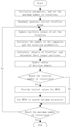
A. BFGS-GSO Algorithm’s Specific Implementing Steps Step 1 Initialize the parameters ρ,γ,β,nt,s,l0in GSO algorithm, and set the maximum iteration numbers

max

T of BFGS-GSO algorithm;

Step 2 Renew the l

uciferin value

of every individual of the glowworm swarm by using Formula 1;

Step 3 Calculate glowworm the peers ofi (any

individual in the swarm) within the decision domain and the probability that every glowworm can be chosen as the target by using Formula 2;

Step 4 Determine glowworm i's alternative j(j∈Ni(t)) by using roulette rule, and renew the target

position of the glowworm by using Formula 3;

Start

Randomly generate initial fireflies group

Update luciferin values of all the fireflies

Calculate the number of the companion and the selection probability

Calculate objects of fireflies and determine their target positions

Update radius of decision domain

Provide initial values for BFGS

Use BFGS to search optimum accurately

End

Reach the interval number of iterations?

Yes

Yes No

No

Reach the maximum number of iterations?

Initialize parameters, and set the maximum number of iterations

(4)

Step 5 Renew the decision domain radius of glowworm i by using Formula 4;

Step 6 Turn to Step 7 if interval iteration number is reached; otherwise, turn to Step 9;

Step 7 Determine the optimal individual ibest in the

swarm and its peer number nbest in sight, and construct

the initial BFGS of BFGS operator by using ibest and its

peers in sight.

Step 8 Locally optimize the optimal decision region by using BFGS operator;

Step 9 Record the result and exit the iteration if presupposed maximum iteration number is reached; otherwise, turn to Step 2 and continue the iteration.

B. Flowchart of BFGS-GSO Algorithm

The flowchart of BFGS-GSO is as in Figure 1.

IV.EXPERIMENTAL RESULTSA.TEST FUNCTIONS OF THE EXPERIMENT

A. Benchmark Functions

The eight standard test functions, which are multi-peak, morbid and not declined to achieve ideal optimizing result when using traditional optimizing method, are used to compare the algorithm discussed in this paper with the basic GSO algorithm. The three-dimension images of the four test functions are as follows, the eight standard test functions are the typical global optimization functions, they have an excellent ability to verify the whole performance of each algorithm.

2 2

1 2 2 2

sin(

0.5)

0.5 [1.0 0.001(

)]

x

y

f

x

y

+

−

=

−

+

,

[ 4,4];

[ 4,4]

x

∈ −

y

∈ −

;

2 2 0.25 2 2 0.1 2

2

(

)

[sin(50 (

) )

1.0]

f

=

x

+

y

×

x

+

y

+

,

[ 100,100]

x

∈ −

;

y

∈ −

[ 100,100]

; 2

3

13 ((5

)

2)

)

f

= − + +

x

− × − ×

y

2

29 x

((

y

1)

y

14)

y

)

− + +

+ × −

×

[ 10,10],

[ 10,10]

x

∈ −

y

∈ −

;

2 2

4

1

1 (

) cos( ) cos(

)

4000

2 y

f

= +

x

+

y

−

x

×

,

[ 10,10]

x

∈ −

;

y

∈ −

[ 10,10]

;

2 5

1

,( 30)

n

i i

f x n

=

∑

=

（x） ;

1

2 2 2

6 1

1

( ) n (100( _i _i) (1 _i) ),( 30) i

f x x x x n

−

+ =

=

∑

− + − = ;

2 7

1 1

1

( ) cos( ) 1,( 30) 4000

n n i i

i i

x

f x x n

i

= =

=

∑

−

∏

+ = ;

2 8

1

( ) n ( _i 10cos(2 _i) 10),( 30)

i

f x x πx n

=

∑

− + = ;

B. Parameter Setting

As is displayed in Table 1, the fixed parameter value of BFGS-GSO and GSO algorithm derives from documents so as to guarantee the authenticity and effectiveness of the experiment. Meanwhile, population sizes of the two algorithms are both 100 to make an accurate comparison. In addition, glowworm viewing ranges and moving step lengths of the two vary in accordance with different target functions so that the two algorithms achieve the best optimizing effect according to different target functions. As to f1, f2, f3and f4, the glowworm viewing range radius values of the two are 1.5, 30, 5 and 5 respectively, and the moving step lengths are 0.03, 0.3, 0.03, and 0.03 respectively.

TABLE I.

PARAMETER SETTING OF BFGS-GSO AND GSO ALGORITHM

ρ γ β nt l0 δ γ η

0.4 0.6 0.08 5 5 1.0 2.0 0.5

Figure 2. Three-dimensional images of f1

(5)

Figure 6. Convergence comparison of f1

C. Test Platform

Windows XP combined with MatLab2012a is served as the simulation software platform, while Intel® Celeron® CPU 3.06Hz 3.07GHz and PC with memory 4.00GB work as the simulation hardware platform.

D. Result Analysis of the Simulation

(6)

under fixed precision value

ε

of the experimental result, the second is one which compares solving precisions when the maximum iteration number is fixed. Every standard test function undergoes 100 independent tests in order to eliminate the initial value's effect on the result of the experiment.

As is exhibited in Table 2, the convergence effect of BFGS-GSO algorithm is preferable than GSO. Within the

presupposed maximum iteration number, BFGS-GSO enjoys better solving precision judging from Table 3. BFGS-GSO achieves theoretially optimum value in terms of f1 and f8 shown from both tables. Convergence curves

of Figure 6 and Figure 13 manifest that BFGS-GSO enjoys better convergence rate and solving precision in comparison with GSO.

TABLE II.

CONVERGENCE RATE OF CONTRAST ON TWO METHODS

Precision Methods Min-IT Max-IT Mean-IT Optimal _times Convergence _rate

f1 (ε=10-7) _{BFGS-GSO 76 114}GSO 116 195 165 ₉₁ 0 ₁ 15% _95%

f 2 (ε=10-4) _{BFGS-GSO 140 158}GSO 271 280 276 ₁₅₃ 0 ₀ _90%3%

f 3 (ε=10-5) _{BFGS-GSO 102 124}GSO 187 198 192 ₁₁₇ 0 ₀ _92%6%

f 4 (ε=10-7) _{BFGS-GSO 25 99}GSO 101 198 160 ₇₆ ₁₄0 _100%41%

f5 (ε=10-3) _{BFGS-GSO 56 79}GSO 0 0 0 ₆₄ 0 ₀ _96%1%

f 6 (ε=10-1) _{BFGS-GSO 36 81}GSO 0 0 0 ₆₂ 0 ₀ _99%2%

f 7 (ε=10-5) _{BFGS-GSO 42 70}GSO 158 191 175 ₅₉ 0 ₀ _98%2%

f 8 (ε=10-1) _{BFGS-GSO 39 117}GSO 0 0 0 ₉₇ 0 ₀ _99%3%

TABLE III.

COMPUTING VALUES OF CONTRAST ON TWO METHODS

Function Method Best value Worst value Mean value

f 1 BFGS-GSO 1 9.902840901219776e-01_{GSO 9.702840901016672e-01} _{8.902794766551073e-01} 9.999840901224632e-01 _{9.272348710046113e-01}

f 2 BFGS-GSO 1.055902964335211e-13_{GSO 1.809828012643451e-03} 2.214176085496879e-06_{3.469580568556631e-02} 6.459276747376119e-10 _{1.487490229867432e-01}

f 3 BFGS-GSO 1.928969612645085e-09_{GSO 1.017462621198369e-06} 1.219861367861428e-06_{2.910471332073746e-01} 1.830965737445319e-07 _{9.416975050855370e-01}

f 4

BFGS-GSO 0 3.086190795142940e-07 3.227826894658392e-10 GSO 6.589637380205460e-08 6.446040057284108e-01 4.148428437433793e-03

f 5

BFGS-GSO 2.500343939721753e-08 3.547220632776181e-03 7.344282622010108e-04 GSO 3.726577273473546e-04 1.083645821191223e-01 9.563874302131754e-02

f 6

BFGS-GSO 2.554490914899631e-05 3.486928796398612e-01 8.454674180661280e-02 GSO 8.611721663699928e-01 7.444845039640595e+02 5.621410451607271e+01

f 7

BFGS-GSO 3.581225872184055e-08 1.534199177949786e-04 1.620721642303850e-06 GSO 2.671315883217245e-05 4.578660307778230e+01 6.466177666261162e-00

f 8

BFGS-GSO 8.350803389374136e-05 8.650279035353914e-02 7.597490110230252e-01 GSO 6.674463238927735e-01 4.479180635155838e+02 5.404773469221640e+01

V.CONCLUSION

To make GSO solve multi-extreme global optimization more effectively, given that GSO carries the advantages such as speedy searching of extreme range, high efficiency and not being apt to fall into local extremum and the disadvantage of slow convergence rate in the later period, the paper puts forward BFGS glowworm swarm mixed optimization algorithm, which makes the most of the global extreme value searching ability of GSO and local precision-pursuing ability of BFGS. By carrying out BFGS local optimization among optimal individual in the swarm and its peers in sight every regular algebra, BFGS-

GSO promotes the convergence rate and the solving precision substantially. In conclusion, BFGS-GSO is feasible and effective in terms of solving multi-extremum global optimization.

ACKNOWLEDGMENT

(7)

Ministry of Education of China (Grant No.20100161110019), the Program for New Century Excellent Talents in University (Grant No.NCET-08-0177), the Research Foundation of Education Bureau of Hunan Province, China(Grant No.13C333), the Natural Science Foundation of Zhejiang, China (No.LY12F02019), the public technology application research of Zhejiang, China(No.2011C23130), the Jiaxing Committee of Science and Technology, China(No.2012AY1027).

REFERENCES

[1] S. Gao, Z. Zhang, and Cungen Cao. “A Novel Ant Colony Genetic Hybrid Algorithm,” Journal of Software, vol.5,

no.11, pp.1179-1186, 2010.

[2] T. Chen, Y. Wang, and J. Li, “Artificial Tribe Algorithm and Its Performance Analysis,” Journal of Software, vol.7,

no.3, pp.651-656, 2012.

[3] D. Shen, and Y. Li, “Multimodal Optimization using Crowding Differential Evolution with Spatially Neighbors Best Search,” Journal of Software, vol.8, no.4, pp.932-938,

2013.

[4] Y. Cheng, Y. Ren, and F. Tu, “An Improved Particle Swarm Optimization Algorithm based on Adaptive Genetic Strategy for Global Numerical Optimal,” Journal of

Software, vol.8, no.6, pp.1384-1389, 2013.

[5] L. Xie, A. Ouyang, L. Liu, M. He, X. Peng and X. Zhou, “Chaotic Hybrid Invasive Weed Optimization for Machinery Optimizing,” Journal of Computers, vol.8, no.8,

pp.2093-2100, 2013.

[6] D. F. Shanno, “Conditioning of quasi-Newton methods for function minimization,” Mathematics of computation,

vol.24 no.111, pp.647-656, 1970.

[7] M. Sniedovich E. Macalalag, and S. Findlay, “The simplex method as a global optimizer: A c-programming perspective,” Journal of Global Optimization, vol.4, no.1,

pp.89-109, 1994.

[8] O. Kramer, “Iterated local search with Powell’s method: a memetic algorithm for continuous global optimization,” Memetic Computing, vol.2, no.1, pp.69-83,

2010.

[9] A. C. Rios-Coelho, W. F. Sacco, and N. Henderson, “A Metropolis algorithm combined with Hooke–Jeeves local search method applied to global optimization,” Applied

Mathematics and Computation, vol.217, no.2, pp.843-853,

2010.

[10]R. Chelouah, and P. Siarry, “Genetic and Nelder–Mead algorithms hybridized for a more accurate global optimization of continuous multiminima functions,” European Journal of Operational

Research, vol.148, no.2, pp.335-348, 2003.

[11]K. N. Krishnanand, D. Ghose, “Glowworm swarm optimisation: a new method for optimising multi-modal functions,” International Journal of Computational

Intelligence Studies, vol.1, no.1, pp.93-119, 2009.

[12]K. N. Krishnanand, D. Ghose, “Theoretical foundations for multiple rendezvous of glowworm-inspired mobile agents with variable local-decision domains,” American Control

Conference, USA, June 2006, pp. 3588-3593.

[13]P. Amruth, K.N. Krishnanand, D. Ghose, “Glowworms-inspired multirobot system for multiple source localization tasks,” Workshop on Multi-robot Systems for Societal Applications, International Joint Conference on Artificial

Intelligence, India, January 2007, pp.32-7.

[14]K. N. Krishnanand, D. Ghose, “Chasing multiple mobile signal sources: A glowworm swarm optimization approach,” Third Indian International Conference on

Artificial Intelligence, India, December, 2007,

pp.1308-1327.

[15]K. N. Krishnanand, D. Ghose, “Detection of multiple source locations using a glowworm metaphor with applications to collective robotics,” IEEE Swarm

Intelligence Symposium, USA, June 2005, pp. 84-91.

[16]Y. YANG, Y. ZHOU, Q. GONG, “Hybrid Artificial Glowworm Swarm Optimization Algorithm for Solving System of Nonlinear Equations,” Journal of

Computational Information Systems, vol.6, no.10, pp.

3431-3438, 2010.

[17]Y. Yang, Y. Zhou, “Glowworm Swarm Optimization Algorithm for Solving Numerical Integral,”

Communications in Computer and Information Science,

vol.134, pp.389-394, 2011.

[18]Q. Gong, Y. Zhou, Y. Yang, “Artificial Glowworm Swarm Optimization Algorithm for Solving 0-1 Knapsack Problem,” Advanced Materials Research, Vol.143-144,

pp.166-171, 2011.

[19]J. Nelder, R. Mead, “A simplex method for function minimization,” Computer Journal, Vol.7, pp.308-313,

1965．

[20]K. E. Parsopoulos, M. N. Vrahatis, “Initializing the particle swarm optimizer using the nonlinear simplex method,”

Advances in Intelligent Systems Fuzzy Systems,

Evolutionary Computation, USA:WSEAS Press,

pp.216-221, 2002.

[21]J. Kenedy, R. Ebedum, Swarm Intelligence, Morgan: Kanfmann Publishers, 2001.

[22]A. M. Nezhad, R. A. Shandiz, A. E. Jahromi, “A particle swarm–BFGS algorithm for nonlinear programming problems,” Computers & Operations Research, Vol.40, no.4, pp.963-972, 2013.

[23]M. S. Bazaraa, H. D. Sherali, L. M. Shetty, Nonlinear

programming: theory and algorithms, New York: John

Wiley and Sons; 2006.

[24]J. Nocedal, S. J. Wright, Numerical optimization. Springer,

2006.

[25]K.N. Krishnanand, D. Ghose, “Theoretical foundations for rendezvous of glowworm-inspired agent swarms at multiple locations,” Robotics and Autonomous Systems,

Vol.56, no.7, pp.549-569, 2008.

[26]K. N. Krishnanand, D. Ghose, “Glowworm swarm optimization for simultaneous capture of multiple local optima of multimodal functions,” Swarm Intelligence,

vol.3, no.2, pp.87-124, 2009.

[27]W.-H. Liao, Y. Kao, Y.-S. Li, “A sensor deployment approach using glowworm swarm optimization algorithm in wireless sensor networks,” Expert Systems with

Applications, vol.38, no.10, pp.12180-12188, 2011.

[28]Q. Gong, Y. Zhou, Q. Luo, “Hybrid Artificial Glowworm Swarm Optimization Algorithm for Solving Multi-dimensional Knapsack Problem,” Procedia Engineering,

vol.15, pp.2880-2884, 2011.

[29]S. Mannar, S. N. Omkar, “Space suit puncture repair using a wireless sensor network of micro-robots optimized by Glowworm Swarm Optimization,” Journal of Micro-Nano

Mechatronics, vol.6, no.3-4, pp.47-58, 2011.

[30]B. Wu, C. Qian, W. Ni, S. Fan, “The improvement of glowworm swarm optimization for continuous optimization problems,” Expert Systems with Applications,

vol.39, no.7, pp.6335-6342, 2012.

(8)

Aijia Ouyang is a Lecturer in the department of computer science and technology, Hunan Science and Technology Economy Trade Vocation College, Hengyang, Hunan province, China. He received the M.E. degree in computer science and technology from Guangxi University for Nationalities, Nanning, China, in 2010. He is currently a Ph.D. candidate of Hunan University, Changsha, China. His research interests include parallel computing, cloud computing, supercomputing, mobile computing, and artificial intelligence. He has published research articles in international conference and journals of parallel computing.

Libin liu is a Lecturer in the Department of Mathematics and Computer Science and Technology at Chizhou University, Chizhou, Anhui Province, China. He received the M.E. degree in computer science and technology from Guangxi University for Nationalities, Nanning, China, in 2009. He is currently a Ph.D. candidate in the College of Mathematics and Computer Science and Technology at South China Normal University, Guangzhou, China. His research interests include parallel computing, and Numerical Methods for Differential Equations. He has published research articles in international conference and journals of Differential Equations.

Guangxue Yue is a Professor in the Department of Computer Science and Technology at Jiaxing University, Jiaxing, China. He received the M.E. degree, the Ph.D. degree in the Department of Computer Science and Technology from Hunan University, Changsha, China, in 2006 and 2012, respectively. His research interests include computer network, distributed system, QoS of streaming media. He has published more than 70 international journals/conference papers on computer network, distributed system and information security.

Xu Zhou is a Lecturer in the Department of Computer Science and Technology at Jiaxing University, Jiaxing, Zhejiang Province, China. She received the B.E. degree in the Department of Computer Science and Technology from Hunan University, Changsha, China, in 2006, and the M.E. degree in the Department of Computer Science and Technology from Hunan University, in 2009, respectively. She is currently a Ph.D. candidate in the College of Information Science and Engineering at Hunan University, Changsha, China. Her research interests include parallel computing, cloud computing, DNA computing and database query. She has published research articles in international conference and journals of supercomputing and DNA computing.