The PID Controller Based on the Artificial Neural Network and the Differential Evolution Algorithm

The PID Controller Based on the Artificial Neural

Network and the Differential Evolution

Algorithm

Wei Lu

The Control Science and Engineering Department of Dalian University of Technology, Dalian, China Email: [email protected]

Jianhua Yang and Xiaodong Liu

The Control Science and Engineering Department of Dalian University of Technology, Dalian, China Email: {jianhuay,xdliu}@dlut.edu.cn

Abstract—The conventional PID

(proportional-integral-derivative) controller is widely applied to industrial automation and process control field because its structure is sample and its robust is well, but it do not work well for nonlinear system, delayed linear system and time-varying system. This paper provides a new style of PID controller that is based on artificial neural network and evolutionary algorithm according to the conventional one’s mathematical formula. The artificial neural network (ANN) is used to approach PID formula and the differential evolution algorithm (DEA) is used to search weight of the artificial neural network. This new controller is proven better control effect in the simulation test. This new controller has more advantages than the conventional one, such as less calculated load, faster global convergence speed, better robust, more independence and adaptability on the plant and independent of human intervention and expert experiences etc.

Index Terms—the artificial neural network, the differential

evolution algorithm, PID controller

I. INTRODUCTION

The conventional PID (proportional-integral-derivative) controller is widely applied to industrial automation and process control, for its control mode is direct, simple and robust. But, there are some disadvantages of PID control. Firstly, it is difficult to regulate the three parameters of PID controller: KP, KI and KD in some control systems. Secondly, the conventional PID controllers generally do not work well for nonlinear system, time-delayed linear system, complex and vague system, time varying systems [1][2][3][4]. Various types of modified PID controller have been developed, such as self-turning PID controller, to overcome the one problem of the regulation conventional PID controller parameter. The fuzzy PID controllers and the neural network PID controllers are also designed for this purpose.

The natural representation of control knowledge make fuzzy controller easy to be understood [13]. But the most fuzzy controllers use two inputs, error, the change rate of

error to approximately behaves like a PD controller, and obviously there would exist steady-state error when industrial process systems are controlled by fuzzy controller. It can eliminate the steady-state error of the control system to consider the integration of error in input of the fuzzy controller. Of course this can be realized by designing ,a fuzzy controller with three inputs, error, the change rate of error and integration of error. However, it will be hard to implement in practice because of the difficulty in constructing control rules base. First, it is not the practice for expert to observe the integration of error. Second, adding one input variable in fuzzy controller will greatly increase the number of control rules [7][8].

The artificial neural network has the ability of learning and function approximation. In addition, the artificial neural network learning processes are independent of human intervention and expert experiences. For such situations, many studies use ANN to approximate PID formula to realize ANN-PID controller. But the learning method of ANN usually adopts some traditional algorithm, including the delta rule, the steepest descent methods, Boltzman’s algorithm, the back-propagation learning algorithm, the standard version of genetic algorithm [9][10][11], etc. These traditional learning methods of ANN exists some deficiency including such as the problem of the slow speed of convergence, local minima, and the large amount of computation of network, etc, which lead to ANN-PID controller is difficult to use actually[15][16]. In this paper, a new ANN PID controller which is based on the differential evolution algorithm (DEA) is proposed. Here, artificial neural network is used to approximate PID formula and using DEA to train the weights of ANN. The simulation proves this controller can get better control effect, and it is easily realized and the less amount of computation.

Figure 1. 3-8-1 ANN-PID controller. controller based on the differential evolution algorithm

(ANN-PID-DEA). Section 5 applies the proposed framework and algorithm to five examples with different complexity levels to demonstrate its control ability and learning capability of ANN-PID-DEA controller. Finally, Section 6 provides the conclusion.

II. THE CONVENTIONAL ANN-PID CONTROLLER It is well known, there are two traditional PID controller modes, one is locational mode, and the other is incremental mode. The ANN realization of locational mode PID is shown below. It can be referenced to get the one of incremental mode.

(

)

⎥ ⎥ ⎦ ⎤ ⎢

⎢ ⎣ ⎡

− − +

+

=

∑

=

) 1 ( ) ( ) ( )

( ) (

0

k e k e T T k e T T k e K k u

k

j

d j i

T k e K k e T K k e

K _D

k

j j I P

) ( )

( )

(

0

Δ + +

=

∑

=

(1)

where Kp=K, KI=K/TI, KD=KTd, T is the sampling period, u(k) is output of the PID controller, e(k) is the deviation. For equation (1), u(k) is the linear combination of

( )

k T e k e T k e

k

j

j Δ

∑

= , ) ( ), (

0

, i.e.

_⎟⎟

⎠ ⎞ ⎜

⎜ ⎝

⎛ _Δ

=

∑

=

k

j j

T k e k e T k e f k u

0

) ( ), ( ), ( )

( (2)

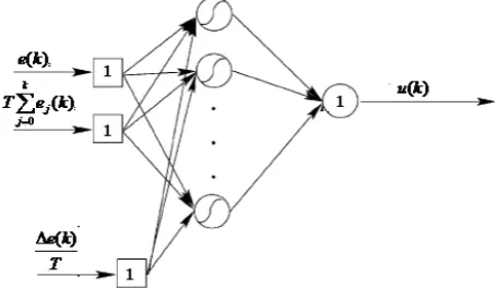
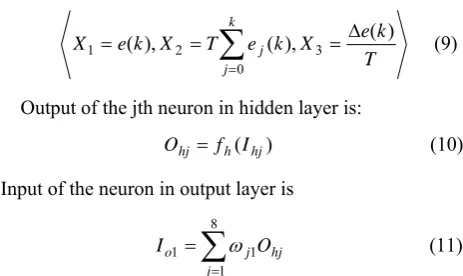
Feed-forward ANN is used to construct an ANN-PID controller. Generally, a three layered feed-forward ANN with appropriate network structure and weights can approach to any random continuous function. The ANN is designed with three layers in consideration of the control system real time requirement. Obviously, there are three nodes in input layer, the deviation e(k), the cumulation of deviation ej(k) and the variety of deviation

Δe(k) . Only one node in output layer, that is, the output of the controller u(k). In order to simplify the structure of the ANN, hidden layer nodes, which can correctly reflect the relationship between the input and the output of the ANN, are designed as few as possible, and 8 nodes is assumed in this paper. In practice, hidden layer nodes can be acquired by experiment or experience [4][15][16]. The neuron activation function of input layer is assumed linear function fi(x) =x; that of hidden layer is assumed the Sigmoid function fh(x)=1/(1+e-x) and that of output layer is assumed linear function fo(x)=x. So a 3-8-1 network is constructed and is shown in Fig. 1, which can take the place of traditional PID controller.

In Fig.1, the ANN-PID three inputs of input layer

are ek T e k e

( )

k T

k

j

j Δ

∑

= , ) ( ), (

0

, u(k) is the output of

ANN-PID.

ANN-PID controller generally adopts steepest descent method to learn weights based on the objective function J.

[

( 1)

(

1

)

]

2

1 _{+ − +}

= y k yk

J _p (3)

Where, yp is the desired output of the controlled object at step k+1, y is the actual output of the controlled object at step k+1.

As we all know, using gradient descent method to train

ANN leads to falling into local minimum and slowing speed of converge, therefore in order to get ride of this defect, in next section, the different evolution algorithm (DEA) is adopted to train weights of the ANN-PID.

III.THE DIFFERENTIAL EVOLUTION AL GORITHM The different evolution algorithm (DEA) is a branch of the evolution algorithms, which has been developed by Storn and Price [17]. DEA is a simple evolutionary algorithm that creates new candidate solutions by combining the parent individual and several other individuals of the same population. A candidate replaces the parent only if it has better fitness. This is a rather greedy selection scheme that often outperforms traditional EAs. Like the other EA, utilizes N, n-dimensional parameter weight vectors wi,G, i = 1, . . ., N, as a population for each iteration, called generation, of the DEA algorithm. The initial population is taken to be uniformly distributed in the search space. At each iteration, the mutation and crossover operators are applied on the individuals, and a new population arises. Then, the selection phase starts, where the N best points from both populations are selected to comprise the next generation.

According to the mutation operator, for each weight vector, wi,G, i = 1, . . ., N, a mutant vector is determined through the equation:

Vi,G+1=Wr1,G+F•

(

Wr2,G−Wr3,G

)

(4)

Figure 2. The ANN-PID control system based on DEA. .

greater than or equal to 4, in order to apply mutation. Following the mutation phase, the crossover operator is applied on the population, combining the previously mutated vector,vi,G+1=[v1i,G+1,v2i,G+1,…,vDi,G+1] with a so- called target vector, wi,G+1=[w1i,G+1,w2i,G+1,…,wDi,G+1]. Thus a so-called trial vector, ui,G+1=[u1i,G+1,u2i,G+1,…, uDi,G+1] is generated, according to

u

ji_,G₊₁

=

V

ji_,G₊₁, if (Randb(j)≤CR)orj=rnbr(i) (5)

or

u

_ji,G+1

=

V

_ji,G+1, if (Randb(j)>CR) or j≠rnbr(i) (6)

where i = l, . . ., N, randb(j)∈[0, 1] is the jth evaluation of a uniform random number generator, for j∈1, 2, . . ., D, and rnbr(i) ∈1, 2, . . ., d is a randomly chosen index. CR∈[0, 1] is the crossover constant (user defined), a parameter that increases the diversity of the individuals in the population. The three algorithm parameters that steer the search of the algorithm are the population size (N), the crossover constant (CR) and the differential variation factor (m). They remain constant during an optimization. To decide whether or not the vector ui,G+1 should be a member of the population comprising the next generation, it is compared to the initial vector wi;G. Thus,

(

) ( )

⎪⎩ ⎪ ⎨

⎧ < = + +

+

otherwise w

w f u

f u w

G i

G i G

i G i G

i _,

,

,

, 1

, 1 , 1

, (7)

The procedure described above is considered as the standard variant of the DE algorithm. Different mutation and crossover operators have been applied with promising results. In addition, DE algorithms have a property that Price has called a universal global mutation mechanism or globally correlated mutation mechanism, which seems to be the main property responsible for the appealing performance of DE as global optimizers.

To apply DEA algorithms to ANN training weights as an initial weight population, and evolve them over time; N is fixed throughout the training process, and the weight population is initialized randomly following a uniform probability distribution.

At each iteration, called generation, new weight vectors are generated by the combination of the weight vectors randomly chosen from the population. This operation is called mutation. The derived weight vectors are then mixed with another predetermined weight vector, the ‘‘target’’ vector, through the crossover operation. This operation yields the so called trial vector. The trial vector is accepted for the next generation if and only if it reduces the error value of the objective function J ((3)). This last operation is called selection. The above-mentioned operations introduce diversity in the population and are used to help the algorithm escape the local minima in the weight space. The combined action of mutation and crossover is responsible for much of the effectiveness of DEA’s search, and allows them to act as parallel, noise-tolerant, hill-climbing algorithms, which efficiently search the whole weight space [22][23].

IV.THE ANN-PID LEARNING ALGORITHM BASED ON THE DEA

As shown in the following Fig. 2, ANN-DEA-PID is controller based on the artificial network and the different evolve algorithm, r is system referenced input, y is system output, u is controlling output of ANN-DEA-PID controller. Deviation e, cumulation of deviation Σe and variety of deviation Δe are applied as the inputs of ANN-DEA-PID controller. In this control system, we adopt the hybrid method combined of differential evolution algorithm and steepest descent algorithm for ANN-DEA-PID. The DE algorithm works on the termination point of steepest descent algorithm. Thus the method consists of a steepest descent strategy-based ANN-DEA-PID training stage and a differential evolutionary strategy-based ANN-DEA-PID retraining stage.

A. First Stage: the Steepest Descent Algorithm for ANN-DEA-PID

The proposed learning procedure is based on the gradient descent learning rule for ANNs learning. In Fig.1, Input layer’s weights are 1,T,1T . Input of

hidden layer’s jth neuron can be written as follows:

∑

=

= 3

1

i i ij

hj X

I ω (8)

Where ωij is the weight which connect jth(j=1,2…8) neuron in hidden layer with ith(i=1,2,3) neuron in input layer; Xi (i=1,2,3) are the outputs of input layer, that is:

T k e X k e T X k e X

k

j j

) ( ,

) ( ),

( ₃

0 2 1

Δ = =

=

∑

=

(9)

Output of the jth neuron in hidden layer is:

Ohj = fh(Ihj) (10) Input of the neuron in output layer is

∑

=

= 8

1 1 1

j

hj j

o O

I ω (11)

Oo₁= fo(Io₁)=Io₁ (12)

Output of the neutral network PID controller is

1 1 1 ( ) )

(k Oo fo Io I_o

u = = = (13) 1) Adjusting of Output Layer’s Weights

Weight learning rule is

1 1 j j J ω η ω ∂ ∂ − =

Δ (14)

Where η is learning speed, it commonly is (0, 1).

(

)

) ( ) 1 ( ) 1 ( ) 1 ( ) 1 ( ) 1 ( ₁ 1 1 1 k u k y O k y k y O O k y k y J J hj p j o o j ∂ + ∂ + − + − = ∂ ∂ ∂ + ∂ + ∂ ∂ = ∂ ∂ ω ω (15)

where ∂y(k+1) ∂u(k) is unknown which denotes system’s input-output relationship. For most systems, its signal is definite. ∂y(k+1) ∂u(k) is replaced withsgn(∂y(k+1) ∂u(k)), and learning speed η is used to equalize the calculate error. Adjusting rule of output layer’s weights ωj1 is:

₍

₎

) ) ( ) 1 ( sgn( ) 1 ( ) 1 ( ) ( ) 1 ( ₁ 1 k u k y O k y k y k k kj p j j ∂ + ∂ + − + + = + η ω ω (16)

2) Adjusting of Hidden Layer’s Weights Weight learning rule is

(

hj

)

i hj hj i hj hj hj i hj ij hj hj ij ij X O O O J X I O O J X I J I I J J − ⎟ ⎟ ⎠ ⎞ ⎜ ⎜ ⎝ ⎛ ∂ ∂ − = ⎟ ⎟ ⎠ ⎞ ⎜ ⎜ ⎝ ⎛ ∂ ∂ ∂ ∂ − = ∂ ∂ − = ∂ ∂ ∂ ∂ − = ∂ ∂ − = Δ 1 η η η ω η ω η ω (17) 1 8

1 1 1

1 1 1 j i o hj j hj o hj o o hj I J O O J I J O I I J O J ω ω

∑

= ∂ ∂ = ∂ ∂ ∂ ∂ = ∂ ∂ ∂ ∂ = ∂ ∂

(

)

) ( ) 1 ( ) 1 ( ) 1 ( ) 1 ( ) 1 ( 1 1 1 k u k y k y k y O k y k y J j p j o ∂ + ∂ ⋅ + − + − = ∂ + ∂ + ∂ ∂ = ω ω (18)

wher∂y(k+1) ∂u(k)is replaced by sgn(∂y(k+1) ∂u(k)),

learning speed η is used to equalize the calculate error. Corresponding adjusting rule of hidden layer’s weights ωij is:

(

)

(

)

) ) ( ) 1 ( sgn( 1 ) 1 ( ) 1 ( ) ( ) 1 ( 1 k u k y X O O k y k y k k i hj hj j p ij ij ∂ + ∂ − + − + + = + ω η ω ω (19)

A generic description of the proposed hybrid algorithm is given in Algorithm 1.

Algorithm.1

Stage 1: the steepest descent learning 

Step 1a: Decide network structure at first. Because the nodes of network input layers and output layers are known, only the nodes of hidden layers remained undecided.

Step 2a: Initialize the weights of hidden layers ωij and the ones of output layers ωj1with less random number, select the speed of learning η;

Step 3a: Repeat for each input concept state (k). Step 4a: Sample the system,

get T k e k e T k e k j j ) ( , ) ( ), ( 0 Δ

∑

=

, which are the

network inputs;

Step 5a: According to formula (9) and (11) calculate the outputs of hidden layer and output layer, get the controlling amount u;

Step 6a: Calculate the system output and get y(k +1) ; Step 7a: According to the weights adapting rule (15) and

(18) of output layer and hidden layer, regulate each connection weight of output layer and hidden layer.

Step 8a: Calculate objective function J

Step 9a: Until the termination conditions are met.

Step10a: Return the final weights WSDA (k+1) to the Stage 2.

Stage 2: the differential evolution learning

Step 2b: Initialize the DE population in the neighborhood of WSDA (k+1) and within the suggested weight constraints (ranges).

Step 2b: Repeat for each input concept state (k). Step 3b: For i = 1 to NP.

Step 4b: MUTATION (wi(k) )→Mutant_Vector.

Step 5b: CROSSOVER (Mutant_Vector)→Trial_Vector. Step 6b: If J (Trial_Vector)≤ J(wi(k) ), accept Trial_Vector

for the next generation. Step 7b: End For.

Step 8b: Until the termination condition is met.

First, the steepest descent algorithm is outlined in the Stage 1 of Algorithm 1, and provides convergence of concepts’ values in a desired state. The key features of the steepest descent algorithm method are the low storage requirements and the inexpensive computations. In Stage 2 of Algorithm 1, the differential evolution (DE) algorithm, responsible for the ANN-DEA-PID retraining is outlined.

n-Figure 3. The ANN-PID control system based on DEA. dimensional weight vectors, as initial population, and

evolve them over time; N is fixed throughout the training process, and the weight population is initialized by perturbing the appropriate solution provided by the steepest descent algorithm. Also, the appropriate fitness function is determined. In this case, the steepest descent algorithm seeds the DE, i.e. a preliminary solution is available by the steepest descent algorithm; so, the initial population might be generated by adding normally distributed random deviations to the nominal solution. However, in the experiments reported in the next section, we have also used the constraints on weights defined initially by experts to perturb the approximated solution provided by steepest descent algorithm.

Let us now give some details about the version of DE algorithm used here. Steps 4b and 5b implement the mutation and crossover operators, respectively, while Step 6b is the selection operator. For each weight vector wi(k) the new vector called mutant vector is generated according to the following relation:

Mutant vector

(

)

NP

i w w w w w

v

r r k i k best k

i k i

L 2 , 1

, 2 1 ) ( ) ( )

( ) 1 (

=

− + − ⋅ + = = +

μ (20)

Where wbest(k) is the best population member of the previous iteration, μ>0 is a real parameter (mutation constant) which regulates the contribution of the difference between weight vectors, and wr1, wr2 are weight vectors randomly chosen from the population with r1, r2 {l, 2, . . ., i∈ -l, i+1, . . ., N}, i.e. r1, r2 are random integers mutually different from the running index i. Aiming at decreasing the diversity of the weight vectors further, the crossover-type operation yields the so-called trial vector, ui(k+1), i = 1, . . ., N. This operation works as follows: the mutant weight vectors (vi(k+1), i = 1, . . ., N) are mixed with the ‘‘target’’ vectors, wi(k+1), i = l, . . ., N. Specifically, we randomly choose a real number r in the interval [0, 1] for each component j, j = 1, 2, . . ., n, of the vi(k+1) . This number is compared with CR [0, ∈ 1](crossover constant), and if r≤CR; then, the jth component of the trial vector ui(k+1), gets the value of the jth component of the mutant vector vi(k+1) ;otherwise, it gets the value of the jth component of the target vector, wi(k+1). The trial vector is accepted for the next generation if and only if it reduces the value of the following proposed fitness function J; otherwise the old value, wi(k+1) is retained. This last operation is the selection, and due to the moving ‘‘optimum’’ nature of the differential evolution task, it ensures that the fitness J starts steadily decreasing at some iteration. Here, clearly, the fitness function J is formula (3).

The purpose is to determine the values of the weights of the ANN-DEA-PID that produce a desired behavior of the system. The determination of the weights is of major significance and it contributes towards the establishment of ANN-DEA-PID as a robust methodology, and improves the performance of ANN-DEA-PID.

V.SIMULATION ANALYSIS

The neural network PID controller with the differential evolutional algorithm, which is proposed in this paper, is a constructed by neural network PID controller and the differential evolutional algorithm. In this new PID controller, the artificial neural network is used to approach the conventional PID formula and the differential evolution algorithm (DEA) is used to search weight of the artificial neural network.

Five examples with different complexity levels are described in this section and are used for the simulations.

A. First Order System

The first example is the first order systems model as follow

1 95

1 ) (

+ =

s s

G (21)

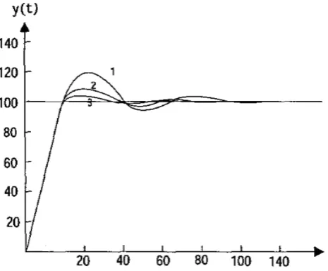
For this delay time system, the parameters are chosen as follow: sample period Ts= 1s, reference value r= 100, the traditional PID controller parameters are Kp=23,Ki =1.375,Kd=0.002. The output response obtained is shown in Fig. 3 as curve 1 for step input signal.

Curve 2 in Fig.3 shows the result of ANN-DEA-PID controller with the 3-8-1 neural network and ANN’s learning speed is 0.1.

Curve 3 in Fig.3 also depicts the output performance of the ANN-PID controller with the 3-8-1 neural network in which the parameters after learning are: Ts, =1s, r = 100,and ANN’s learning speed is 0.1.

B. First Order System with Time Delay

The second example is the first order systems with the time dealy model as follow

1 95 )

( 10

+ = −

s e s G

s

Figure 4. The control effect of PID, ANN-PID and ANN-DEA-PID controller for second order system with time delay. Figure 6. The control effect of PID, ANN-PID and ANN-DEA-PID

controller for first order system with time delay. Figure 5. The control effect of PID, ANN-PID and ANN-DEA-PID

controller for second order system.

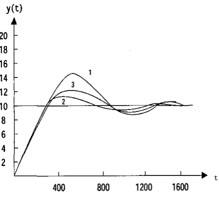
For this delay time system, the parameters are chosen as follow: sample period Ts= 1s, reference value r= 100, the traditional PID controller parameters are Kp=13,Ki =0.325,Kd=0.008. The output response obtained is shown in Fig. 4 as curve 1 for step input signal.

Curve 2 in Fig.4 shows the result of ANN-DEA-PID controller with the 3-8-1 neural network and ANN’s learning speed is 0.1.

Curve 3 in Fig.4 also depicts the output performance of the ANN-PID controller with the 3-8-1 neural network in which the parameters after learning are: Ts, =1s, r = 100,and ANN’s learning speed is 0.1.

C. Second Order System

The second example is the second order systems with the simple model as follow

) 1 (

1 ) (

+ =

s s s

G (23)

For this second order system, the parameters are chosen as follow: sample period Ts=0.5s, reference value r=8, the traditional PID controller parameters are Kp=3.57,Ki=0.125,Kd=0.012.

The output response obtained is shown in Fig. 5 as curve 1 for step input signal.

Curve 2 in Fig. 5 shows the result of ANN-DEA-PID controller with the 3-8-1 neural network and ANN’s learning speed is 0.1.

Curve 3 in Fig. 5 also depicts the output performance of the ANN-PID controller with the 3-8-1 neural network in which the parameters after learning are: Ts, =1s, r = 100,and ANN’s learning speed is 0.1.

D. Second Order System with Time Delay

The third example is the second order system with time delay. The model of it is obtained as following

₍

₎₍

₎

1 23 1 10 ) (

2

+ + = −

s s

e s

G

s

(24)

For this process, the suitable parameters of conventional PID controller are considered as: sample period Ts = 0.5s, reference value r= 10; Kp = 0.1902, Ki = 0.279, Kd = 0.26628.

The curve of output response that marked curve 1 is shown in Fig 6.

For ANN-PID controller with the 3-8-1 neural network and ANN’s learning speed is 0.1, the output response, called curve 2, is given in the same time.

Curve 3 in Fig.6 gives the result of ANN-DEA-PID controller with the 3-8-1 neural network and ANN’s learning speed η=0.1.

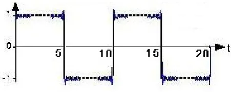
E. the Time Variable Nonlinear System

During the simulation, a typical time variable nonlinear system, which model is

) 1 ( 1

) 1 ( ) 1 ( ) ( )

( 0 ₂

− +

− + − =

k y

k u k y k a k

Figure 7. The control effect of ANN-PID controller for the time variable nonlinear system.

Figure 8. The control effect of ANN-DEA-PID controller for the time variable nonlinear system.

⎟ ⎠ ⎞ ⎜ ⎝ ⎛ + =

25 sin 1 . 0 1 ) (

0 k kπ

a (25)

It is taken as the controlled object. Obviously, the conventional PID controller can not be applied to time variable nonlinear system such as (24).

In here, The ANN-DEA-PID controller with the 3-8-1 neural network structure and the traditional ANN-PID controller are applied respectively. When the input signal is square wave with amplitude is [-1 ,1] and period is 10s.The control system sample period is Ts=0.05s, the corresponding response curves are shown in Fig.6 and Fig.7.

From Fig.7 and Fig.8, it is obvious that the control effect of ANN-DEA-PID controller better than ANN-PID controller and the ANN-DEA-PID controller is more independent and adaptable on the model of the controlled object. This also exactly reflects the outstanding learning and retaining ability and self-adapting ability of neural network. In addition, the different evolve algorithm is adopted to train weights of network, which promotes the performance of the control system and decrease calculated load.

VI.CONCLUSION

The advantages of the ANN-PID controller based DEA are summarized as following:

1. The mathematics model for the controlled object is not necessary;

2. The structure of the controller and the algorithm is simple, and it is convenient to apply them to online real-time control;

3. It is more robust. The method can be applied to industrial process control, and take full advantage of both neural network and traditional PID.

4. ANN-PID controller based on DEA convergence speed is faster than ANN-PID controller and ANN-DEA-PID controller can reach global minimum, due to adopt the different evolutional algorithm to train weight of neural network.

REFERENCES

[1] Yu Yongquan, Huang Ying and Zeng Bi, “A PID Neural Network Controller,” Proceeding of the International Joint Conference on Neural NetWorks, IEEE Copmuter Society Press,California, vol. 3, pp. 1933-1938, 2003.

[2] Yue Pan,Ping Song and Kejie Li, “PID Control of Miniature Unmanned Helicopter Yaw System based on RBF Neural Network,” Intelligent computing and Information Science,vol. 135,pp. 308-313,2011.

[3] Haiquan Wang, Dongyun Wang and Guotao Zhang, “Research of Neural network PID Control of Aero-engine,” Advances Automation and Robotics, vol. 1, pp. 337-343, 2010.

[4] Iwasa,T.,Morizumi,N.andOrmatu,S. “Temperature Control in a Batch Process by Neural Networks,”Proceeding of IEEE World Congress on Computational Intelligence, IEEE Press,New York, vol. 2, pp. 992-995, 1992.

[5] Li qi, Li shihua. “Analysis and Improvement of a Kind of neural Networks Intelligent PID Control Alogrithm,” Control and Decision Editorial Department, ShenYang China, vol. 13, pp. 311-316, 1998.

[6] Moradi,M.H. “New Techniques for PID Controller Design,” Proceeding of 2003 IEEE Conference on Control Applications, IEEE Press,New York, vol. 2, pp. 903-908, 2003.

[7] Indranil Pan,Saptarshi Das,Amitava Gupta, “Tuning of an optimal fuzzy PID controller with stochastic algorithms for networked control systems with random time delay,” ISA Transaction, vol. 50, pp. 28-36, 2011.

[8] G.jahedi, M.M.Ardehali, “Genetic algorithm-based fuzzy-PID control methodologies for enhancement of energy efficiency of a dynamic energy system,” Energy Conversion and management, vol. 52, pp. 725-732,2011. [9] T. Back,H.P. Schwefel. “An overviewof evolutionary

algorithms for parameter optimization,” Evol. Comput., pp. 1–23,1993.

[10] N. Dodd, “Optimization of network structure using genetic techniques,” in Proceedings of the 1990 International Joint Conference on Neural Networks, 1990.

[11] P. Bartlett, T. Downs, “Training a Neural Network Using a Genetic Algorithm,” Tech. Report, Department of Electrical Engineering, University of Queensland, 1990. [12] H.G. Beyer, H.P. Schwefel, “Evolution strategies: a

comprehensive introduction,” Nat. Comput., vol. 1, pp. 3– 52, 2002.

[13] Saptarshi Das,Indranil Pan,Shantanu Das,etc, “A novel fractional order fuzzy PID controller and its optimal time domain tuning based on integral performance indices,” Engineering Applications of Aritficial Intelligence, online,2010.

[14] I.L. Lopez Cruz, L.G. Van Willigenburg, G. Van Straten, “Efficient differential evolution algorithms for multimodal optimal control problems,”Application Soft Computing,vol. 3, pp. 97–122,2003.

[15] G.D. Magoulas, V.P. Plagiannakos, M.N. Vrahatis, “Neural network-based colonoscopic diagnosis using on-line learning and differential evolution,” Appl. Soft Comput., vol. 4, pp. 357–367, 2004.

neural network based model predictive control (NNMPC): An experimental investigation,” Control Engineering Practice, vol. 19, pp. 454-467, 2011.

[17] R. Storn, K. Price, “Differential evolution: a simple and efficient heuristic for global optimization over continuous spaces,” J. Global Optimization, vol.11, pp. 341–359, 1997. [18] G. Weiss, “Towards the synthesis of neural and

evolutionary learning,” in: O. Omidvar (Ed.), Progress in Neural Networks, 5, Ablex Pub, 1993 Chapter 5.

[19] G.Weiss, “Neural networks and evolutionary computation, partI: hybrid approaches in artificial intelligence,” in: Proceedings of ICEC, 1993.

[20] G.Weiss, “Neural networks and evolutionary computation, part II: hybrid approaches in neurosciences,” in: Proceedings of the IEEE World Congress on Computational Intelligence, 2009.

[21] J. Zurada, “Introduction to Artificial Neural Systems,” WestPublishing Company, 1992.

[22] I.L. Lopez Cruz, L.G. Van Willigenburg, G. Van Straten, “Efficient differential evolution algorithms for multimodal optimal control problems,” Appl. Soft Comput., vol. 3, pp. 97–122, 2008.

[23] Elpiniki I. Papageorgiou, Peter P. Groumpos, “A new hybrid method using evolutionary algorithms to train Fuzzy Cognitive Maps,” Applied Soft Computing, vol.5, pp. 409–431, 2005.

[24] R. Storn, K. Price, “Differential evolution: a simple and efficient euristic for global optimization over continuous spaces,” J.Globalptimization, vol.11, pp. 341–359, 1997. [25] Shu Huailin, “PID Newral Network Control forComplex

Systems,” Processdings of InternationalConference on

Computational Intelligence for Modelling, Control and Automation CCIMCA 99’2,10s Press, 1999, pp. 166-171. [26] Shu Huailin, “Analysis of PID Neural Network

Multivariable Control Systems,” ACTA Automatica Sinica, vol.25, pp. 105-111, 2008.

[27] K.V. Price, “An introduction to differential evolution,” in: D.Corne, M. Dorigo, F. Glover (Eds.), New Ideas in ptimization, McGraw-Hill, New York, 1999.

[28] J.C.F. Pujol, R. Poli, “Evolving the topology and the weights ofneural networks using a dual representation,” Appl. Intell., vol.8, pp. 73–84, 2010.

[29] H.P. Schwefel, “Numerical Optimization of Computer models,” Wiley, Chichester, 1981.

[30] H.P. Schwefel, Evolution and Optimum Seeking, Wiley, NewYork, 1995.

[31] R. Storn, “On the Usage of Differential Evolution for Function Optimization,” NAFIPS, Berkely, pp. 519–523, 1996.

[32] R. Storn, K. Price, “Minimizing the real functions of the ICEC’96 contest by differential evolution,” in: Proceedingsof the IEEE Conference on Evolutionary Computation, Nagoya, pp. 842–844,2009.

[33] A. Tiwari, R. Roy, G. Jared, O. Munaux, “Evolutionary-based techniques for real-life optimization: development and testing,” Appl. Soft Comput., vol.1, 2002, pp. 301–329. [34] J. H. Kim, K.K.Choi, “Self-turning discrete PID

Controller,” IEEE Trans. Indst. Electron., vol.34, pp. 298-300. 2007.