DOI 10.1007/s13173-010-0024-0 O R I G I N A L PA P E R
Application oriented connected dominating set-based cluster
formation in wireless sensor networks
V.S. Anitha·M.P. Sebastian
Received: 3 February 2010 / Accepted: 21 November 2010 / Published online: 3 December 2010 © The Brazilian Computer Society 2010
Abstract Clustering is a fundamental mechanism used in the design of Wireless Sensor Network (WSN) protocols. The performance of WSNs can be improved by selecting the most suitable nodes to form a stable backbone struc-ture with guaranteed network coverage. This paper pro-poses a base station-controlled centralized algorithm for sta-tic sensor networks and a distributed, weighted algorithm for dynamic sensor networks. The solutions are based on a (k, r)-Connected Dominating Set, which is suitable for cluster-based hierarchical routing. The clusterhead redun-dancy parameter k improves reliability, the multi-hop pa-rameterr addresses the scalability issue and the combined weight metric improves the network lifespan and reduces the number of re-affiliations. To create a stable and efficient backbone structure, the backbone sensor nodes are selected based on quality, which is a function of the residual battery power, node degree, transmission range, and mobility of the sensor nodes. Simulation experiments are conducted to eval-uate the performance of both the algorithms in terms of the number of elements in the backbone structure, re-affiliation frequency, load balancing, network lifespan, and the power dissipation. The results establish the potential of these algo-rithms for use in WSNs.
Keywords Sensor network·Weighted clustering· Connected dominating set·Load balancing·Mobility
V.S. Anitha (
)National Institute of Technology, Calicut, Kerala, India e-mail:[email protected]
M.P. Sebastian
Indian Institute of Management Kozhikode, Kozhikode, Kerala, India
e-mail:[email protected]
1 Introduction
Development of wireless sensor networks (WSN) is en-abled with the recent technological advancement in wire-less communications, low-power consumption processors, and highly integrated digital electronics. A dense sensor network consists of hundreds or thousands of sensor nodes with capabilities of sensing, processing, and communicat-ing and are deployed in uncontrolled hostile environment and for unattended operations. A WSN typically has little or no infrastructure. The two approaches to deploy sensors in a WSN are the deterministic deployment and the ran-dom deployment [24]. In deterministic deployment, sensors are placed exactly at pre-engineered positions, whereas in random deployment, large numbers of sensor nodes are dis-persed randomly by dropping from a plane or throwing from a moving vehicle. Failures are inevitable in WSNs as the battery-drained nodes create holes in the network topology, causing connectivity and information loss. Therefore, use of energy-aware algorithms with failure detection and mainte-nance mechanism is crucial in the design of WSNs.
A wireless system is expected to support ‘anytime any-where’ type of service and this characteristic makes it a very attractive technology. A cellular telephone system provides a connection to the Public Switched Telephone Network (PSTN) for any user within the radio range of the system. The available bandwidth of cellular radio systems is low and it allow voice and data communication through hand-held phones. Bluetooth allows users to make ad hoc wire-less connections between devices like mobile phones, desk-top, or notebook computers without any cable. It supports uni-cast and multi-cast connections and uses the concept of master and slave. A device needs to wait until the master allows it to talk.
mobile nodes. Among the existing wireless ad hoc network models, Mobile Ad hoc Networks (MANETs) are closely related to WSNs. They share some common characteristics, such as wireless communication media, the network topol-ogy and, bandwidth and energy constraints. Hence, many existing concepts, protocols and techniques used in cellu-lar, Bluetooth, MANET, and traditional wireless networks are applicable to WSNs, also. But some unique features and applications of WSNs make them different from the other wireless networks. The unique characteristics of a WSN in-clude data-centric nature of the network, physical resource constraints, environment-driven nature, and the correlated data problem. Energy conservation is a more relevant mat-ter than capacity for most of the sensor network applica-tions [10]. Also, in generic, the WSN nodes are deployed densely than in MANETs. These features together with the wide ranges of application requirements necessitate the de-sign of new or modified protocols for WSNs.
The Sensor network applications include, but are not lim-ited to (i) military and civilian applications (e.g., battle field surveillance, sensing of intruders, reconnaissance, and tar-geting systems); (ii) academic, industrial, and home appli-cations [22,26] (e.g., automotive manufacturing, monitoring product quality, managing inventory, and home automation); (iii) physical world applications [1,8,9,20,23] (e.g., envi-ronmental monitoring like early fire detection in forests, de-tection, and monitoring of environmental changes in oceans and plains, chemical, or biological detection and flood de-tection); and (iv) health applications [28,33] (e.g., monitor-ing and assistmonitor-ing of patients and drug administration). Most WSN applications require scalability, load balancing, and prolonged network lifetime. The use of networked system of sensors can limit the chance for personal interaction in the usually dangerous reconnaissance missions [3].
2 Background
The concept of virtual backbone infrastructure is used by researchers for broadcasting, area monitoring and process scheduling. Keeping a battery operated sensor node always active is not desirable as it quickly depletes its energy re-sources. The lifetime of a sensor node can be extended if it uses energy only during the specified time slot allotted to it. Thus, every sensor node must turn off its circuitry to con-serve energy when its time slot has passed. The concept of a backbone structure to the sensor network allows some of the nodes to be off when not in use. This saves power and prolongs the network lifetime. However, to support the com-munication efficiently, the members of the backbone need to be always active and stable. Hence, the selection of the backbone members must be done judiciously.
A Connected Dominating Set (CDS) serves as a virtual backbone for WSNs to reduce the routing overhead [27].
A Dominating Set, DS, is defined as a set of nodes in the network such that all nodes in the network which are not in the DS are adjacent to at least one node in the DS. When the graph induced by a DS is connected, then it is called a CDS. For any arbitrary network, the problem of computing the CDS of minimum cardinality is an NP-complete prob-lem [18].
CDS-based clustering of sensor nodes into groups allow sensors communicate information to the Sink through the stable backbone nodes. This saves considerable amount of energy and helps in prolonging the network lifespan. Other than to support network scalability and power efficiency, clustering conserves communication bandwidth, and stabi-lizes the network topology. The topology of a sensor net-work influences its latency, robustness, and data aggrega-tion capability. Flooding for broadcasting purpose can cause broadcast storms. Therefore, recent broadcasting, activity scheduling, and area monitoring algorithms use the concept of virtual network infrastructure known as backbone struc-ture (B-strucstruc-ture). The construction of a stable B-strucstruc-ture offers better support for efficient communication. The back-bone is a subset of the sensors that perform data communi-cations and serves the nodes that are not part of the back-bone [29]. A previous research work [30] has shown that the backbone reduces the routing overhead dramatically. A vast literature about the backbone construction can be found in [31]. Cluster-based routing is a special case of backbone-based routing with the nodes in the backbone considered to be clusterheads [14].
This paper proposes centralized and distributed solutions for creating and maintaining B-structures for static and dy-namic WSNs, respectively. These algorithms are based on a (k, r)-CDS and the nodes for the construction of the B-structure are elected based on the residual battery power, node degree, transmission range, and mobility. To provide redundancy, the CDS is constructed in such a way that any sensor node is covered by at leastkbackbone nodes within ther-hopdistance. The proposed clustering schemes enable the formation of stable clusters and use techniques to main-tain the cluster structure as stable as possible with minimal control messages. To adhere to the cluster-based approach, after constructing the virtual backbone with CDS members, clusters are created with CDS members as clusterheads. Even though our proposals avoid the necessity for network wide synchronization, clusterheads allow its members to switch to the low power sleep mode through the schedul-ing mechanism. This schedulschedul-ing is in the round-robin order. Duty-cycling is achieved by selecting only a subset of the nodes in WSN (the CDS members, in this case), to remain active for communication and control.
for learning the network topology and grows with the net-work size. Hence, it is suitable for static and known topology networks. The distributed algorithm creates stable, scalable, and load balanced B-structure, which can be used for large and dynamic topologies.
The rest of the paper is organized as follows. Section2 re-views the previous works while Sect.3describes the system model and the performance parameters. Section4presents the design of the proposed protocols. Section5evaluates the performance of the protocols, and Sect.6concludes the pa-per.
3 Related work
A sensor network can be considered as an embedded system which has self-configuration, self-healing, multi-hop com-munication, and dynamic routing. A survey on the design issues, applications, and techniques for WSNs is presented in [4]. Routing in sensor networks got lot of attention in the recent years. A survey on the routing issues and techniques in WSNs is presented in [2]. Grouping of sensor nodes into clusters has been studied extensively for achieving network scalability, energy efficiency, and stability. Low energy con-sumption is a critical design requirement for WSN applica-tions. Efficient routing techniques play a major role in the energy consumption and maximize the lifetime of a sensor network.
Low Energy Adaptive Clustering Hierarchy (LEACH) [21] is one of the most popular clustering algorithms for WSNs. It creates clusters based on the received signal strength and uses clusterhead nodes to route packets to the Sink. The role of the clusterhead is rotated periodically among the nodes of the cluster in order to balance the load. The clusterhead election normally does not take care of the capability of a node to act as clusterhead, and hence a node with low residual battery power may be selected as cluster-head. Also, such elections cannot be applied to large sensor networks. Power Efficient Gathering in Sensor Information Systems (PEGASIS) [25] is a greedy algorithm and is power efficient. However, it does not scale well and is not applica-ble to sensor networks with unknown topologies.
Hybrid Energy Efficient Distributed Clustering (HEED) [37] is an energy efficient, hybrid, and distributed clustering algorithm. It periodically selects a clusterhead based on the residual energy and communication costs. It needs multiple broadcasting for cluster formation, thus consumes more en-ergy. Distributed Weight-based Energy Efficient Hierarchi-cal Clustering [16] proceeds in a distributed manner. It aims at generating balanced cluster sizes and needs significantly low energy consumption in inter and intra-communication than HEED. The connected dominating set concept was first introduced by Guha and Kuller [19]. They have proposed
three centralized, greedy approximation algorithms. The al-gorithm proposed by Das et al. [15] first computes the dom-inating sets and then additional nodes are added to covert the DS into connected DS. The algorithm proposed by Wu and Li [34] first constructs a connected dominating set and then deletes the redundant nodes based on some rules. The performance ratio is not given with the proposal. Wan et al. [32] proposal requires the construction of a spanning tree to select the dominating nodes. Distributed Solutions for computing approximations to the minimum CDS prob-lem have been proposed in [12] and [13]. To improve power efficiency, stability, and network lifetime, along with the re-duction in the total number of dominating nodes, the quality of these dominating nodes is also to be considered.
Some approximation algorithms have been proposed to construct the k-connected m-dominating set (kmCDS) to improve the fault tolerance and routing flexibility. The pro-tocol [36], first constructs them-dominating set and then makes it tok-connected by augmenting the first. The mes-sage complexity of this approach is very high. Wu and Li [35] proposed a distributed algorithm with low message complexity to construct a kmCDS for generic values ofk andm. This approach requires a high degree of redundancy for the network topology. The major design objective of the dominating set-based/Connected Dominating set-based ap-proach is the construction of a virtual backbone with min-imum number of nodes (the quality of a node to act as a backbone member is not at all considered). As a solution to this problem, a centralized, scenario-based, weighted, and dominating set-based algorithm for mobile ad hoc networks is proposed by the authors in [5]. In [6], the authors have proposed a distributed, adaptive, and weighted clustering al-gorithm for mobile ad hoc networks.
The Weighted Clustering Algorithm (WCA) [11] is a combined weight metric-based clustering approach to form single-hop clusters. In WCA, a node with minimum sum of four indices is elected as the clusterhead. To determine a clusterhead, the algorithm considers the ideal number of nodes that a clusterhead can handle, the sum of distances to other nodes in its radio distance, mobility, and the time it becoming the clusterhead. WCA has improved performance than the other clustering algorithms as it considers many weight factors. All nodes in the network need to compute their weights and should know the weights of other nodes before starting the clustering process. This process takes more time and bandwidth, and delays the cluster formation. Moreover, limiting the cluster dimension to a single-hop re-duces the scalability in a large scale networking environ-ment.
scalable, adaptive, and power efficient with load balancing is not available in the literature. So, in this paper, we propose the design of an adaptive (multi-purpose) clustering proto-col, that is scalable, stable, adaptable, power efficient, and allows load balancing.
4 The WSN model
In this section, we present the WSN model and the design parameters of centralized and distributed scenario-based clustering algorithms.
4.1 The network model
The basic characteristics of any sensor network include dense deployment of sensor nodes, self-organizing capabili-ties, constraints of power and other resources, dynamic net-work topology, mobility of nodes, node failure, multi-hop routing, and short-range broadcast communications. Sensors are deployed in an ad hoc manner in remote or hazardous location without the need for any infrastructure to monitor events and gather data about the environment. The nodes may be static or mobile, homogeneous, or heterogeneous with different energy levels or transmission range.
The sensor network is modeled using a graph G = (V , Et), whereV represents a set of wireless sensor nodes andEtrepresents the connectivity set. Ifu,v∈V then(u, v) ∈Etif and only ifuandvare within the transmission range of each other. The Dominating Set (DS) of graphGis a sub-setM⊆V, such that each node inV not in Mis adjacent to some node inM[7]. A connected dominating set (CDS) for a given graph Gis a dominating set N with the addi-tional requirement that the nodes inN induce a connected subgraph ofG.
The (k, r)-Dominating Set of graph G is defined as a subset D⊆V, such that each node in V not in D is at a distance less than or equal to r from at leastk vertices in D. The(k, r)-CDS,C, is a(k, r)-DSofGwhich induces a connected sub-graph ofG.
Clustering can be modeled as a graph-partitioning prob-lem. The centralized solution for finding(k, r)-CDScan be used if all nodes in the network know the topology of the en-tire network. Distributed solutions are suitable for synchro-nous and asynchrosynchro-nous networks. Nodes in the CDS form the backbone of the sensor network.
4.2 Benefits of(k, r)-CDS-based clustering
The efficiency of multi-cast or broadcast routing can be im-proved through the use of a CDS as backbone. A CDS-backbone eliminates the redundant broadcasts and saves power. It balances the network load and increases the num-ber of nodes in sleep mode. Restricting the routing through
the CDS results in a significant reduction in message over-head associated with routing updates. Reduction in the num-ber of active nodes reduces the end-to-end delay between the Sink and sensor nodes. Most of the CDS-based protocols try to reduce the total number of elements in the backbone structure. This reduction, in turn, reduces the control over-head and the size of the route table. As the backbone nodes coordinate the neighboring ordinary nodes, the increase in the number of ordinary nodes associated with a backbone node increases its overhead. This overload in the backbone causes quick depletion of the residual battery power. Thus, providing clusterhead redundancy for each node in the net-work improves the stability of the backbone. In a CDS based protocol, too much redundancy results in more control over-heads and too little redundancy adversely affects the con-nectivity. The capability of a node to become a clusterhead mainly depends on factors like residual battery power, node degree, transmission range and mobility.
Fault tolerance, reliability, and routing flexibility are nec-essary for efficient routing. Nodes in the WSNs are more prone to failures which may have mobility and with dense population. Thus, it is important to maintain certain degree of redundancy in a CDS. The proposed algorithms use the clusterhead redundancy parameterk to improve reliability, and the multi-hop parameterr to address the scalability is-sues.
4.3 Design parameters
Some characteristics of a node can directly or indirectly in-fluence the efficiency and the rate of control of messages generated by the associated clustering protocol. The prop-erties or metrics, we consider are connectivity, residual bat-tery power, transmission range, and the local stability of the node. These metrics determine the adequacy of nodes to act as clusterheads. In the proposed algorithm, CDS member election is based on a combined weight-metric mechanism. The node weight is the weighted linear combination of the above mentioned metrics, and the weight factors are depen-dent on the service type being deployed in the network. The weight metric can also be an attribute of a single property, but a generalized vision is preferred as ad hoc networks exist in different scenarios and that clustering can be based on dif-ferent priority properties largely depending on the commu-nication scenarios and environment. Different services have different requirements. Depending on the service type, the most important parameters from the service view point are to be considered with high parameter weights, which results in the best suited CDS selection. The node with the highest weight in its neighborhood can be chosen as a member of CDS.
number of nodes within its transmission range. This parame-ter helps to reduce the cardinality of the CDS. A node with high value of transmission power covers a large area, and hence this parameter helps in reducing the total number of clusters in the WSN. Since the clusterheads play the leading role in the communication process, their energy consump-tion is more in comparison with the ordinary nodes. There-fore, a node with sufficient battery power is to be selected as clusterhead to reduce the amount of overhead incurred due to clusterhead re-election and to avoid nodes dropping out of the network prematurely. Certain clustering scenarios de-mand clustering based on the mobility of nodes, and hence the formation of clusters is determined by the mobility pat-tern of nodes to ensure maximum cluster stability.
The processing power, memory capacity, bandwidth, link quality or availability, and transmission rate are also pos-sible parameters which can be considered for the selec-tion of a clusterhead. However, these factors are more rel-evant to MANETs than for WSNs because typical applica-tions of MANETs include non-real time data, multimedia, and voice communication. The typical WSN-applications require transmission of few bytes periodically or upon re-quest or according to some external event. We now discuss the design parameters in detail.
Node degree Each node computes its degree. The degree of a nodevis the total number of nodes within the transmis-sion range ofvand is computed as
Dgv=
u∈V,u=v
{Duv< Tx}, (1)
whereDuv is the distance between nodeuandvandTxis the transmission range.
Residual battery power A node with high residual battery power,Bv, can perform as clusterhead for a longer duration. Hence, computing the residual battery power is a better op-tion than the consumed battery power or the cumulative time during which the node acts as the clusterhead.
Transmission range The transmission range,Tr, of a node is a factor that determines the quality of the clusterhead. This parameter is more relevant in the case of heterogeneous net-works.
The combined weightWv for each nodev∈V is calcu-lated as
Wv=W1∗bv+W2∗dgv+W3∗tr, (2)
whereW1,W2,andW3 are the weight factors for the cor-responding parameters andbv,dgv,andtr are normalized values ofBv,Dgv, andTr, respectively.
Mobility Most of the network architectures assume that the sensor networks are stationary which need not be true. For instance, in a target detecting or tracking application, it is deemed necessary to support mobility of sensor nodes. Sta-bility of a node denotes how stable the node is for being a clusterhead. To compute mobility, each node in the domi-nating set needs to find out the distance from its neighboring nodes. For distance computation, Friis [17] free space prop-agation model is used.
The received power,Pr is computed as
Pr=Pt∗Gt∗Gr∗ λ 2
(4∗π∗D)2, (3)
wherePr is the power received by the receiving antenna, Pt is the power input to the transmitting antenna,Gt andGr are the gains of transmitting and receiving antennas, respec-tively, withλas the wavelength, andDas the distance.Pr is inversely proportional to the square of the distance.
Instead of finding the exact physical location, an approx-imate distance at timet between nodesvanduis calculated using (3) as
Dv,ut =√k Pr
, (4)
wherev∈ dominating setDS, u is an element of the set of neighboring nodes ofv andk is a constant.Dtv,u is the distance betweenv anduat timet. The node mobility sig-nificantly influences the network performance.
Relative mobility betweenvanduindicates whether they are coming closer to or moving away from each other. The relative mobility of nodeuwith respect to nodevat timet is given by
RMv,ut =Dv,ut −Dtv,u−1, (5)
RMv,ut is positive if nodeuis moving away fromvand neg-ative ifu is coming closer tov. The distance fromv tou is measured at certain time interval for T times, and thus RMv,u1 ,RMv,u2 , . . . ,RMv,uT are calculated. The standard de-viation of relative mobility gives the variation of the dis-tances over a time period,T as
SDRM=
1
T T
i=1
(RMi−RM)2, (6)
where
RM= 1 T
RMv,u1 +RMv,u2 + · · · +RMv,uT .
A low value of this is an indication of a stable node. This stability is either due to less mobility or due to group mo-bility (the nodev and all its neighboring nodes move in the same direction with more or less same velocity).lstabis the normalized value ofLSTAB.
The quality of a backbone node,v, is calculated as
Qv=Wv+W4∗lstabv, (7)
whereW4is the weight factor associated with the local sta-bility. Suitable values are assigned toW1, W2, W3,andW4 based on the required application such that W1 +W2+ W3+W4=1. The parameters considered may not con-tribute equally to the quality computation (different weights can thus be given to different parameters based on the sce-nario). For example, if the network is more or less static, then the local stability computation can be eliminated or can assign a very small value to W4. It is possible to consider more than four parameters if found relevant.
5 The proposed protocols
In a based approach, the re-election of the cluster-head and the frequent information exchange among the par-ticipating nodes incur high computation and communica-tion overheads. This is minimized by preserving the cluster structure as stable as possible.
5.1 The centralized connected dominating set-based weighted and adaptive clustering algorithm for sensor networks (CCWACS)
The proposed algorithm assumes that the sensor nodes are stationary and uses a greedy heuristic for the computation of(k, r)-CDS. This mechanism ensures that all sensor nodes in the network other than the nodes in the backbone are cov-ered by at leastkelements in the backbone within ther-hop distance. The two phases of CCWACS are Clustering setup (meant for backbone creation) and Cluster formation.
5.1.1 Clustering setup phase
The Clustering setup phase computes(k, r)-CDS based on the individual node weight heuristics. The nodes in (k, r)-CDS act as the B-structure members. The weight heuristic uses some parameters to find the suitability of the nodes act-ing as the backbone element. The backbone members are elected on the basis of the node degree, the residual bat-tery power and the transmission range. All nodes in the (k, r)-CDSneed not act as clusterheads and those which are not acting as clusterheads act as gateway nodes. The sec-ond phase is the Cluster formation phase where each regular node selects the most suitable node from the backbone as its
clusterhead. From among thekclusterheads, each node se-lects only one node from the backbone structure as its clus-terhead based on its quality, computed using (7). A node in (k, r)-CDSwithout any cluster members attached acts as a gateway. The node mobility is not considered in the Cluster-ing setup phase because it requires more control messages to compute the local stability of all nodes in the network with respect to their neighbors. But the local stability of the backbone member node is considered in the Cluster forma-tion phase. Hence, only the nodes in the B-structure need to compute the local stability. The algorithm for computing the (k, r)-CDSis as follows:
1. Initialize, the status of all nodes in the network as Ordinary.
2. Compute the weight of each node based on the connec-tivity (hellomessages are used for this purpose), trans-mission range and the residual battery power. The node, v, with the highest weight is selected as a member of the backbone structure and thestatusof that node is assigned asClusterHead. Use Node ID for tie breaking.
3. Assign the status of all 1-hop neighboring nodes of v as NominatedCh and modify the relevant fields (i.e., NodeID, Number of nodes within the r-hop distance, weight, number of clusterheads within the r-hop dis-tance,status) of all nodes within ther-hopdistance ofv. 4. Elect the highest weighted, uncovered node with Nomi-natedChas statusand assign its statusas ClusterHead. The Node ID is used for tie breaking.
5. If all nodes withNominatedChasstatusare covered then a node with the highest number of Ordinary nodes as neighbors is selected as ClusterHead. Use the highest weight for tie breaking.
6. The process continues until all nodes (other than the ClusterHead nodes) have been covered by at least k ClusterHeadnodes within ther-hopdistance.
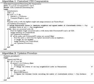
The centralized algorithm for(k, r)-CDScomputation is as shown in Fig.4. The second phase involves cluster forma-tion and management which is common for both central and distributed algorithms and the cluster formation and man-agement issues are discussed in Sect.6.
5.1.2 Example
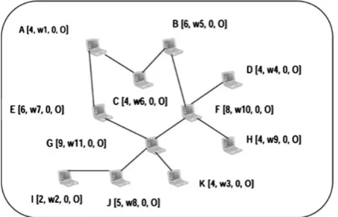
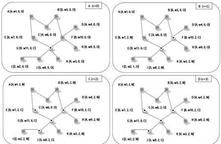
maximum weight is selected as theClusterHead. If there are more nodes with the same weight, tie breaking is done by choosing the lowest-ID. Node G has the highest weight and is thus selected as the clusterhead. All neighboring nodes of G are assigned the status of NominatedCh and all the nodes within the r-hop distance are accounted for the se-lectedClusterHeadas in Fig.2[A].
Node G has four adjacent nodes (E, F, J, and K) and nine nodes at 2-hopdistance. Nodes E, F, J, and K are assigned with status NominatedCh and the third field of all these
Fig. 1 A typical sensor network
nodes is modified accordingly. Among the NominatedCH nodes, node F has the highest weight. Since F is not cov-ered, it is selected as the next node in the backbone and its statusis assigned asClusterHead. All its neighbors are as-signed thestatus NominatedChand the relevant field of the r-hopneighbors is also updated to reflect the new selection as shown in Fig.2[B]. To select the next backbone member, the algorithm searches for an uncovered node withstatus NominatedCh. But in this example, allNominatedChnodes are covered, and hence a NominatedChnode with highest Ordinaryneighbor nodes is to be selected. Here, node B, E, and J have same number ofOrdinaryneighbor nodes. But node J is selected based on its weight (Fig.2[C]). During the next iteration, node E is added to the backbone structure (Fig.2[D]). The algorithm terminates when all the nodes are covered.
5.1.3 Analysis
We now show that the centralized algorithm computes (k, r)-CDS for any connected static network. A wireless sensor network is modeled as a graphG=(V , Et), whereV represents a set of wireless sensor nodes andEt represents the connectivity set. A link exists between two vertices u andvif the Euclidean distance between them is within their transmission range. A connected Dominating Set CDS is a
Fig. 3 Distributed computation of(2,2)-CDS
connected subset ofV ,if all nodes inV −Dare within the r-hopdistance of at leastkelements in CDS.
Theorem 1 The (k, r)-CDS algorithm correctly computes the(k, r)-CDS for any arbitrary connected graph.
Proof Let the network be withnnumber of nodes. All these nodes belong to the setD0r, whereDri means the set of nodes covered by at leastimembers in the connected dominating setC, within the r-hop distance. Initially,C is empty and the elements are added one by one iteratively. The first ele-ment inCis the node with the highest weight. The addition of a new member inC moves one or more members from Dri toDri+1. In case of tie, the node with the lowest NodeID succeeds. In each iteration, a new node is added to the setC. The uncovered nodev, which is a neighbor of any node in C, with the highest weight, is selected in each iteration and v is added to the set C. In the absence of any uncovered NominatedChnodes, the algorithm selects theNominatedCh node with the highest number ofOrdinarynodes as neigh-bors. Sincevis augmented to a connected component,Cis also connected.
Termination: The total number of nodes in the network isnwhich is finite. The algorithm terminates when all the nodes except the members in the backbone are covered by at leastknodes in the ClusterHead node set within ther-hop
distance or all nodes belong to the ClusterHead set. Hence, the total number of iterations is at mostnand the algorithm terminates within a finite amount of time. 5.2 The distributed connected dominating set-based,
weighted, and adaptive clustering algorithm for sensor networks (DCWACS)
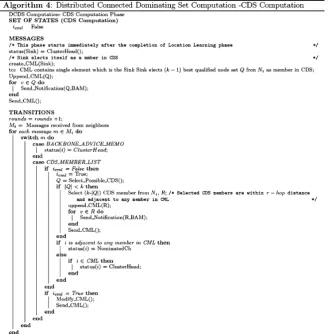
The algorithm assumes that the sensor network is with dy-namic topology. So, DCWACS does not seek the informa-tion about the whole network topology. The nodes need to know only theirr-hopneighborhood. The(k, r)-CDS com-putation is done distributively. The elements in the(k, r)-CDS act as backbone. The distributed algorithm works in two phases, the first phase is the Location learning and the second phase is the CDS-computation.
5.2.1 Location learning
We assume that there is only one Sink (Base Station) and this phase stems from the Sink. In the absence of a Sink, any node in the network with sufficient residual battery power is selected at random to act as the Sink. This phase involves collection of the quality ofr-hopneighborhood and compu-tation of the distance of each node from the Sink.
Fig. 4 Centralized algorithm for(k, r)-CDScomputation
Fig. 6 CDS-computation (DCWACS)
node computes its weight using (2) and sends the Node_Information_Message (NIM) to its r-hop neighbor-hood. In each round, the nodes broadcast the list of avail-able NIM of nodes in ther-hop distance. Afterr rounds, every node in the network learns about itsr-hop neighbor-hood. This phase also computes the distance of each node from the Sink. The Sink initiates this phase by sending a How_Far_Message(HFM) to all its neighbors. On receiving HFM, each node updates the Distance_From_Sink(DIFS) field (which is zero for the initial message from the Sink) and sends this to all its neighbors. If a node gets more than oneHFM, the message with the least value ofDIFStriggers. Every node in the network learns its distance from the Sink in finite amount of time. Thus, at the end of Phase I, each node learns its distance from the Sink and also learns the details of itsr-hopneighbors.
5.2.2 CDS-computation
This phase also starts from the Sink. The Sink elects it-self as a member in the CDS and elects the (k −1)best qualified (based on the degree, residual battery power, and transmission range) immediate neighbor nodes as members of the CDS. Ties are broken choosing the smallest dis-tance. The CDS_MemberList (CML) message containing
the list of elected members is send to its neighbors and the Backbone_Advise_Memo(BAM) to the(k−1)other elected neighbors to notify its selection. Upon receiving theCML, each nodei, selects the backbone elements either from this list or it elects a new member which is adjacent to any one of the members in theCML. This should be within ther-hop distance fromi. This is done only once, immediately after receiving the firstCMLmessage. A node, after electing its backbone elements appends theCMLby adding its elected members to the existing list and transmits the new message to its neighbors. New elections, if any, is intimated through theBAM. The CDS computation continues until all nodes in the network have posted their elections. Appropriate tech-niques are used to eliminate the duplicate messages. The al-gorithm for CDS-Computation is as shown in Fig.6.
5.2.3 Example
Fig.3A, the node G has the highest weight and is elected as the Sink. Afterrrounds, all nodes in the network are fa-miliar with theirr-hopneighborhood. Node G elects(k−1) most qualified nodes as members in CDS. Since thekvalue is 2, node G elects the best qualified adjacent node F as the next member in the CDS. Node G sends the CMLlist to all its immediate neighbors and the Notification to the node F. During the next round, node F changes itsstatusto ClusterHead and all Sink neighbors perform their election process as in (Fig.3B). Thus, nodes E, J, K, and F elect G and F and forward theCMLto its neighbors.
Nodes A, B, D, H, and I are at 2-hop distance away from the Sink. A elects G and E, similarly B, D, and H elect F and G, whereas I elects G and J, as shown in Fig. 3C. In sequence, the next roundCMLreaches to all nodes at 3-hop distance from the Sink and node C elects E and F. This ends the election as all nodes in the network are covered and com-pleted their election processes. The elected backbone ele-ments are E, F, K, and J.
5.2.4 Analysis
Theorem 2 The distributed CDS algorithm correctly com-putes the(k, r)-CDS for any connected graphG.
Proof At the end of the Location Learning phase any node ni in the connected graph knows itsr-hop neighbors,Vrd and the distance to the Sink.
Initialization: Initially, the CDS contains a single node, n0, which is the Sink (a connected, covered subgraph with single noden0).
Maintenance: The node n0 selects the most qualified (with larger weight values) nodes in ther-hopdistance and sends the list of elected members using theCMLmessage. On receiving theCML message, each node starts its CDS member election. This process is done only once and is done immediately after receiving the firstCMLmessage.
The CDS Member election is based on the following rules:
(i) knodes with the highest weight values within ther-hop distance are elected.
(ii) Elected node is either a member inCMLor adjacent to any one element inCML.
Rule (i) preserves the redundancy whereas rule (ii) pre-serves the connectivity. In each round, zero or more number of elements are added to the CDS by nodes in incremental values of the distance from Sink.
Termination: The process repeats until all nodes in the network complete its election. The total number of elements in the network is finite and takes finite amount of time to propagate throughout the network. Hence, the programme terminates within a finite amount of time.
6 Cluster formation and management
The cluster formation procedure starts after building the backbone structure (common for both centralized and dis-tributed algorithms). The backbone members periodically send the Cluster_Head_Advertisement (CHA) to the ordi-nary nodes in the network (each node gets at least k such messages from k different backbone members). A logi-cal relationship pair (NodId,ChId) is established on re-ceiving the first CHA message from ChId. Using t con-tinuousCHAmessages from the dominating set belonging to(NodId,ChId), an ordinary node withNodId computes LSTABand the quality using (7). After computing the qual-ity of all r-hop neighboring backbone elements, an ordi-nary nodeisends Node_Join_Req(NJ) to the most quali-fied member in the backbone. If the total number of nodes attached with that cluster head is below the maximum al-lowable number then the clusterhead accepts this request and sendsNJ_ACK message for confirmation. If the ordi-nary node does not receive anyNJ_ACKmessage within the stipulated time, it sends theNJmessage to the next qualified backbone node within the r-hop distance. Thus, the clus-ters are formed with CDS-members as clusterheads. A CDS member without clustermembers acts as a gateway. To im-prove power efficiency, a clusterhead schedule activities in its cluster so that the nodes can switch to the low-power sleep mode. This scheduling is done in round-robin order.
A good clustering algorithm should preserve the net-work structure as much as possible even when the nodes are moving around and the topology is changing slowly. The clusterhead re-election and the frequent information ex-change between the participating nodes result in high com-putation cost overhead. The proposed algorithms avoid ex-cessive computation in cluster maintenance and the cluster structure be preserved as long as possible. A Cluster man-agement mechanism takes care of the addition of new nodes in the network. Thehellomessage of the new node and the periodicCHAmessage of the CDS member help the cluster head association of the new node.
When a cluster member loses its contact with the cur-rent clusterhead, it selects the next best CDS node from the (k−1)choices as its clusterhead and sends theNJmessage to its new clusterhead. The clusterhead can fail by low bat-tery, by switch off or by fail. When its residual battery is below 20%, a clusterhead informs this message to all clus-ter members so that they can get attached with the next best choice as clusterhead by sending theNJmessage.
uneven energy consumption and shorten the network lifes-pan. The algorithms use techniques to create load balanced clusters.
6.1 Load balancing
The backbone nodes support its members with the radio re-sources and route messages for the other nodes belonging to other clusters. The load handled by a backbone node de-pends on the number of member nodes in its cluster. It is desirable to have uniform load distribution among the back-bone members. It is not practical to share the load with a node whose load is already close to the average network load. We use the Load Balancing Factor (LBF) to quantita-tively measure how well balanced the nodes are. The LBF is given as the inverse of the variance of the load of the nodes, which is computed as
LBF= N i(Li−μ)2
(8)
whereN is the total number of nodes in the network,Li is the load of nodei andμ is the average network load. The average network load is computed as
μ= 1 N
i∈V
Li (9)
It is difficult to maintain a perfectly load balanced network. The LBF value tends to infinity for a perfectly balanced net-work.
The proposed algorithm achieves load balancing by re-distributing the load to different clusterheads based on its quality and by specifying an agreeable threshold on the number of nodes that a clusterhead can handle.
7 Performance evaluation
The performance of CCWACS and DCWACS are evaluated through simulation. The parameters used in the simulation are listed in Table 1. We use a customized simulator in MATLAB. The nodes are randomly placed over a terrain and move according to the Random Waypoint Model. Only the connected topologies are taken into account. An ideal MAC protocol with no collisions is assumed for the simulations as in [32]. As no known optimum solution for the(k, r)-CDS problem in WSN applications is available, the centralized (k, r)-CDSis used as the upper bound in the case of control overhead and lower bound in the case of backbone elements. The centralized algorithm uses many control messages for topology learning and for the(k, r)-CDScomputation but it creates a backbone with optimal number of nodes. The met-rics used for the performance evaluation are (i) Cardinality
of the CDS, (ii) Load balancing Factor, (iii) Number of re-affiliations, (iv) Network lifespan, and (v) Power dissipation. Many CDS-based protocols and algorithms have been proposed in literature. Most of these algorithms are aimed in the construction of Minimum Connected Dominating Set and they create(1,1)-CDS(CDS) or MCDS. Wu and Li pro-posed both centralized and distributed algorithms for CDS construction. Wu and Li’s algorithm computesk-connected, m-dominating set CDS which is closer to our approach than the other popular(1,1)-CDSalgorithms. So, we use Wu and Li’s algorithm for the comparison purposes.
The(k, r)-CDS simplifies the routing by restricting the main routing tasks only to a small number of nodes. The small size(k, r)-CDS reduces the number of nodes in the routing related tasks. Figures7and8show the dependence of r on the number of elements in the backbone structure in centralized and distributed algorithms. As expected, the CCWACS creates a backbone structure with smaller number of nodes than the DCWACS. This is because in CCWACS, a node in the backbone structure is added in such a way that it covers most of the neighbor nodes. Whereas, in DCWACS the elements are added through an election process with the knowledge of ther-hopneighborhood, and hence the subset is not minimal. It can be observed that the number of back-bone elements increases linearly with the number of nodes. In CCWACS, when the bounded distance parameterris in-creased from 1 to 2 there is 16 to 26% reduction in the total number of elements. There is a reduction of 21 to 25% in the backbone structure elements when the value ofris increased from 2 to 3. In DCWACS, there is about 10 to 47% reduc-tion in the number of backbone elements on increasing the value ofrfrom 1 to 2. The rate of reduction is less whenris increased from 2 to 3 (10 to 19%). The backbone elements are elected based on the node weight. As the radius of the election process increases, more nodes select the same set of nodes in their nomination as backbone nodes. Figures9and 10show the comparison of the size of backbone structure
Table 1 CCWACS/DCWACS parameters
Parameter Value
Simulator MAtlab 7.1
Simulation tool Prowler
Number of nodes 50–1000
Network size 100×100 m2, 500×500 m2 Transmission range 10 m–1000 m
Max speed of node movement 10 mtrs/sec W1, W2,W3andW4 0.5,0.3,0.1 and 0.1
Mobility model Random way point
Eelec, Relec 50 nJ/bit
Tamp 100 pJ/bit/m2
Fig. 7 Dependence of r on the number of backbone elements in CCWACS
Fig. 8 Dependence of r on the number of backbone elements in DCWACS
in CCWACS and DCWACS with Wu and Li, respectively. Both CCWACS and DCWACS create backbones with less number of nodes. The reduction in the number of backbone elements is from 20 to 48% in the case of CCWACS and 15 to 28% in DCWACS, in comparison with Wu and Li.
The effectiveness of Load Balancing-heuristics in CCWACS and DCWACS is as shown in Figs. 11 and12, respectively. A higher value of LBF signifies a better load distribution. The load balancing techniques used in these al-gorithms increase the LBF. As the existing alal-gorithms do not support LBS, we do not have a bench mark for comparison purposes.
Figure 13 shows the re-affiliations per unit time in CCWACS with respect to the transmission range. For small values of the transmission range, more number of stable clusters are created, and hence re-affiliations are less. The
Fig. 9 Comparison of cardinality of backbone structure in CCWACS and Wu & Li
Fig. 10 Comparison of cardinality of backbone structure in DCWACS and Wu & Li
number of re-affiliations increases as the transmission range increases. When the transmission range is about 40 meters, the number of re-affiliations takes the maximum value, and further increase in the transmission range leads to less num-ber of re-affiliations. This is because the elected memnum-bers in the backbone structure cover larger areas and the mo-bile nodes tend to stay within this large area. DCWACS also shows similar results. Figure14 shows the comparison of the number of re-affiliations in DCWACS and Wu and Li. It is observed that the number of re-affiliations is much less in DCWACS than in Wu and Li. This is because each ordi-nary node in the network selects the most suitable node as its clusterhead to construct stable clusters.
Fig. 11 Effectiveness of LBF-Heuristics in CCWACS
Fig. 12 Effectiveness of LBF-Heuristics in DCWACS
Sink quickly drain their battery power and drop out of the network. The Minimum-Energy Multi-hop routing (MTE) uses intermediate nodes for communicating with the Sink. Hence, in MTE routing, the nodes near to the Sink are used for routing a large amount of messages to the Sink and die earlier than the nodes far away from the Sink. In CCWACS and DCWACS also, the nodes in the B-structure can com-municate either directly or through multi-hop to the Sink.
The lifetime of a network is the number of rounds com-pleted without a single hole in the network or the number of rounds completed with at least a single active node remain-ing in the network. Table2shows the comparison of the first node death and the last node death for the different proto-cols. In CCWACS-M and DCWACS-M, the first node death is found earlier than in CCWACS-D and DCWACS-D, re-spectively. But the last node dies earlier in CCWACS-D and DCWACS-D than in the corresponding multi-hop transmis-sions. CCWACS and DCWACS (both Direct and Multi-hop)
Fig. 13 Number of re-affiliations per unit time Vs Transmission range
Fig. 14 Comparison of the number of re-affiliations in DCWACS and Wu and Li
Table 2 Lifetimes of the protocols (in number of rounds)
Protocol First node dies (rounds) Last node dies (rounds)
Direct 45 115
MTE 8 212
CCWACS-D 63 418
CCWACS-M 55 479
DCWACS-D 73 465
DCWACS-M 64 514
Wu and Li 51 341
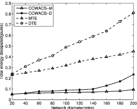
Fig. 15 Total power dissipated using Direct, MTE, CCWACS-D, and CCWACS-M for a random network
Fig. 16 Total power dissipated using Direct, MTE, DCWACS-D, and DCWACS-M for a random network
selected based on its residual battery power, node degree, transmission range, and mobility.
Figures15and16show the total energy dissipated for the scenario in which each node has a 2500 bit packet to send to the Sink. The random network withEelec,RelecandTamp as shown in Table1is used. It is observed that CCWACS-M and DCWACS-CCWACS-M save an average of 70% and 58%, re-spectively, of the total energy dissipated in comparison with MTE. Similarly, CCWACS-D and DCWACS-D save an av-erage of 65% and 60%, respectively, of the of total energy dissipated in comparison with the Direct protocol.
8 Conclusions
In this paper, we have presented connected, dominating set-based, weighted, and adaptive clustering algorithms
(Cen-tralized and Distributed) for ad hoc sensor networks. The elements in the backbone structure are selected based on the (k, r)-CDS. The Centralized-algorithm computes the dom-inating set elements progressively, taking the most suitable sensor node based on its weight, as member in the dominat-ing set. The Distributed-algorithm uses a distributed method for the selection of the CDS members. The(k, r)-CDS pro-vides clusterhead redundancy in multi-hop scenarios.
The proposed algorithms allow variable diameter clus-ters and clusterhead redundancy for scalability. These al-gorithms optimize the number of clusterheads and provide load balancing. They limit the number of re-affiliations of nodes making the WSN more stable. They minimize the to-tal power dissipation of the network there by maximizing the lifetime of the network.
In many sensor network applications, there may be a Sink with continuous power supply and other resources. The CCWACS does not scale well due to the extra con-trol overhead for learning the network topology and so the centralized-algorithm is more suitable for smaller and de-terministic topologies. Though the CCWACS requires addi-tional control messages for learning the network topology but its performance is good in terms of the number of domi-nating sets in the backbone structure. The DCWACS is adap-tive and creates stable, reliable, and load balanced clusters with less control overhead and longer lifespan. DCWACS uses the distributed election mechanism for the selection of the CDS members (without knowing the entire topology and with less number of control messages), and hence DCWACS is suitable for WSN with large number of nodes.
Incorporating security and data aggregation capabilities to the protocols are topics suggested for further research.
References
1. Agre J, Clare L (2000) An integrated architecture for cooperative sensing networks. Computer 33(5):106–108
2. Akkaya K, Younis M (2005) A survey on routing protocols for wireless sensor networks. Ad Hoc Netw 3(3):325–349
3. Akyildiz IF, Su W, Sankaraubramaniam Y, Cayirci E (2002) A sur-vey on sensor networks. IEEE Commun Mag
4. Akylidiz IF, Su W, Sankarasubramanian Y, Cayirci E (2002) Wire-less sensor network: A survey on sensor network. IEEE Commun Mag 40(8):102–114
5. Anitha VS, Sebastian MP (2009) Scenario-based cluster formatio-nand management in mobile ad hoc networks. Int J Mobile Com-put Multimedia Commun 1(1):1–15 (IGI Journal)
6. Anitha VS, Sebastian MP (2009) Scenario-based diameter-bounded algorithm for cluster creation and management in mobile ad hoc networks. In: 13th IEEE/ACM international symposium on distributed simulation and real time applications, pp 97–104 7. Blum J, Ding M, Thaeler A, Cheng X (2004) Connected
domi-nating set in sensor networks and MANETs. In: Du D-Z, Parda-los P (eds) Handbook of combinatorial optimization. Kluwer Aca-demic, Amsterdam
9. Bulusu N, Estrin D, Girod L, Heidemann J (2001) Scalable coordi-nation for wireless sensor networks: self-configuring localization systems. In: International symposium on communication theory and applications (ISCTA 2001). Ambleside, UK, 2001
10. Buratti C, Conti A, Dardari D, Verdone R (2009) An overview on wireless sensor networks technology and evolution. Sensors 9(9):6869–6896
11. Chatterjee M, Das SK, Turgut D (2002) Wca: a weighted clus-tering algorithm for mobile ad hoc networks. Clust Comput 5(1):193–204
12. Chen Y, Lieshman AL (2002) Approximating minimum size weakly connected dominating sets for clustering mobile ad hoc networks. In: MobiHoc. ACM Press, New York, pp 165–172 13. Das B, Bhargavan V (1997) Routing in ad hoc networks using
minimum connected dominating set. In: ICE, pp 371–380 14. Das B, Sivakumar E, Bhargavan V (1997) Routing in ad hoc
net-works using a virtual backbone. In: Proceedings for the 6th inter-national conference on computer communications and networks (IC3N’97), Las Vegas, NV, USA, 1997, pp 22–25
15. Das B, Sivakumar R, Bharghavan V (1997) Routing in ad-hoc net-works using a spine. In: Proc of international conference on com-puters and communications networks, ICCCN, Las Vegas, 1997 16. Ding P, Holliday J, Celek A (2005) Distributed energy efficient
hierarchical clustering for wireless sensor networks. In: Proc of the IEEE international conference on distributed computing in sensor systems
17. Friis: (1946) A note on simple transmission formula. In: Proceed-ings of IRE, pp 254–256
18. Garey M, Johnson D (1978) Computers and intractability: a guide to NP-completeness
19. Guha S, Khuller S (1998) Approximation algorithms for con-nected dominating sets. Algorithmica 20:374–387
20. Halweil B (2001) Study finds modern farming is costly. World Watch 14(1):9–10
21. Heinzelman W, Chandrakasan A, Balakrishnan H (2002) An application-specific protocol architecture for wireless microsensor networks. IEEE Trans Wirel Commun 1(4):660–670
22. Johnson P, Andrews DC (1996) Remote continuous physiological monitoring in the home. J Telemed Telecare 2(2):107–113 23. Kahn J, Katz R, Pister K (1999) Next century challenges:
mo-bile networking for smart dust. In: Proceedings of the ACM Mo-biCom’99. Washington, USA, 1999, pp 271–278
24. Li J, Andrew LL, Foh CH, Zukerman M, Chen HH (2009) Con-nectivity, coverage and placement in wireless sensor networks. Sensors
25. Lindsey S, Raghavendra CS (2002) Pegasis: power efficient gath-ering in sensor information systems. In: Proc of IEEE aerospace conference. IEEE
26. Noury N, Herve T, Rialle V, Virone G, Mercier E, Morey G, Moro A, Porcheron T (2000) Monitoring behavior in home us-ing a smart fall sensor. In: IEEE-EMBS special topic conference on microtechnologies in medicine and biology, pp 607–610 27. Paruchuri V, Durresi A, Durresi M, Barolli L (2005) Routing
through back bone structures in sensor networks. In: Proceedings ICPADS, ICPADS, Japan, 2005, pp 397–401
28. Rabaey J, Ammer M, da Silva J Jr, Patel D, Roundy S (2000) Pico-radio supports ad hoc ultra-low power wireless networking. IEEE Comput Mag
29. Ryl DS, Stojmenovic I, Wu J (2005) Energy-efficient backbone construction, broadcasting, and area coverage in sensor networks. Handbook of sensor networks. Wiley, New York
30. Sinha P, Sivakumar R, Bharghavan V (2001) Enhancing ad hoc routing with dynamic virtual infrastructures. In: 20th annual joint conference of the IEEE computer and communications societies, vol 3
31. Stojmenovic I, Wu J (2004) Broadcasting and activity scheduling in AD HOC networks. In: Basagni S, Conti M, Giordano S, Stoj-menovic I (eds) Mobile ad hoc networking. IEEE, New York 32. Wan PJ, Alzoubi KM, Frieder O (2004) Distributed construction
of connected dominating set in wireless ad hoc networks. Mobile Netw Appl 9:141–149
33. Warneke B, Liebowitz B, Pister K (2001) Smart dust: communi-cating with a cubic-millimeter computer. IEEE Computer, New York
34. Wu J, Li H On calculating connected dominating set for efficient routing in ad hoc wireless networks. In: Proc of proceedings of the 3rd ACM international workshop on discrete algorithms and meth-ods for mobile computing and communications, pp. 7–14. ACM, New York
35. Wu Y, Li Y (2008) Construction algorithms for k-connected m-dominating sets in wireless sensor networks. In: Mobihoc 2008 36. Wu Y, Wang F, Thai MT, Li Y (2007) Constructingk-connected
m-dominating sets in wireless sensor networks. In: Military com-munications conference. MILCOM, Orlando, pp 29–31