Horizontally scalable probabilistic generalized suffix tree (PGST) based route prediction using map data and GPS traces

Horizontally scalable probabilistic

generalized suffix tree (PGST) based route

prediction using map data and GPS traces

Vishnu Shankar Tiwari

_{and Arti Arya}

Introduction

In order to predict route, time stamped chronological user location traces are col-lected using probe vehicles equipped with GPS. Location traces are represented as

x_t0,y_t0,t0

,

x_t1,y_t1,t1

. . .xtn,y_tn,tn where (x_tk,x_tk) is user’s unique location at time tk [1]. Raw GPS traces for a user travel is as shown in Fig. 1. Continuous long time stamped sequence of user’s travel data points are decomposed into smaller units called trips [1–3]. It is observed that user travels between fixed locations repeatedly most of the time [3]. For example a user’s typical travel pattern can be home → bus stand → railway sta-tion → office then stays there for that day and again travels back office → railway sta-tion → bus stand → home. If it is given that user has started from home, correct route prediction would be bus stand → railway station → office. In this example, travel is split

Abstract

Route prediction is an essential requirement for many intelligent transport systems (ITS) services like VANETS, traffic congestion estimation, resource prediction in grid computing etc. This work focuses on building an end-to-end horizontally scalable route prediction application based on statistical modeling of user travel data. Probabil-istic suffix tree (PST) is one of widely used sequence indexing technique which serves a model for prediction. The probabilistic generalized suffix tree (PGST) is a variant of PST and is essentially a suffix tree built from a huge number of smaller sequences. We construct generalized suffix tree model from a large number of trips completed by the users. User trip raw GPS traces is mapped to the digitized road network by parallelizing map matching technique leveraging map reduce framework. PGST construction from the huge volume of data by processing sequentially is a bottleneck in the practical realization. Most of the existing works focused on time-space tradeoffs on a single machine. Proposed technique solves this problem by a two-step process which is intui-tive to execute in the map-reduce framework. In the first step, computes all the suffixes along with their frequency of occurrences and in the second step, builds probabilistic generalized suffix tree. The probabilistic aspect of the tree is also taken care so that it can be used as a model for prediction application. Dataset used are road network spatial data and GPS traces of users. Experiments carried out on real datasets available in public domain.

Keywords: Route prediction, Suffix tree, Big Data, Map reduce, HDFS

Open Access

© The Author(s) 2017. This article is distributed under the terms of the Creative Commons Attribution 4.0 International License (http://creativecommons.org/licenses/by/4.0/), which permits unrestricted use, distribution, and reproduction in any medium, provided you give appropriate credit to the original author(s) and the source, provide a link to the Creative Commons license, and indicate if changes were made.

RESEARCH

into two disjoint trips. Each trip is then mapped to digitized road network. The process of mapping is known as map matching which associates location data to digitized net-work of roads [1–3]. Objective of map matching is to identify user’s location on road network [4–8]. Map matching can be represented as a function below:

where sequence S=eiei+1. . .ei+n∈E∗ (set of road network edges). Many data points may map to same road network edge and hence space requirement reduces [1]. User travelled GPS traces after mapped to road network is as shown in Fig. 2. Map matching process deals with massive amount of GPS location traces and computation on a single machine becomes a bottleneck [2, 4, 9]. So, a map-reduce based map matching parallel technique is proposed and implemented in this work.

After conversion of raw location GPS traces based trips into trips composed of a sequence of road network edges, suffix tree based model is constructed. The suffix tree is widely used in pattern recognition and machine learning [10]. Traditionally it is used in compression, text analytics, bioinformatics, genome sequence analysis, route prediction, speech and language modeling, text mining etc. [10–12]. Suffix trees facilitate improved performance of searching on the indexed string [10]. A compact TRIE data structure cre-ated from suffixes of a long sequence is known as suffix tree [11, 13]. Another variant created from a large number of subsequences is known as generalized suffix tree [11]. Since trip data is a large collection of smaller sequences called trips hence generalized probabilistic suffix tree (PGST) is more suitable instead of probabilistic suffix tree (PST). Most of the existing work in this area is focused on the efficient construction of suffix tree on a single machine [14–19]. In most of the existing techniques, scalability was achieved by leveraging multiprocessor systems and increasing internal memory [20, 21], thereby enhancing vertical scalability. Another better alternative is considering horizontal scala-bility where the process runs on distributed commodity hardware. In [13, 22, 23], authors have achieved parallelism by splitting input string into smaller units and processing them in parallel to produce intermediate trees on disk. Eventually, merging intermediate trees to get final suffix tree and this leads to a huge number of subtrees to merge [13].

The proposed approach generates a set of suffixes as an intermediate result. This paper proposes distributed processing technique to construct generalized suffix tree from a large number of relatively smaller sequences. It is a two-step process:

Step 1 Suffixes of the input sequences along with their frequency of occurrence are computed.

Step 2 A probabilistic generalized suffix tree is computed.

In Map Reduce model-mappers computes all the suffixes along with their frequency count and reducer constructs final probabilistic generalized suffix tree (PGST).

Route prediction deals with predicting most likely next link on road network (σ) given a partial trajectory

f(x_t0,y_t0,t0),(x_t1,y_t1,t1) . . . (xtn,y_tn,tn₎

→S

S=

x_t0,y_t0,t0

,x_t1,y_t1,t1

. . .

Trajectory S is first converted to road network edges using map matching process S=ei,ei+1. . ..ei+k [4, 6, 7, 24]. This problem is an instance of Markov process. Given a partial trajectory S, it is required to ptrdict the next road segment σ. PGST here serves as Markov model of memory length equal to height (h) of the PGST trained over edges of road network.

In this case, edges of PGST is labeled with a probability of its occurrence in the corpus of historical trajectories during the training phase. Given a partial trajectory traveled, PGST is traversed from starting of the root node to find the partial matching branch with the highest probability. Remaining edge sequence in that branch is output of pre-dicted path σ. This is described in detail with various example scenarios in upcoming sections. Implementation and horizontal scalability of model construction and route prediction module are evaluated on the real dataset and evaluation results are discussed. The major contribution of this work is the application of generalized suffix tree in route prediction and technique for distributed construction of probabilistic generalized suffix tree. Map-reduce based distributed construction of generalized suffix tree is proposed and evaluated.

Following are the steps in building an end-to-end route prediction application:

1. Collection of historical travel location traces data. Huge GPS traces from Geolife project is used in this application which is publically available for research from Microsoft.

2. Pre-processing of raw GPS location traces data into trips (trip segmentation). 3. Road network spatial and non-spatial data is used. Open street map (OSM) road

net-work data is used which is available as an open project.

4. Raw location GPS traces based trips are converted into trips composed of a sequence of road network edges. It is also a pre-processing step that helps in reducing storage space requirement and enhances processing speed.

5. PGST construction from trips composed of a sequence of road network edges. This serves as a model for route prediction.

6. Route prediction from partial trajectory using PGST.

All these steps deal with huge collection of historical travel data. Scalability is a major concern. This work focuses on building a horizontally scalable route prediction system by implementing above steps in parallel.

Some basic terminologies related to route prediction

Location traces of user are collected using vehicles equipped with GPS device. Each data point is a time stamped pair of latitude/longitude coordinates. If a user travels in the sequence home → bus stand → railway station → office then stays there for a day and travels back from office → railway station → bus stand → home then it is considered as two trips.

Definition 1 A user trip T=

p_s, ts, pe, te

is a sequence composed of continuous loca-tion points

p_i, ti

Definition 2 Two trips T1, T2 of are said to be consecutive if,

p_e(T1), ps(T2): end and start position of T1 and T2 respectivelyte(T1), ts(T2): end and

start time of T1 and T2 respectively

Definition 3 A road network is a graph G (V, E), where V is a set of vertices that are point features and represent road intersections and terminal points and E is a set of edges that represents road segments each connecting two vertices. Two edges are adja-cent if they share a common vertex. If vertices that constitute edge are ordered then G is directed graph.

Definition 4 Map matching is defined as a function f of location traces to the sequence of road network edges:

T =

x_t0,y_t0,t0,x_t1,y_t1,t1. . .x_tm,y_tm,tm is raw location traces and S=e0,e1,e2. . . .en∈E∗ is sequence of road network edges. Trip T is composed of GPS location traces and S is ordered sequence of edges (path) of road network graph G [5–7, 25, 26].

Probabilistic generalized suffix tree Suffix tree related work and literature

Weiner introduced the suffix tree [27]. It was further simplified by McCreight [14] and Ukkonen [15] and optimal construction is proposed. Naïve approach can take up to O(n3) time but Ukkonen’s technique [15] could build suffix tree in linear time O(n). It is not possible to implement their work in parallel. Also they are in-memory based and suf-fers with memory constraints [11] memory locality of Ref. [13]. Researches tried remov-ing bottleneck by makremov-ing it disk based. Hunt’s algorithm [17], TDD [28], ST-Merge [29] and TRELLIS [30] had tried removing this bottleneck by making it disk based, but could address this issue partially [13]. These approaches

(a) Partition long string into multiple subtrees and (b) Write to disk and

(c) Merges them.

Complexity of building tree is reported to be O(n2). None of them are fully parallel and distributed and merging phase requires lots of inter-processor communication. If everything fits into memory then they perform better than Ukkonen’s algorithm but as soon as it goes beyond memory capacity they become inefficient. Scalability is severe

T=

x_t0, y_t0,t0

,x_t1, y_t1,t1

. . .

xtm, y_tm,tm

p_s=(x_t0, y_t0,), ts =t0, pe=(xtm, y_tm,), ts=tm

p_e(T1)=ps(T2)& te(T1)≤ts(T2)&(ts(T2)−te(T1)) >threshold.

issue with these approaches. Recent two methods proposed wavefront [23] and B2_ST [31] actually made it possible to compute even when input size is larger than memory available. B2_{ST [31] uses suffix arrays instead of partitioning suffix tree. A suffix array} is an array containing all suffixes of the input sorted in lexographic order. Long input string is chopped in smaller units and builds suffix arrays in memory and dumps onto the disk. In next phase merging is performed. Focus is on reducing I/O, but parallelism is not addressed. It also takes complexity of O(n2). Wavefront [23] focused on parallel-ism. Unlike others this works on whole string and partition is created on suffixes that shares common S-prefixes [13, 32]. Suffix subtree are constructed for each partition and then merged in the last phase. It requires two buffers all the time—one when the tree is getting merged which consumes around 50% of memory and another is the resultant tree. It is implemented and tested on IBM BlueGene/L super computer. However scal-ability cannot be achieved indefinitely because of tiling overhead [23]. ERA [13] took more intelligent approach that first partitions the single long input sequence into smaller segments and then subtrees are built for each independent partition. Then each subtree is divided horizontally and subtrees are merged to give final subtrees. It avoids multiple traversal of the subtree to reduce I/O costs. Parallelism is tested in multi-core system as well as distributed and reported complexity of O(n2). In order to achieve parallelism wherever applicable relies on partitioning input string into smaller segments and con-struct subtrees for each of such segment.

Authors in [17] proposed MapReduce based horizontal scalable suffix construction based on Ukkonen’s algorithm [15]. Input string is decomposed into smaller units follow-ing the same approach as in ERA [13]. Then for each partition, Ukkonen’s algorithm [15] is applied for in-memory computation of subtree. But the drawback is that if the partition is long enough that can not fit in memory, the proposed technique becomes inefficient. MapReduce is used for distributed computation. Mapper modules are used to compute subtree and dumps them on to disk. Hence output is a forest composed of smaller suffix trees. Output of this work is unusable as not one final tree is constructed. All other exist-ing techniques generates final tree and scalability is still a bottleneck. Comparison of the most important algorithms for suffix tree construction is summarized in Table 1.

The focus of the proposed work is on distributed computation of suffix tree on a clus-ter of independent machines. For this purpose, Map-reduce framework over Hadoop is used. One important issue tackled is partitioning. The input string is divided into multiple shorter chunks, and resultant chunks are packaged in groups which are dispatched to dis-tributed nodes for computation and each such node will generate exactly one intermediate resultant suffix set. So the number of suffix sets generated are independent of into how many it works on the set of string we call it as a generalized suffix tree. Without loss of generality, any long input string can be split into smaller units and the proposed technique can be applied. Many prediction applications do not require only suffix tree but also the probability of occurrence of each node of the suffix tree. The author in [10] uses suffix tree as Markov model for prediction in DNA sequence, music, text etc. for which probabilistic tree is essential. Other such example includes route prediction which requires probabilistic suffix tree (PST). This essential requirement is addressed in the proposed approach and it keeps a record of frequency of occurrence of each suffix in mapper module and at a later stage passed to reducer module so that probability of each branch in the tree can be calcu-lated. The tree so obtained is coined as probabilistic generalized suffix tree (PGST) (Fig. 3).

Suffix tree and generalized suffix tree basics

Let

= {A,B,. . ..Z} denote a finite alphabet set of characters. ∗

denotes the set of all finite length strings formed using characters from ∑. Let X=x0,x1,. . ..,xn−1$ with

xi∈&X∈∗ denote an input string of length n= |X| and $∈/. Concatenation of two strings X and Y denoted as XY has length |X| + |Y| and consists of alphabets from X followed by alphabets from Y such that XY =x0,x1,. . ..,xn−1,y0,y1,. . ..,ym−1. A string Y, is prefix of another string X, denoted as Y » Xi, if X=YZ for some string Z∈∗. Similarly a string Y, is suffix of another string X, denoted as Y » Xi, if X=ZY for some string Z∈∗

.

For X=ABCB all prefixes are ∅, A, AB, ABC, ABCB and all possible suffixes are

∅, B, CB, BCB, ABCB. Empty string ∅ ∈∗

has length zero and is both prefix as well as suffix. Hence number of prefixes and suffixes of a string X is |X|. Given a string X all pre-fixes as well sufpre-fixes can be computed in time Θ|X| each. The ordered arrangement of all |X| suffixes of string X in a compact TRIE is known as the suffix tree T of X.

Table 1 Comparison of the most important algorithms for suffix tree construction

Algorithms Complexity Memory locality Parallel Probabilistic

McCreight [14] O(n) Poor No No

Ukkonen [15] O(n) Poor No No

Hunt [17] O(n2) Good No No

TRELLIS [30] O(n2) Good No No

TDD [28] O(n2) Good No No

ST-Merge [29] O(n2_{) Good No No}

Wavefront [23] O(n2) Good Yes No

B2ST [31] O(n2) Good No No

ERA [13] O(n2_{) Good Yes No}

Map-Reduce Ukkonen [22] O(n2) Good Yes No

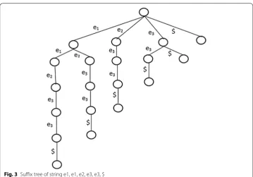
Example Let us assume an alphabet set

= {e1,e2,e3,e4} and a string X=e1,e1,e2,e3,e3, $. All the suffixes are as shown in Table 2 and resulting suffix tree is as shown in Fig. 3.

Generalized suffix tree was initially proposed in [31]. Unlike other suffix trees which process one long sequence. The generalized suffix tree is constructed from a set of string. This work focuses on the construction of generalized suffix tree through distrib-uted computing leveraging map-reduce processing framework. As part of processing frequency of occurrence of each suffix is taken care and probability of nodes are com-puted. This tree is known as probabilistic generalized suffix tree (PGST).

Proposed approach

Two phase probabilistic generalized suffix tree (PGST) construction basics

A suffix tree constructed from a collection of strings is known as a generalized suffix tree. Given is a set of strings S= {S1,S2. . ...Sn}, where Si∈∀1≤i≤n. Each Si is appended with symbol $∈/

so that none of the suffix is a substring of any other suffix. This ensures each suffix creates a leaf in the tree. We propose a two-step process to com-pute generalized suffix tree from S.

1. First phase computes all suffixes.

2. Second phase constructs tree from suffixes computed earlier.

Fig. 2 User trip mapped to road network

Table 2 All suffixes for e₁, e₁, e₂, e₃, e₃, $

i xi Suffix

1 x₁ e1,e1,e2,e3,e3, $

2 x₂ e1,e2,e3,e3, $

3 x₃ e₂,e₃,e₃, $

4 x₄ e₃,e₃, $

5 x₅ e₃, $

Two-phase implementation is very intuitive for implementation under distributed map reduce framework. First phase is implemented by mapper module and second phase is implemented by reducer. Process is described in next section. In the first phase, suffixes for each Si ∈S are calculated and put in a map where key is suffix itself and value is number of time it occurs in S. Processing is as described in Algorithm 1 below.

The process is demonstrated through the example below. Following four sequences we take for demonstration and is used as running example in all next sections. S0=e1,e2,e3,e4, $S1=e1,e2,e3,e4, $S2=e1,e5,e3,e4, $S3=e3,e4, $. Suffix set is cal-culated for each sequence. Map with each suffix and their occurrence count computed by Algorithm  1 is summarized in Table 3. Combined length of all the sequences is n=n

i=1|Si|. For a given sequence Si number of suffixes nd can be computed in O|Si|. Hence suffixes of all sequences can be calculated in On

In the second phase, we start with the empty tree and insert the suffixes from the map in sequence. If any suffix sequence is unique makes a completely new branch. If the par-tial matching sequence is already found in the tree then till the match is found frequen-cies are summed up and for the unique portion, a new branch is formed. Algorithm II explains the process. Figure 4 shows result of inserting suffix e1,e2,e3,e4, $ in empty tree. Next we insert a partial overlapping suffix e1,e5,e3,e4, $. Figure 6 represents final suffix

tree generated.

Table 3 Suffixes and their occurrence count

i xi Suffix Count

1 x1 e1,e2,e3,e4, $ 2

2 x2 e2,e3,e4, $ 2

3 x3 e3,e4, $ 4

4 x4 e4, $ 4

5 x5 $ 4

6 x₆ e1,e5,e3,e4, $ 1

7 x7 e5,e3,e4, $ 1

At any point of time height of the tree is h≤max(|Si|∀1≤i≤n) is the length of long-est suffix. Total number of suffixes to be inserted in tree is n=n

i=1|Si|. Each insertion starts with root and can go till leaf i.e. total nos to be traversed can be up to h. So com-plexity of this phase is O(nh)≤O(n2) which dominates overall complexity.

Distributed construction of PGST tree

Map-reduce is a programming technique for processing large data sets with a parallel, distributed algorithm on a cluster. Map-reduce works in two phases: the Map phase and the reduce phase. Each phase has 〈key, value〉 pairs as input and output. Mapper is a function that iterates over input data set and transforms data into key-value pair [33]. In order to achieve parallelism, framework library splits the huge input data set into multi-ple chunks of typically 16–64 MB based on configuration provided [34]. Then multiple copies of mapper module are spawned over different nodes in the cluster each of which processes a chunk of the huge input data. Once the mappers finish computing key-value pairs of the input data, then it’s the responsibility of Map-Reduce framework to group all intermediate values associated with the same intermediate key and passes them to reducer function. Reducer is a function which is triggered after all the mappers are fin-ished and intermediate (key, value) pairs are aggregated. Reducer function iterates over the key set and for a set of values associated with each key performs the reduction possi-bly smaller set of values [35]. In summary, Reducer merges all intermediate values asso-ciated with the same key. Map reduce runs on a huge cluster composed of commodity computing nodes and is highly scalable. This kind of scalability is known as horizontal scalability.

Two phase suffix tree construction technique described in the previous section is executed under map reduce framework to achieve horizontal scalability. The motive of designing two-phase algorithm for suffix tree construction was that it makes technique easily portable to map reduce framework. The first phase where contexts are calculated is executed by mapper module and the second phase which does construction of suffix tree from context strings is executed by reducer module.

The set of string sequences S= {S1,S2. . ..Sn} is partitioned according to the num-ber of computing nodes in the cluster. If the numnum-ber of the nodes in the cluster are, then the number of partitions created are |S|

k. For each of the partition of strings, a mapper module is triggered. Mapper locally operates on set a of sequences assigned to it and output is the map of suffixes a keys and values as frequency of their occur-rence similar to Algorithm I above. For demonstration we take S contains following four strings S1=e1,e2,e3,e4, $S2=e3,e4, $S3=e1,e2,e3,e4, $S4=e1,e5,e3,e4, $. If k = 2 then two partitions are created, Partition I:S1=e1,e2,e3,e4, $S2=e3,e4, $ and

Mapper function iterates over input sequence and prepares intermediate 〈key, value〉 pairs. Intermediate results are buffered in memory mapper worker and periodically writ-ten to distributed file system.

The intermediate output 〈suffixi, counti〉 from each mapper is grouped appropriately by Map-Reduce framework and then passed onto Reducer for further processing. It ensures the keys are unique. If multiple copies of the same key are received then their values are consolidated in a list before sending it to Reducer. The result of the consolida-tion of the output of mappers in Tables 4 and 5 is as shown in Table 6.

Reducer receives key and associated list of values 〈zi, 〈value_list〉〉. Reducer function processes this 〈zi, 〈value_list〉〉 to compute the sum of all frequencies corresponding to each key before inserting in the tree. Key and sum of values in the associated list is as shown in Table 7. Diagrammatic representation of Tables 4, 5, 6 and 7 is given in Fig. 5 for better understanding.

Table 4 All suffixes and their counts computed by mapper-x

i xi Suffix Count

1 x1 e1, e2, e3, e4, $ 1

2 x2 e2, e3, e4, $ 1

3 x3 e3, e4, $ 2

4 x4 e4, $ 2

5 x5 $ 2

Table 5 All suffix and their frequency count computed by mapper-y

j yj Suffix Count

1 y1 e1, e2, e3, e4, $ 1

2 y2 e2, e3, e4, $ 1

3 y3 e3, e4, $ 2

4 y₄ e4, $ 2

5 y5 $ 2

6 y6 e1, e5, e3, e4, $ 1

The process starts from an empty tree. As soon as for a key, the sum of value_list is computed, key as the string is inserted in PGST along with frequency count. Keys as context string is iteratively inserted into this tree. Since we add frequencies during each insertion overall frequency for each node remains same as when computed on a single node. For example, when computed on single node suffix e3,e4, $ has frequency 4 on each corresponding node of the tree. In reducer module for the same suffix in mapper-x and mapper-y frequency is 2 in each. Reducer will insert this suffimapper-x twice and hence for this suffix frequency count will be 4. The process is implemented in reducer func-tion and is as described in Algorithm IV below. Resultant tree is same as constructed by Algorithm II on single machine and shown in Fig. 6.

Table 6 Result of merging of intermediate key/value pairs by Map-Reduce framework

i zj Key (k) Values (v) 〈K, 〈value_list〉〉

1 z1 e1,e2,e3,e4, $ 1, 1 〈e1,e2,e3,e4, $, 〈1, 1〉〉

2 z2 e2,e3,e4, $ 1, 1 〈e2,e3,e4, $, 〈1, 1〉〉

3 z3 e3, e4, $ 2, 2 〈e3,e4, $, 〈2, 2〉〉

4 z4 e4, $ 2, 2 〈e4, $, 〈2, 2〉〉

5 z5 $ 2, 2 〈$, 〈2, 2〉〉

6 z6 e1,e5,e3,e4, $ 1, 0 〈e1,e5,e3,e4, $, 〈1, 0〉〉 7 z7 e5,e3,e4, $ 1, 0 〈e5,e3,e4, $, 〈1, 0〉〉

Table 7 Computation of sum of value_list associated with keys by reducer function

i zj 〈K, 〈value_list〉〉 〈K, sum (values)〉

1 z1 〈e1,e2,e3,e4, $, 〈1, 1〉〉 〈e1,e2,e3,e4, $, 〈2〉〉

2 z2 〈e2,e3,e4, $, 〈1, 1〉〉 〈e2,e3,e4, $, 〈2〉〉 3 z3 〈e3,e4, $, 〈2, 2〉〉 〈e3,e4, $, 〈4〉〉

4 z4 〈e4, $, 〈2, 2〉〉 〈e4, $, 〈4〉〉

5 z5 〈$, 〈2, 2〉〉 〈$, 〈4〉〉

6 z₆ 〈e₁,e₅,e₃,e₄, $, 〈1, 0〉〉 〈e₁,e₅,e₃,e₄, $, 〈1〉〉 7 z7 〈e5,e3,e4, $, 〈1, 0〉〉 〈e5,e3,e4, $, 〈1〉〉

Route prediction

Route prediction related work and literature

Approaches for route prediction algorithms found in literature can be categorized into two groups: spatiotemporal correlation and statistical methods. Authors in [3] presented a Spatio-temporal correlation based route prediction technique. The trip similarity is established and clustered using hierarchical agglomerative clustering approach. Two route prediction approaches are proposed. In the first approach, the closest match to a partial trajectory is computed on traversal of each new edge and next link is forecasted as next edge from the closest matching historical trip.

In the second approach, threshold match algorithm returns route and confidence meas-ure provided a partial trajectory traveled so far. Horizontal scalability aspect is not taken care. Authors in [36] proposed urban traffic amount prediction for route guidance systems. Prediction is based on spatiotemporal correlation of the road network. It does not make use of historical travel pattern of traffic but is purely based on current state of the system.

Laasonen [37] proposed route prediction system using cellular data. The geographical area is divided into cellular regions. The mobility of user is defined in terms of move-ment between cellular regions. Mobility vector is composed of Ids of cellular regions. User location, cellular region, is predicted based on historical travel pattern of the user

between the cellular regions. It does not make use of digitized road networks. None of these algorithms address scalability issues.

Statistical approaches are based on Variations of Markov model (VMM). Vari-ous VMM approaches like context tree weighting (CTW), prediction by partial match (PPM), probabilistic suffix tree (PST) and Lempel–Ziv (LZ78) algorithms for prediction of sequences based on partial sequences are well explored [10]. Sequence predictions were evaluated for protein sequences, text data, music files etc. Route prediction is not covered by this work. Additionally, scalability issues are not addressed. Work presented in [38] summarized various statistical approaches for route prediction: Markov model (MM), hidden Markov model (HMM) and variable order Markov model (VMM). In the proposed approach, the issue of horizontal scalability is addressed.

Route prediction using probabilistic suffix tree (PST)

Problem statement Given a partial trajectory traveled

x_t0,y_t0,t0

,

x_t1,y_t1,t1

. . .xtn,ytn,tn, predict the next link σ ∈ E on road network based on historical travel pattern.

Given a partial trajectory, first step is to map the trajectory on road net-work using map matching (as described in earlier) f(

x_t0,y_t0,t0

,

x_t1,y_t1,t1

. . .

xtn,y_tn,tn₎→e_i,e_{i+1. . .}e_i+k where e_i,e_{i+1. . .}e_i+k∈E.

As defined above, f is map matching function which maps ordered time stamped sequence of location data traces to edges of the road network. Hence route prediction is a function R that takes input trajectory ei,ei+1. . .ei+k and predicts next link σ on the road represented as R

ei,ei+1. . .ei+k

→σ∈E.

Each trip/trajectory can be thought of as Markov chain such that next outcome σ depends only on present state.

where p calculates conditional probability. Markov chain is K-order if

p(σ|e_ie_i+1. . .e_i+n)=p(σ|e_i+ke_i+k+1...e_i+n).

Probabilistic suffix tree constructs all Markov sequences (1:k) road segment sequence to predict next road segment. In this case, k is the length of longest trip. Length of long-est branch in the tree and hence height of the tree is O (k).

Suffix tree model learns from historical travel pattern. Suffix tree constructed in sec-tion IV is a variable order Markov model and is used for route predicsec-tion. It is built assuming that the trip eiei+1. . .ei+n is a Markov chain. Possible events (σ) in route pre-diction is set of edges E of graph G(V,E). Probability distribution with respect to root of the tree is as shown in Fig. 7.

Following scenarios demonstrates the route prediction function R

Scenario I: Input trajectory is ε. This case represents when input trajectory is

empty and none of the edges of the road network graph is yet tra-versed. According to the suffix tree candidate edges for travel are

{e1,e2,e3,e4,e5}. Probabilities for each candidate is as: p(e1|ǫ)= 3

10, p(e2|ǫ)= 2

10, p(e3|ǫ)= 104, p(e5|ǫ)= 101, Hence R(ǫ)→e3 means e3 is

Scenario II: Input trajectory is {e2}. This case is when input trajectory is of length

1. According to the suffix tree only candidate edges for travel is {e3} .

Probability for candidate is p(e3|e2)= 2₂=1. Hence R(e2)→e3

means e3 is predicted edge

Scenario III: Input trajectory is {e1}. According to the suffix tree candidate edges

for travel are {e2,e5}. Probabilities for each candidate are p(e2|e1)= 2₃,

p(e5|e1)= 1₃. Hence R(e1)→e2 means e2 is predicted edge

Scenario IV: Input trajectory is {e1,e5}. According to the suffix tree candidate edge

for travel is {e3}. Probabilities for candidate is p(e3|e1,e5)=1. Hence

R(e1,e5)→e3. means e₃ is predicted edge

Scenario V: Input trajectory is {e3,e4}. According to the suffix tree candidate edge

for travel is ∅. Hence R(e1,e5)→ǫ means prediction not possible. It

can happen in two scenarios:

a. Traveler has reached its destination.

b. Traveler has taken a new route which model has not observed earlier.

Scenario VI: All of the above cases focused on predicting one hop next edge. The

same model can be used to predict an end to end path as well. Input

trajectory is ǫ. As in case I, next edge selected is e₃. From e₃ next

probable edge is e2 and so on.

Implementation and evaluation

The implementation of the proposed system requires two kinds of data:

1. Map data and 2. GPS location traces.

Map data‑spatial road network data

Geographical spatial data is sourced from Open street maps (OSM), an open source map database. Open street maps create and provides free geographic data such as street maps and are published under an open content license, with the intention of promot-ing the free use and re-distribution of the data (both commercial and non-commercial)

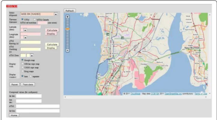
[39]. Like Google maps, it provides the maps as the images and also the spatial and non-spatial data in the form of shape files or XML files. Maps can be zoomed and viewed up to different levels. OSM too provides the APIs to access map images through HTTP request. From this interface, an area can be zoomed in and can be selected to export to the local client as an image file (GIF, PNG or JPEG) or as a .osm file in XML format. Through OSM interface various spatial data can be downloaded—Centerline of Roads, Polygons of Buildings, State and International boundaries as lines, Water bodies poly-gons etc. Data of the whole world, country wise, state wise are available to download. Osm2pgsql is a utility with PostgreSQL that can be used to load the content of the .osm file to PostgreSQL database. For each type of the feature like road lines, polygons etc., there is a separate file. OSM interface integrated into our application is shown below in Fig. 8.

It is required to load each of these files separately into the database. The OSM file con-taining all the data of the whole world is about 15 GB in compressed form. An applica-tion is built for data visualizaapplica-tion. The applicaapplica-tion is web based and is developed using JAVA web technologies with facilities for users to Interact with rich user interfaces. The result of queries is the Map Layers which is a combination of.

• Open layers (maps formed by fetching data from data base) and

• Base map images (Google Map Images or OSM Map Images can be used).

Open Layers are rendered using Geoserver. Geoserver is again an open source soft-ware. It uses Web Map Service (WMS) standard to connect to Spatial DB (in this case PostGIS) and render the spatial features stored in the databases. Geoserver works through HTTP service and can be easily embedded in web pages. Open street maps (OSM) or Google Map Images are used as base map image layer. In this research work, visualization of data is done by keeping OSM maps as base layer and Road and poly-gon layers created as an open layer in Geoserver. Geoserver takes the data from PostGIS

database. Figure 9 shows the setup of the module implemented for visualization of spa-tial data. Figures 10 and 11 below are a snapshot of the road network and polygon data visualization from application respectively.

GPS location traces data

For experiments, GPS location traces data is used that is collected and distributed by Microsoft under project Geolife. This data was collected over a span of around 4 years and mainly from Beijing area of China [40]. This data is a continuous log of time-stamped latitude/longitude representing the position of the user with respect to time. This data was decomposed into more granular segments called trips as described in preceding sections. Data collected by 178 users has around 17,672 trajectories cover-ing around 1.25 million kilometers of distance. Data was collected uscover-ing GPS device with data capturing frequency of 1–5 s. Data was collected from the user while carrying

Fig. 9 Application for spatial data visualization

different activities like the transition between office and home, sightseeing, dining etc. Dataset is used in many recent researches related to map matching, user activity recog-nition, mobility pattern mining, location recommendation etc. A sample data collected through GPS and rendered over Open street map (OSM) is shown below in Fig. 12.

For horizontally scalability, data from PostGIS was imported in HDFS based data store Hbase. Road segments were further indexed in a grid indexing. Each grid contains all the road segments spatially belonging to minimum bounding rectangle (MBR) of the grid. Union of all the grid is necessarily all the MBR of the original map and contains all the roads of the network under consideration. Replication factor affects time complexity. If it’s too low then lots of time goes into network latency for data transfer to the computing node. To achieve better results we kept replication factor equal to the number of com-pute nodes. So that data is available on all computation nodes and we don’t spend too much time in data transfer. The experiment was performed over cluster containing six compute machines (five workers and one master node). Each node has a 64-bit proces-sor with 8 GB main memory. Increasing number of trips give a better model and hence

Fig. 11 Polygon features rendered over Open Street Maps

gives a better performance. Secondly, closer the user is, to the destination more data points are available for prediction and explains better prediction. Experimental results showing prediction in accuracy in terms of distance traveled by user and percentage of trip completed by user is shown in Figs. 13 and 14 respectively. Accuracy of around 95% was achieved. Processing time on single machine is shown in Fig. 15 and on cluster is shown in Fig. 16.

Fig. 13 Prediction accuracy in terms of miles of trip completed

Future work

Proposed end to end route prediction application is based on probabilistic generalized suffix tree (PGST) model. Alternative statistical modeling approaches exist in literature and applied in different fields of study like text mining, speech recognition, bioinformat-ics, string matching etc. To name a few such methods are CTW (context tree weighting), PPM (prediction by partial match) and LZ78 etc. The problem with them is horizon-tal scalability is not resolved to best of our knowledge. These alternatives can be tried

Fig. 15 Processing time on single machine

out and see whether they have potential to further enhance accuracy and computational efficiency. Other than statistical are approaches like clustering, association rule mining, neural networks etc. Very less research is done on their applicability in the field of route prediction as well their horizontal scalable versions are still a challenge.

Conclusion

In this research work, the focus was on building a horizontally scalable end to end appli-cation for route prediction appliappli-cation. Raw GPS traces are converted to trips composed of edges of the digitized road network by map matching. A Map-reduce based parallel version of map matching is implemented to overcome huge computational time required during this step. Hbase is used for storage and map-reduce framework for performing map matching. This reduces both—storage requirement as well as the computational time. Next phase is model construction for which probabilistic generalized suffix tree (PGST) is leveraged. In this work, PGST is used for route prediction. Challenging part is scalability of PGST construction. The map-reduce framework is employed to achieve horizontal scalability. A two-step process is followed, which is very intuitive to imple-mentation in map-reduce framework. The end-to-end horizontally scalable application is designed and implemented for route prediction. Data visualization is also equally important and hence implemented using an open source technology based spatial data visualization tool integrated with the application. All tools and technologies used are open source. Experiments are performed on real datasets and snapshots are taken from real data.

Authors’ contributions

VST and AA discussed the idea of PST and PGST with respect to route prediction and its implementation aspects. VST has implemented the idea and contributed towards the first draft of the paper under the guidance of AA. AA thoroughly proofread the manuscript and made all vital corrections. Both authors read and approved the final manuscript. Authors’ information

Vishnu Shankar Tiwari is a post graduate (Master of Technology- M. Tech.) in Computer Engineering from Department of Computer Engineering, Indian Institute of Technology (IIT)-Bombay, Mumbai, India. Also, holds M. Tech. (Computer Applications) from YMCA University of Science and Technology, India and Master of Computer Application (MCA) from Maharshi Dayanand University, India. Working in software industry for more than 8 years.

Arti Arya is Head of Department (HOD) and Professor at Department of Computer Application, PES Institute of Tech-nology, Bangalore South Campus. She holds Ph. D in Computer Science from Faculty of Technology and Engineering, Maharshi Dayanand University, India. She has M. Tech in Computer Science from Allahabad Agricultural Institute, Master of Science (Mathematics) and Bachelor of Science (Mathematics) from Delhi University. Her areas of interests are Spatial Data Mining, Knowledge based systems, Machine Learning, Artificial Intelligence, Data Analysis. She has approx. 17 years of teaching experience (of which 10 years of research) at Undergraduate and Post Graduate level. She is Senior Member IEEE, Life Member CSI and Life Member IAENG.

Acknowledgements

We thank Geospatial Information Science and Engineering (GISE) Lab, Indian Institute of Technology, IIT-Bombay, India for carrying out some initial part of the work at their lab. We would also like to thank anonymous reviewers, whom reviews helped us to bring this manuscript to the current form.

Competing interests

The authors declare that they have no competing interests. Availability of data and materials

All data and material used is open source. Majorly, GPS data points are from GPS trajectory dataset collected in (Microsoft Research Asia) Geolife project. Dataset is made available for research from 2012 by Microsoft Research (https://geotime. com/general/geolife-project/). Map data used is from Open street map (OSM) which is an open project (http://www. openstreetmap.org).

Consent for publication

Ethics approval and consent to participate

This is author’s own personal research work. Authors self-approve ethical approval and provide consent for participation. Funding

This work is purely authors own work and authors own funding required for publishing of this research work.

Publisher’s Note

Springer Nature remains neutral with regard to jurisdictional claims in published maps and institutional affiliations.

Received: 25 May 2017 Accepted: 9 July 2017

References

1. Tiwari VS, Arya A, Chaturvedi SS. Route prediction using trip observations and map matching. In: Advance comput-ing conference (IACC), 2013 IEEE 3rd international, 22–23 Feb 2013, p. 583–7.

2. Tiwari VS, Arya A, Chaturvedi S. Framework for horizontal scaling of map matching using map-reduce. In: IEEE, 13th international conference on information technology, ICIT 2014, 22–24 Dec 2014. http://www.icit2014.in/.

3. Froehlich J, Krumm J. Route prediction from trip observations. In: Society of automotive engineers (SAE) 2008 World Congress, Apr 2008, Paper 2008-01-0201.

4. Zhou J, Golledge R. A three-step general map matching method in the gis environment: travel/transportation study perspective. Int J Geogr Inf Syst. 2006;8(3):243–60.

5. Greenfeld JS. Matching GPS observations to locations on a digital map. In: Proceedings of the 81st annual meeting of the transportation research board, Washington DC; 2002.

6. Meng Y, Chen W, Chen Y, Chao JCH. A simplified map-matching algorithm for in-vehicle navigation unit. Research report, Department of Land Surveying and Geoinformatics, Hong Kong Polytechnic University; 2003.

7. Li J, Fu M. Research on route planning and map-matching in-vehicle GPS/dead reckoning/electronic map inte-grated navigation system. In: IEEE proceedings on intelligent transportation systems; 2003, 2, p. 1639–43. 8. Bernstein D, Kornhauser A. An introduction to map matching for personal navigation assistants, technical report.

NewJersey TIDE Center Technical Report, 1996.

9. Li Y, Huang Q, Kerber M, Zhang L, Guibas L. Large-scale joint map matching of GPS traces. In: Accepted for the 21st ACM SIGSPATIAL international conference on advances in geographic information systems (ACM SIGSPATIAL GIS 2013).

10. Begleiter R, El-Yaniv R, Yona G. On prediction using variable order Markov models. J Artif Intell Res. 2004;22:385–421. 11. Comin M, Farreras M. Efficient parallel construction of suffix trees for genomes larger than main memory. In:

EuroMPI’13, Proceedings of the 20th European MPI user’s group meeting; 2013.

12. Bieganski P, Riedl J, Carlis J, Retzel EF. Generalized suffix trees for biological sequence data. In: Proceedings of the twenty-seventh Hawaii international conference on biotechnology computing. p. 35–44, 1994.

13. Mansour E, Allam A, Skiadopoulos S, Kalnis P. ERA: efficient serial and parallel suffix tree construction for very long strings. Proc VLDB Endow (PVLDB). 2011;5(1):49–60.

14. McCreight EM. A space-economical suffix tree construction algorithm. J ACM. 1976;23(2):262–72. 15. Ukkonen E. On-line construction of suffix trees. Algorithmica. 1995;14(3):249–60.

16. Farach-Colton M, Ferragina P, Muthukrishnan S. On the sorting complexity of suffix tree construction. J ACM. 2000;47(6):987–1011.

17. Hunt E, Atkinson MP, Irving RW. A database index to large biological sequences. In: VLDB; 2001, p. 139–48. 18. Bedathur SJ, Haritsa JR. Engineering a fast online persistent suffix tree construction. In: ICDE; 2004, p. 720–31. 19. Cheung C-F, Yu JX, Lu H. Constructing suffix tree for gigabyte sequences with megabyte memory. IEEE Trans Knowl

Data Eng. 2005;17(1):90–105.

20. Hariharan R. Optimal parallel suffix tree construction. In: STOC; 1994, p. 290–9.

21. Landau GM, Schieber B, Vishkin U. Parallel construction of a suffix tree (extended abstract). In: ICALP; 1987, p. 314–25. 22. Satish UC, Kondikoppa P, Park S, Patil M, Shah R. Mapreduce based parallel suffix tree construction for human

genome. In: 20th IEEE international conference on parallel and distributed systems ICPADS 2014 Hsinchu Taiwan, 2014, 201, p. 664–70.

23. Ghoting A, Makarychev K. Indexing genomic sequences on the IBM blue gene. In: Proceedings of conference on high-performance computing networking, storage and analysis (SC); 2009, p. 1–11.

24. Marchal F, Hackney J, Axhausen KW. Efficient map-matching of large GPS data sets—Tests on a speed monitoring experiment in Zurich. Arbeitsbericht Verkehrs- und Raumplanung, Institut f ̈ur Verkehrsplanung und Transportsys-teme, ETH Zürich, Zürich; 2004.

25. Quddus MA. High integrity Map-matching algorithms for advanced transport telematics applications, Ph.D. Thesis. UK: Centre for Transport Studies, Imperial College London; 2006.

26. Quddus MA, Noland RB, Ochieng WY. A high accuracy fuzzy logic based map matching algorithm for road trans-port. J Intell Transp Syst. 2006;10(3):103–15.

27. Weiner P. Linear pattern matching algorithms. In: SWAT; 1973, p. 1–11.

28. Tata S, Hankins RA, Patel JM. Practical suffix tree construction. In: Proceedings of VLDB; 2004, p. 36–47. 29. Tian Y, Tata S, Hankins RA, Patel JM. Practical methods for constructing suffix trees. VLDB J. 2005;14(3):281–99. 30. Phoophakdee B, Zaki MJ. Genome-scale disk-based suffix tree indexing. In: Proceedings of the 2007 ACM SIGMOD

31. Barsky M, Stege U, Thomo A. Suffix trees for inputs larger than main memory. Inf Syst. 2011;36(3):644–54. 32. Erciyes K. Distributed and sequential algorithms for bioinformatics. Cham: Springer International Publishing; 2015. 33. Dean J, Ghemawat S. MapReduce: simplified data processing on large clusters. In: Proceedings of the 6th

confer-ence on symposium on opearting systems design & implementation, 06–08 Dec 2004, San Francisco, CA, p. 10. 34. Chang F, Dean J, Ghemawat S, Hsieh WC, Wallach DA, Burrows M, Chandra T, Fikes A, Gruber RE.

Bigta-ble: a distributed storage system for structured data. ACM Trans Comput Syst (TOCS). 2008;26(2):1–26. doi:10.1145/1365815.1365816.

35. Lammel R. Google’s MapReduce programming model—Revisited. Sci Comput Program. 2008;70:1–30.

36. Liang Z, Wakahara Y. Real-time urban traffic amount prediction models for dynamic route guidance systems. J Wirel Commun Netw. 2014;2014:85.

37. Laasonen K. Route prediction from cellular data. In: Workshop on context-awareness for proactive systems (CAPS); 2005.

38. Nagraj U, Kadam N. Vehicular route prediction in city environment based on statistical models. J Eng Res Appl. 2013;3(5):701–4.

39. https://www.openstreetmap.org.