O R I G I N A L A R T I C L E
Open Access
Marriage markets as explanation for why
heavier people work more hours
Shoshana Grossbard
1,2,3*and Sankar Mukhopadhyay
4,2* Correspondence: shosh@mail.sdsu.edu
1Department of Economics, San
Diego State University, 5500 Campanile Drive, San Diego, CA 92182, USA
2IZA, Bonn, Germany
Full list of author information is available at the end of the article
Abstract
Is BMI related to hours of work through marriage market mechanisms? We
empirically explore this issue using data from the NLSY79 and NLSY97 and a number of estimation strategies (including OLS, IV, and sibling FE). Our IV estimates (with same-sex sibling’s BMI as an instrument and a large set of controls including wage) suggest that a one-unit increase in BMI leads to an almost 2% increase in White married women’s hours of work. However, BMI is not associated with hours of work of married men. We also find that a one-unit increase in BMI leads to a 1.4% increase in White single women’s hours of work, suggesting that single women may expect future in-marriage transfers that vary by body weight. We show that the positive association between BMI and hours of work of White single women increases with self-assessed probability of future marriage and varies with expected cumulative spousal income. Comparisons between the association between BMI and hours of work for White and Black married women suggest a possible racial gap in intra-marriage transfers from husbands to wives.
Keywords:Obesity, Labor supply, Marriage, Marriage market, Gender, Race, Intra-household bargaining, Personal finances
JEL Classification:J22, I12, J12
1 Introduction
Obesity is a major problem in the industrialized world, including the US. Its health and health cost consequences have been well documented, e.g., in Strum (2002) and Cawley and Meyerhoefer (2012). In addition, higher body weight may have negative social and economic consequences. Several studies (Register and Williams 1990; Averett and Koren-man 1996; Pagan and Davila 1997; Cawley 2004; Atella et al. 2008; Johar and Katayama 2012; Cawley and Meyerhoefer 2012; Sabia and Rees 2012; Larose et al. 2016 among others) have found an inverse relationship between women’s earnings and their body weight. There is a related but smaller literature that explores the effects of BMI on em-ployment status. Lindeboom et al. (2010) do not find any significant effect of obesity on employment in the UK. Morris (2007) on the other hand finds that obese women are less likely to participate in the labor market in the UK. Two experimental studies, Rooth (2009) and Reichert (2015), find a negative effect of BMI on employment. Caliendo and Gehrsitz (2016) provide semiparametric estimates for the relationship between BMI and employment and find evidence of non-linearity.
Furthermore, body weight has negative consequences for a number of outcomes related to couple formation. It reduces (1) women’s dating and matching opportunities (Lemenni-cier 1988, Hitsch et al. 2010, Vaillant and Wolff 2011; Chiappori 1992), (2) their likelihood of cohabitation and marriage (Mukhopadhyay 2008) but not in a linear way (Malcolm and Kaya 2016), and (3) a wife’s relative influence on how the couple’s resources are internally distributed (Oreffice and Quintana-Domeque 2012). Singles with higher BMI may expect less from marriage. For instance, Vaillant and Wolff (2011) show that French obese women are less likely to expect men to be tall and charming and are more willing to accept a violent mate. Obese women are also less likely to be married to men with higher income and edu-cation (Oreffice and Quintana-Domeque 2010).
Our research focus is on the impact of BMI on market hours of work and on whether this impact operates via mechanisms related to marriage markets, such as intra-marriage financial transfers, bargaining about access to consumption, or, in the case of singles, marriage expectations or predicted spousal income and access to household in-come. A pioneering study on this topic is Oreffice and Quintana-Domeque (2012) (hereafter OQD) who found that married White men and women who are heavy rela-tive to their spouse work more hours. They interpreted this finding in terms of a posi-tive effect of thinness on individual access to a couple’s resources, assuming that thinness is valued in marriage markets and therefore increases an individual’s intra-marriage bargaining power In contrast, they did not find any relation between BMI and hours of work for single White women.
Other previous research has hypothesized that factors related to value in marriage mar-kets could possibly affect hours of work or labor-force participation. Heer and Grossbard-Shechtman (1981) are the first to have examined empirically how one such factor, the sex ratio defined as the ratio of men to women in a marriage market, helps explain changes in women’s labor-force participation over time.1The potential impact of individual character-istics on women’s labor-force participation via their effect on marriage markets was first studied by Grossbard-Shechtman and Neuman (1988), using relative age and ethnicity as individual characteristics.2Furthermore, Hersch (2013) found that married women who graduated from elite colleges are more likely to drop out of the labor force after having a child. One of her interpretations for that finding is that the quality of a college education is positively related to marriage market outcomes, including husband’s earning power.
We use data from two cohorts of the National Longitudinal Survey of Youth: the 1979 cohort and the 1997 cohort (the NLSY79 and the NLSY97, respectively, from now on) and examine the association between BMI and hours of work for men and women who are ei-ther married to their first spouse or are unmarried. Since NLSY interviews all eligible youths in an eligible household, we know the relevant information for the siblings of re-spondents as well. This allows us to use two strategies to establish causality. We use sibling fixed effects (FE) and instrumental variable (IV) regression with same-sex sibling BMI as an instrument to establish causality. Our data also includes relatively large samples of Blacks and Hispanics, thus allowing us to compare our findings for various ethnic groups. However, we do not have data on spouse’s BMI, which prevents us from testing some of OQD’s predictions regarding effects of a spouse’s relative weight on hours worked.
IV estimates suggest that a one-unit increase in BMI leads to a 1.4% (2.0%) increase in hours worked among White single (married) women.
What is unique about our paper is the variety of ways by which we attempt to uncover the possible mechanisms that can explain the effects of BMI on hours of work, with a focus on explanations related to the functioning of marriage markets. First, we estimate the effect of BMI on hours worked with and without wage, in order to examine the degree to which the effect of BMI on hours of work derive from the effect of BMI on wage. We find consistent evidence indicating that BMI increases hours of work for White (both single and married) women regardless of whether wage is controlled for. Given that we obtain similar results using both sibling fixed effects and IV regressions, these associations may represent causal effect of BMI on hours of work. Our results suggest that the positive association cannot be explained via wage effects and opens the door to explanations based on marriage market effects.
Then we use the richness of the NLSY data to explore a plethora of possible mecha-nisms. The NLSY includes information on expectations about marriage, health status, availability of employer-provided health insurance, and a number of spousal characteris-tics, including age, education, and annual income. We use this information to explore mechanisms behind the positive association between BMI and hours of work. For ex-ample, we show that, while high BMI is associated with lower spousal income, for White married women, the association between BMI and hours of work remains significant even after controlling for spousal characteristics, including income.
This suggests that high-BMI married women have less access to spousal income, con-ditional on their husband’s income. We also explore whether marriage market mecha-nisms lie behind the relationship between BMI and hours of work in single women. For example, we show that the positive association between BMI and hours of work in White single women increases with self-assessed probability of future marriage. In addition, for single women, after including expected cumulative spousal income, we find a smaller positive association between BMI and hours of work.
To the extent that our findings suggest that a positive association between body weight and hours of work is related to a negative association between weight and intra-marital transfers, our interpretation is compatible with that of OQD. They conclude that individ-uals with high BMI (relative to that of their spouse) may obtain lower Pareto weights in their marriage. Our results are also consistent with the explanation that thinner women (married or not) are in higher demand in marriage markets, relative to their counterparts who weigh more. The market model of marriage based on Becker (1973) and Grossbard-Shechtman (1984) presented in Section 2 elaborates on this explanation. It also helps understand why we find more of a positive association between BMI and hours of work for White married women than for their Black or Hispanic counterparts and for women than for men.
eligible for employer-provided health insurance via more hours of work. We test these possibilities using data on health status and availability of employer-provided health insur-ance. Our results suggest that neither of these mechanisms explains the observed relation-ship between BMI and hours of work. Finally, we conduct a series of checks for robustness to reasonable changes in sample construction criteria, methods, and functional form assumptions. The results of these tests strengthen our conclusion that marriage market mechanisms may partly explain the positive associations between hours of work and body weight that we report in our data analysis.
This paper is organized as follows: Section 2 presents the conceptual framework, Sec-tion 3 describes the data and methods, SecSec-tion 4 presents the empirical results, and Section 5 concludes.
2 Conceptual framework
Hours of work could vary as a function of body weight due to mechanisms related to ei-ther marriage or labor markets or both. In this section, we first discuss how marriage mar-ket mechanisms could help explain a relationship between BMI and hours of work and then we discuss how labor market mechanisms could help explain such a relationship.
2.1 Marriage market mechanisms
Labor supply may be a function of body weight via the effect of body weight on two out-comes related to marriage markets. First, the literature reviewed in the previous section suggests that high-BMI people will be less likely to be married and they are less likely to be married to higher income spouses than people who are low-BMI. In heterosexual mar-riage markets, individuals with higher body weight may be less in demand on the part of members of the other sex and thus less likely to become part of a couple.
Second, lower demand in marriage markets may also lead to lower price. According to Becker (1973, 1981), to the extent that prices are established in multiple interrelated hedonic marriage markets, lower prices for married men or women may take the form of less access to consumption goods. This association between price in marriage market and access to consumption also follows from other theories of marriage such as McEl-roy and Horney (1981), Grossbard-Shechtman (1984), and Chiappori (1992). Becker (1973), McElroy and Horney (1981), and Chiappori (1992) assume that couples pool their resources in marriage and then decide on how to allocate the resources to individ-ual consumption. In contrast, Grossbard-Shechtman (1984) assumes that individindivid-uals keep control of their time and personal income whether married or not.3Consequently, prices in marriage markets may explainin-marriagefinancial transfers from one spouse to the other. The higher a person’s price in the marriage market, the higher the intra-household financial transfers they are likely to obtain from a spouse or the lower the financial transfers they are likely to make to a spouse (depending on whether they are a net financial beneficiary or a net financial contributor in the marriage). In turn, the more access a married person has to the spouse’s financial resources, the less they are likely to supply labor to the labor market (income effect).
both the spouse’s income and the spouse’s willingness to transfer some of that income in the marriage. Likewise, the price one pays for marrying a particular partner will be related to own income and own willingness to transfer some of that income to a spouse. Furthermore, single individuals planning to obtain a particular price in mar-riage may consider both a potential spouse’s income and their willingness to transfer as elements in their choice of mate. In the same vein, singles planning to pay a price in marriage will be influenced by their own income and prices in marriage markets.
High BMI is a factor related to relative demand in marriage markets. To the extent that they are in lower demand, high-BMI women (men) will command a lower price in marriage markets relative to that of low-BMI women (men) and consequently will be likely to obtain less personal access to consumption. Furthermore, they may either obtain fewer financial transfers from a spouse or may have to transfer more to a spouse once they are married. Consequently, we hypothesize thathigh-BMI married individuals will work more in the labor market than low-BMI people.
Spouses of high-BMI individuals are also likely to have a lower income than those married to low-BMI people. As for high-BMI people who are paying a price in mar-riage, they are likely to pay a higher price and may need more income compared to their low-BMI counterparts (Chiappori 1992, Oreffice and Quintana-Domeque 2012). Therefore, they may need to work more hours. High-BMI people may choose to marry individuals with attributes associated with lower prices (including higher weight, older age, and lower education) in order to avoid excessive financial obligations. This discus-sion suggests that BMI may also affect the hours of work of single people in the labor market. Hours of work in the labor market will vary with body weight regardless of marital status, to the extent that value in marriage markets affects both those who are already“employed”in marriage (or employing someone else) and those who are single and looking for a spouse. (This is similar to the idea that low wages affect the allocation of time of both the employed and the unemployed looking for a job.) In addition, to the extent that higher body weight has a negative effect on single individuals’ probabil-ity of marriage, this entails lower expected future access to spousal income as well. This is also likely to increase their hours of work prior to marriage. We thus hypothesize a positive effect of BMI on individual hours of work by both married and single individ-uals. In other words, effect of BMI would be similar in single and married women.
Body weight is likely to affect women’s hours of work more than men’s to the extent that women’s marriage prospects vary more with body weight than men’s (Mukhopad-hyay 2008) and that intra-marriage income transfers are more likely to flow from men to women than in the opposite direction. The latter gender difference is related to the observation that relative to married men, married women tend to earn less in the labor force and to do more household work, and to the idea that in-marriage income trans-fers may partially be compensations for household production work (Grossbard 2015).
with body weight for White women but not for Black women. To the extent that the pre-mium for being thin is higher in marriage markets for White women than in those for Black women, one expects more effects of body weight on intra-marriage transfers and thus on women’s hours of work for White women relative to those effects for Black women.
2.2 Labor market mechanisms
It is well-established (Cawley 2004 among others) that individuals (particularly White women) with higher BMI have lower wages compared to their lower-BMI counterparts. This can generate a substitution effect and an income effect. Therefore, theoretically, the effect of BMI on market hours of work, via lower market wages, is ambiguous. At the same time, most of the empirical literature suggests that women’s labor supply elas-ticity is positive (Blundell and MaCurdy 1999). In other words, a lower market wage (due to higher BMI) would induce women to work less. Therefore, this particular labor market mechanism and the marriage market mechanisms we mentioned above have different predicted effects regarding the association between BMI and hours worked.
There may be other ways that the labor market can affect the relationship between BMI and hours of work. If high-BMI workers have more health limitations, they may work less. However, if high-BMI workers anticipate a shorter working life, then they may work more during the early part of their life to compensate for an earlier exit from the labor force. An-other possible factor may be health insurance. To the extent high-BMI people value insur-ance more than low-BMI people do (presumably, because high-BMI people have or expect more health problems), they have more of an incentive to get health insurance and they may work more hours to qualify for an employer-provided insurance. Employers typically provide health insurance to full-time employees, and the Bureau of Labor Statistics defines full-time workers as someone working for more than 34 h per week. (However, the Affordable Care Act of 2009 defines a full-time employee as someone working more than 30 h per week.)
3 Data and methods 3.1 Data
We use data from two cohorts of National Longitudinal Survey of Youth (NLSY): the 1979 cohort (NLSY79) and the 1997 cohort (NLSY97). The NLSY79 started interviewing 12,686 respondents in 1979 when they were 14–22 years old. These individuals were interviewed every year until 1994 and after that on a biannual basis. The most recent wave (2014) in-cluded 9964 of the original respondents. The NLSY97 cohort started with 8984 respon-dents who were between the ages of 12 and 17 when they were first interviewed in 1997. Since then, they have been interviewed annually until 2011 and biannually thereafter. The most recent round of interviews (2013) included 7141 of the original respondents.
an interview, given that pregnancy can cause weight changes irrelevant to our analysis. We discard observations with weight below 70 lbs or above 400 lbs. We also discard observations with height below 4 ft or above 8 ft. We exclude data from marriages that end up in divorce, since our focus is on stable marriages. In our hours worked regres-sions, following the previous literature, we exclude respondents who worked 250 h or less in the previous year. If they are married, we exclude observations when the spouse of the respondent reported less than $5000 in annual income.
We use self-reported height and weight to compute BMI. In our data (both genders and all races combined), the 1st percentile of the BMI distribution is 17.2 and the 99th percentile is 45.5 (the 95th percentile is 39.7). These numbers are consistent with Sturm and Hattori (2013) who reported that 6.6% of US adults have a BMI of 40 or above. Then we Winsorize4the BMI distribution at 1% to reduce the effect of outliers. Our decision to Winsorize the BMI distribution (as opposed to dropping the extreme observations) is driven by two factors. First, a sizeable fraction (6.6%) of the US adult population have a BMI of 40 or above, and second, hours of work for respondents between a BMI of 30 and 40 and those with BMI above 40 are not significantly differ-ent (1865 h/year vs. 1896 h/year in our sample).5 We also Winsorize (at 1%) hourly wages of respondents to reduce the effects of outliers.
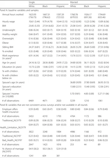
Table 1, panel A, contains the summary statistics for women for the variables used in this paper, separated by marital status and race.6The first three columns in this table are for single (never married and not cohabiting) women and the last three columns for married never-divorced women. Column 1 presents summary statistics for single White women. After imposing the abovementioned criteria, we have 6469 person-year observations for single White women. The average hours of work in this sample is 1624 h per year. Average real wage (in 2003 dollars) is $10.61. Average BMI is 23.85. Average age is 24.16 years, and average work experience (number of years with non-zero working hours) is 6.91 years. In other words, if an individual is enrolled in high school or college but worked at all (non-zero hours) during that year, then it still in-creases their work experience by one year. Single White females in our sample have 13.7 years of education, and about 35% are enrolled in school/college. About 7% of them have at least one child, and for 5%, the youngest child is below the age of six.
Summary statistics for Black and Hispanic single women are presented in columns 2 and 3 respectively. Single Black (Hispanic) women work on average about 1667 (1597) hours per year. The average wage for single Black (Hispanic) women is $9.79/h ($10.44/h). The average BMI for single Black (Hispanic) women is 27.5 (25.4). In both cases, the average BMI falls in the “overweight” category. Single Black and Hispanic women have less education and are more likely to have children relative to single White women.
Table 1 (panel B) presents the summary statistics and sample sizes for variables not used throughout the analysis. In NLSY, some questions were not asked in each round, or they are not consistent across surveys (NLSY79 vs. NLSY97). An example of the former is whether the employer of the respondent offers health insurance as a benefit. In reply, 59% (80%) of single (married) White women answered yes to this question. An example of the latter is whether a woman believes in traditional gender roles. The NLSY79 respondents were asked whether they agree or not with the following statement:“A woman's place is
Table 1Summary statistics for women
Single Married
White Black Hispanic White Black Hispanic
Panel A: baseline variables and samples
Annual hours worked 1623.95 (756.73)
1667.31 (796.62)
1597.39 (723.32)
1760.78 (679.53)
1926.17 (691.56)
1794.69 (655.46)
Hourly wage 10.61 (5.44) 9.79 (4.79) 10.44 (5.15) 14.33 (6.90) 13.23 (5.96) 13.09 (6.56)
BMI 23.85 (5.33) 27.54 (6.82) 25.41 (5.72) 25.08 (5.41) 28.58 (6.28) 27.45 (5.36)
Underweight 0.06 (0.24) 0.03 (0.17) 0.04 (0.19) 0.03 (0.18) 0.01 (0.12) 0.01 (0.10)
Healthy weight 0.66 (0.47) 0.41 (0.49) 0.54 (0.50) 0.57 (0.50) 0.29 (0.46) 0.36 (0.48)
Overweight 0.16 (0.36) 0.26 (0.44) 0.25 (0.43) 0.24 (0.42) 0.35 (0.48) 0.36 (0.48)
Obese 0.13 (0.33) 0.30 (0.46) 0.17 (0.38) 0.16 (0.37) 0.34 (0.47) 0.28 (0.45)
Sibling BMI 24.37 (4.81) 27.10 (6.21) 26.38 (5.63) 26.05 (5.29) 26.60 (5.00) 27.53 (4.96)
% enrolled 0.35 (0.48) 0.20 (0.40) 0.30 (0.46) 0.05 (0.22) 0.06 (0.24) 0.07 (0.25)
Work experience
(in years)a 6.91 (4.34) 8.57 (5.52) 7.14 (4.91) 13.76 (5.51) 13.52 (5.39) 13.37 (5.51)
Age (in years) 24.16 (6.12) 28.56 (8.80) 24.95 (7.22) 34.80 (8.59) 36.11 (8.25) 35.02 (8.54)
Education (in years) 13.73 (2.20) 13.06 (2.01) 12.92 (2.10) 14.15 (2.39) 13.93 (2.13) 13.25 (2.42)
% with children 0.07 (0.26) 0.47 (0.50) 0.19 (0.39) 0.74 (0.44) 0.81 (0.39) 0.80 (0.40)
% with children below six
0.05 (0.22) 0.24 (0.43) 0.12 (0.32) 0.29 (0.45) 0.28 (0.45) 0.31 (0.46)
Spouse’s age (in years) 36.80 (9.09) 37.80 (8.69) 36.93 (9.13)
Spouse’s education (in years)
13.80 (2.51) 13.48 (3.95) 12.58 (2.91)
Spouses’income (in $10,000)
5.70 (9.81) 4.00 (5.00) 5.27 (11.06)
# of observations 6469 4671 2020 5239 1210 1061
Panel B: variables that are not consistent across surveys and/or not available in all rounds
Employer offers health insurance
0.59 (0.49) 0.65 (0.47) 0.58 (0.49) 0.80 (0.40) 0.84 (0.36) 0.79 (0.40)
# of observations 5453 4210 1793 4764 1173 986
Traditional_NLSY79 0.09 (0.29) 0.06 (0.23) 0.06 (0.24) 0.08 (0.27) 0.10 (0.29) 0.10 (0.30)
Health_Limitation_NLSY79
0.04 (0.27) 0.04 (0.30) 0.01 (0.33) 0.03 (0.31) 0.05 (0.25) 0.01 (0.27)
# of observations 3822 3248 1004 4986 1166 972
Traditional_NLSY97 0.23 (0.42) 0.64 (0.48) 0.40 (0.49) 0.26 (0.44) 0.68 (0.47) 0.46 (0.50)
Bad_Health_NLSY97 0.05 (0.21) 0.14 (0.35) 0.09 (0.28) 0.04 (0.20) 0.23 (0.42) 0.06 (0.23)
# of observations 2647 1423 1016 253 44 89
% chance of marriage (NLSY97)
54.9 (30.2) 50.3 (36.1) 52.9 (31.8)
# of observations 1241 604 381
a
in the home, not in the office or shop.”If the answer was“strongly agree”or“agree,”then the variable was coded as one and zero otherwise. We refer to this variable as “trad_NLSY79.” In those cases, we use subsamples of the abovementioned samples for our analysis. About 9% (8%) of single (married) White NLSY79 women replied that they believe in traditional gender roles.
Unfortunately, this question was not asked in the NLSY97 cohort. However, the NLSY97 respondents were asked whether they agree or disagree with the following state-ment:“I support long-established rules and traditions.”If they answered “Agree a little,” “Agree moderately,” or “Agree strongly,” then the variable was coded as one and zero otherwise. We refer to this variable as“Trad_NLSY97.”Trad_NLSY79 was coded as zero for all NLSY97 respondents and vice versa. Using this definition, about 23% (26%) of sin-gle (married) White NLSY97 respondents replied that they support rules and traditions.
In NLSY79, respondents were asked whether the respondent has any health issues that limits their ability to work. About 4% (3%) of single (married) White NLSY79 women replied that they have a health issue that limits their ability to work. In NLSY97, respondents were asked about their general health. The possible answers were Excellent, Very good, Good, Fair, or Poor. About 5% (4%) of single (married) White NLSY97 women replied that they are in fair or poor health.
We also use a unique question about marriage expectations that was asked to the single NLSY97 respondents in some of the waves. The respondents were asked“Now think about five years from now, you will be [{AGE IN 5YRS}]. What is the percent chance that you will be married?”This question was not asked in the NLSY79, and therefore, this analysis can only be performed on NLSY97 women. Answers indicate that single White women in our sample expect that the chance that they will be married within next 5 years is 54.9%.
3.2 Methods
We use three types of regression methods: ordinary least squares (OLS), IV, and sibling fixed effect (FE) to establish a relation between BMI and hours of work. First, we use OLS regressions to show the association between BMI and hours of work. To decipher whether the relation between BMI and hours of work is driven by labor markets or marriage markets, we run regressions that either include market wage or not. Wage tends to be lower for high-BMI people (Cawley 2004). Own wage effects can generate both a substitution effect and an income effect on hours of work. If wage is included in the regression, we can expect that the entire effect of body weight operates via marriage markets. In contrast, if own wage is not controlled for, body weight can affect hours of work via marriage market effects as well as wage.
2004), there are some concerns about its validity because sibling BMI represents the household environment that both the respondent and her sibling shared. However, current evidence suggests that the role of shared environment may not be very important, especially given that the association between non-biological siblings’BMI (i.e., the correl-ation between an individual and her step/adopted siblings) is insignificant (Cawley 2004; Lindeboom et al. 2010; Cawley and Meyerhoefer 2012; Cawley 2015). Cawley and Meyerhoefer (2012) provides an extended discussion on this issue, including this citation: “Contrary to widespread assumptions about the influence of the family environment, living in the same home in childhood appears to confer little similarity in adult BMI be-yond that expected from the degree of genetic resemblance.”(Wardle et al. 2008, p. 398).
As an alternative identification strategy, we use sibling FE regressions.7Sibling FE strat-egy has been used by Averett and Korenman (1996) and Baum and Ford (2004) to estab-lish a causal relation between BMI and wage. We are not aware of any studies that have used this strategy to establish causality between BMI and hours of work. One advantage of the sibling FE strategy over IV is that identification in a sibling FE model does not re-quire an exclusion restriction (which is not testable). However, a sibling FE strategy can-not address reverse causality (Lakdawalla and Philipson 2007). In addition, given relatively high correlation between siblings’BMI, any measurement error in BMI (possibly due to reporting error) is likely to be magnified during differencing. This limitation of FE models that has been noted in other contexts (e.g., by Deaton 1995) applies to our setting as well. Each method thus has its advantages and disadvantages.
We check whether our results are robust to changes in sample construction criteria, functional form assumptions, and methods. Our robustness tests include tests for non-linearity of the relationship between hours of work and BMI. A number of papers (e.g., Kline and Tobias 2008; Gregory and Ruhm 2011; Caliendo and Gehrsitz 2016) have found evidence of non-linearity in the relationship between wage and BMI. Therefore, at the end of Section 4, we test whether our results are robust to a semiparametric spe-cification where BMI enters the wage equation non-parametrically.
We also estimate unconditional quantile regressions (UQR). This method, developed by Firpo et al. (2009), allows us to test whether the effect of BMI varies across the un-conditional hours of work distribution.8In addition, UQR can help determine whether the positive association between BMI and hours of work is related to a health insurance motive. If that were the case, we are likely to see a stronger association for people who are right below the cutoff of health insurance eligibility (which is about 30 h/week or about 1500 h/year). In contrast, if the association between is driven by marriage mar-kets, we are likely to see this association at all levels of hours of work.
4 Results and discussion
driver. Finally, we present evidence from a series of robustness checks to show that our results are robust to reasonable changes in sample selection criteria, estimation methods, and functional form assumptions.
4.1 Baseline analysis: single and married respondents
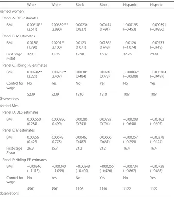
We start by reporting baseline results for married (Table 2) and single (Table 3) men and women. These tables report the coefficients of BMI in hours of work regressions for women (panels A, B, and C) and men (panels D, E, F) using three techniques: OLS, IV (the instru-mental variable being same-sex sibling BMI), and sibling FE (fixed effects). In the case of the IV regressions, the first-stage F test for the instrument range from 16.4 (for married
Table 2BMI coefficients in log hours of work regressions for married respondents: OLS, IV, and FE estimates
White White Black Black Hispanic Hispanic
Married women
Panel A: OLS estimates
BMI 0.00610** (2.511) 0.00659*** (2.890) 0.00236 (0.837) 0.00414 (1.491) − 0.00195
(−0.453) −
0.000391 (−0.0956) Panel B: IV estimates
BMI 0.0180* (1.790) 0.0201** (2.100) 0.0123 (1.071) 0.0186* (1.648) − 0.0126
(−1.074) −
0.00733 (−0.619) First-stage
F-stat
32.13 31.96 17.98 16.87 32.26 29.48
Panel C: sibling FE estimates
BMI 0.00746** (2.221) 0.00767** (2.407) 0.00309 (0.484) 0.00240 (0.373) − 0.000475
(−0.0608) −
0.000384 (−0.0497) Control for
wage
No Yes No Yes No Yes
Observations
5239 5239 1210 1210 1061 1061
Married Men
Panel D: OLS estimates
BMI 0.000550 (0.284) 0.000956 (0.490) 0.00286 (0.743) 0.00292 (0.794) − 0.00208
(−0.640) −
0.00162 (−0.507) Panel E: IV estimates
BMI 0.00356 (0.427) 0.00678 (0.778) 0.00462 (0.487) 0.00606 (0.661) − 0.00257
(−0.299) −
0.00278 (−0.324) First-stage
F-stat
26.8 25.7 21.2 21.2 16.4 16.4
Panel F: sibling FE estimates
BMI −0.00346
(−1.115) −
0.00340
(−1.099) −
0.00248
(−0.402) −
0.00255
(−0.426) −
0.00734
(−0.867) −
0.00728 (−0.865) Control for
wage
No Yes No Yes No Yes
Observations
4561 4561 1196 1196 1122 1122
Hispanic men in Table 3 (E)) to 107.2 (for single White women in Table 4 (A)), suggesting that the instrument is strong by conventional standards.9The first two columns are for Whites, the next two for Blacks, and the last two for Hispanics. Columns 1, 3, and 5 do not include hourly wage rate as a control, while columns 2, 4, and 6 do. Our discussion focuses on the results controlling for own wage, for these results are more likely to indicate causal effects related to marriage markets. To keep the estimates comparable, we use the same samples for regressions using different methods. Hours of work are in logarithmic form.
4.1.1 The married
The OLS results from column 2 in Table 2 (panel A) suggest that among White women, a one-unit increase in BMI is associated with a statistically significant 0.66% increase in
Table 3BMI coefficients in log hours of work for single respondents: OLS, IV, and FE estimates
White White Black Black Hispanic Hispanic
Single women
Panel A: OLS estimates
BMI 0.00451** (2.463) 0.00581*** (3.246) 0.00668*** (4.365) 0.00682*** (4.496) − 0.00120
(−0.359) −
0.000336 (−0.105) Panel B: IV estimates
BMI 0.0104* (1.835) 0.0138** (2.416) 0.00308 (0.458) 0.00452 (0.690) 0.00936 (0.919) 0.0101 (1.050) First-stage F-stat
107.2 101.9 45.8 45.6 32.7 32.6
Panel C: sibling FE estimates
BMI −0.00215
(−0.782)
−0.00172 (−0.628)
0.00504* (1.809) 0.00439 (1.591) 0.00507 (0.913) 0.00523 (0.948) Control for wage
No Yes No Yes No Yes
Observations
6469 6469 4671 4671 2020 2020
Single men
Panel D: OLS estimates
BMI 0.00345* (1.927) 0.00306* (1.777) 0.00603** (2.331) 0.00450* (1.723) 0.00173 (0.746) 0.00201 (0.935)
Panel E: IV estimates
BMI 0.0186** (2.540) 0.0185** (2.558) 0.00225 (0.293) 0.00170 (0.227) 0.00151 (0.164) 0.00283 (0.329) First-stage F-stat
63.8 63.6 85.5 84.9 42.0 41.9
Panel F: sibling FE estimates
BMI 0.000333
(0.118)
−0.000174 (−0.0634)
0.00564 (1.572)
0.00385 (1.095)
−0.00155 (−0.467)
−0.00156 (−0.481) Control for
wage
No Yes No Yes No Yes
Observations
8648 8648 4777 4777 2997 2997
hours worked.10The estimate in column 1, not controlling for wage, is similar, suggesting that if there is an effect of BMI on hours worked, not much of it is channeled via effects of BMI on wage.
When applying the sibling FE method to our sample of married White women, we obtain results similar in size and significance to those obtained with OLS (comparing panels A and C Table 3). Furthermore, when we use the IV method (panel B) and control for wage, we continue to get results significant at the 5% level, but the estimated coeffi-cient is larger than the OLS one: a one-unit increase in BMI leads to an almost 2% increase in White married women’s hours of work (comparing panels A and B, column 2). Therefore, for White married women, the finding of a positive relation between body weight and hours of work is robust to the method of estimation. When own weight is instrumented with sibling’s weight, we get larger effects. One possible explanation for this pattern may be the following: suppose women with higher BMI value leisure more (i.e., work less). Since we do not observe preference for leisure, this is going to create a negative correl-ation between hours worked and BMI, thereby creating a downward bias in the OLS esti-mate. In IV regressions, we are using the sibling’s BMI to predict the BMI of a woman, and therefore, IV estimates do not suffer from this omitted-variable induced endogeneity bias.
Columns 3 to 6 in Table 3 (panel A) report OLS estimates for Black and Hispanic mar-ried women. Samples here are smaller, and the only significant coefficient is that for Black women (when we use IV and control for wage). Panels D–F of Table 3 report results for married men. Here, none of the BMI coefficients are statistically significant, regardless of whether men are White, Black, or Hispanic and regardless of method of estimation.
Table 4BMI and hours work in men and women: does marital status matter?
White White Black Black Hispanic Hispanic
Panel A: OLS estimates for the interaction model, women
BMI 0.00528*** (2.909) 0.00661*** (3.742) 0.00668*** (4.407) 0.00690*** (4.579) − 0.00130
(−0.403) −
0.000624 (−0.202)
Married −0.0895
(−1.312)
−0.0758 (−1.162)
0.155 (1.563) 0.0690 (0.739)
−0.0293 (−0.218)
−0.104 (−0.777) BMI ×
married −
1.44e−05
(−0.00522) −
0.000761
(−0.287) −
0.00502
(−1.452) −
0.00279 (−0.847)
1.63e−05 (0.00342)
0.00309 (0.663)
Control for wage
No Yes No Yes No Yes
Observations
11,708 11,708 5881 5881 3081 3081
Panel B: OLS estimates for the interaction model, Men
BMI 0.00386** (2.136) 0.00361** (2.072) 0.00629** (2.463) 0.00492* (1.911) 0.00167 (0.729) 0.00195 (0.904)
Married 0.223*** (3.320) 0.169** (2.515) 0.375*** (2.943) 0.270** (2.241) 0.218** (2.221) 0.132 (1.362) BMI × married −0.00427* (−1.647)
−0.00320 (−1.247)
−0.00740 (−1.630)
−0.00560 (−1.309)
−0.00253 (−0.754)
−0.00118 (−0.364) Control for
wage
No Yes No Yes No Yes
Observations
13,209 13,209 5973 5973 4119 4119
In sum, we find that White married women with higher BMI work more hours in the labor market using all three methods of estimation. We do not find such effects of BMI for minority married women or for married men. The finding for White married women is consistent with the framework presented in Section 2: thinner women get a higher price in marriage and thus obtain more access to con-sumption or more in-marriage financial transfers. The ethnic differential is consist-ent with the possibility that relative to White women, minority women are less likely to obtain in-marriage financial transfers or access to consumption.11 The gender differential may be a function of the higher involvement of married women in household production and their lower earnings relative to that of married men and to the ensuing higher likelihood that they are on the receiving side of intra-marriage financial transfers.
4.1.2 The singles
Table 3 reports results for single women (panels A–C) and for single men (panels D–F). The OLS results from column 2 (panel A) suggest that among White single women, a one-unit increase in BMI is associated with a statistically significant 0.58% increase in hours worked (0.45% if hourly wage is not added as a control variable; column 1, Table 3, panel A). Comparing panel A with panel B indicates that a one-unit increase in BMI has a larger effect when the IV method is used: a one-unit increase in BMI leads to a 1.38% (column 2, panel B) increase in hours worked. The estimate is significant at a 5% level of significance. Thus, as in the case of White married women, both OLS and IV estimates suggest that heavier White single women work more hours. However, we do not find any significant results when the sibling FE method is used. One potential reason may be that the correlation between own BMI and sib-ling BMI is stronger (as suggested by larger first-stage F-stats for single women), and therefore, differencing may magnify the measurement error (Deaton 1995), rendering the estimates insignificant. OLS results also suggest that Black single women with higher BMI work more hours. This result is also robust to inclusion of wage.
OLS results in Table 3 (panels D and E) suggest that BMI is also positively asso-ciated with hours of work of White and Black single men. The result for White single men carries over when the IV method is applied (columns 1 and 2), but that is not the case for Black single men (columns 3 and 4). As for Hispanics, we find no association between body weight and hours of work for either single men or single women.
4.1.2.1 Comparing results with and without control for wage Our results suggest
4.1.3 Comparing results for married and single respondents
In the case of White women, the coefficients of BMI are similar for single women and married women. This holds using both the OLS and IV methods. For instance, using the IV method and controlling for wage, a one-unit increase in BMI leads to a 1.38% increase in hours worked by single women and a 2% increase in hours worked by mar-ried women. Both findings are significant at the 5% level of significance. This suggests that single women anticipate possible future benefits from being married, with heavier single women anticipating lower financial in-marriage transfers. To test whether the effect of BMI on hours of work is different in single and married respondents, we pooled the single and married samples, separately for each ethnic group, and included married status and an interaction between marital status and BMI in OLS regressions. We use OLS (and therefore ignore the endogeneity of BMI as well as marriage) as the purpose of these exer-cises is to check whether the level of association between BMI and hours of work varies by marital status. Table 4 reports the results for women (panel A) and men (panel B). We only report the coefficients of BMI, marital status, and the interaction between BMI and marital status. We list all other control variables below the table. Table 4 (panel A) shows that high-BMI women (White or Black) work more in the combined sample. Being mar-ried does not make a significant difference in women’s hours worked, suggesting that marital status itself does not change hours of work. Most importantly, the coefficient of the interaction term is never significant, suggesting that the level of association between BMI and hours of work does not vary with marital status.
Results for men (panel B) are somewhat different from the results for women. Tables 2 and 3 suggest this as well. Married men work more, and the coefficient of the interaction between BMI and marital status is significant for White men when we do not control for wage (column 1). However, once we control for wage (column 2), it is not significant anymore. One possible explanation is that high-BMI single men need more resources to attract potential mates, but once they are married, they do not face the need for the extra resources. This is consistent with the findings in Mukhopadhyay (2008).
It thus appears that in the case of Black and White men, as well as in the case of Black women, there is positive association between BMI and hours of work at the single stage, but not at the married stage. The only case where a positive association between BMI and hours of work is also observed at the married stage (and possibly larger for the marrieds than for the singles) is the case of White women. White women may be the exception for they may be more likely to receive in-marriage transfers from husbands compared to their Black or Hispanic counterparts. Therefore, there may be more of an in-marriage financial reward (or a reward in the form of extra access to consumption) for being thin in the case of married White women than in the case of married minority women. The result that the association between BMI and hours of work disappears for Black married women at the married state is consistent with Black women often being the principal earner in their couple (see Mincy et al. 2005). This may also reflect that married women’s access to their husband’s financial resources may vary across races (see Grossbard 2005).
4.2 Are marriage markets driving the relation between BMI and hours of work in women?
4.2.1 Married women
In the conceptual framework section (Section 2), we discussed that marriage markets can affect the relationship between BMI and hours of work through two potential chan-nels. First, high BMI may mean lower spousal income. Second, conditional on spousal income, high BMI may mean lower bargaining power within marriage, i.e., less access to spousal income.12Therefore, our next step is to use data on married women and to estimate the association between women’s BMI and their spouse’s annual income (in $10,000). We also estimate whether the association between BMI and hours of work in married women is sensitive to inclusion (or lack thereof ) of spousal characteristics (age, education, and annual income) in OLS regressions of hours of work.
Table 5 shows the results. Panel A presents the association between BMI and spouse’s annual income, and panel B presents the association between BMI and hours of work, with and without spousal characteristics. All regressions include all women’s characteris-tics including her wage. Columns 1, 3, and 5 (of panel A) only include women’s character-istics, whereas columns 2, 4, and 6 (of panel A) include the husband’s age and education as additional controls. Results in panel A show that for married White women, the coeffi-cient of BMI is−0.112 (column 1), or in other words, a one-unit increase in BMI is associ-ated with $1120 reduction in annual spousal income. Controlling for spouse’s age and education has little effect on the estimate. The coefficient of BMI is not significant for married Black women regardless of inclusion of age and education, and it is not significant in married Hispanic women when we include the husband’s age and education. This sug-gests that there is more of a material payoff for being thin in the case of White married women than in the case of Black or Hispanic married women.
Columns 2, 4, and 6 (of panel B) reproduce the OLS results reported in the correspond-ing columns of Table 2 (panel A). The followcorrespond-ing characteristics of the husband had been
Table 5BMI, spousal annual income, and log hours of work for married women
White White Black Black Hispanic Hispanic
Panel A: BMI and spousal annual income
BMI −0.112***
(−3.885)
−0.108*** (−3.772)
−0.0396 (−0.947)
−0.0177 (−0.405)
−0.118** (−2.192)
−0.0459 (−0.993) Control for wife’s
characteristics
Yes Yes Yes Yes Yes Yes
Control for husband’s characteristics
No Yes No Yes No Yes
Observations 5239 5239 1210 1210 1061 1061
Panel B: BMI and hours of work with and without spousal characteristics
BMI 0.00702***
(3.112)
0.00659*** (2.890)
0.00403 (1.410)
0.00414 (1.491)
0.000248
(0.0641) −
0.000391 (−0.0956) Control for own
wage
Yes Yes Yes Yes Yes Yes
Control for spousal characteristics
No Yes No Yes No Yes
Observations 5239 5239 1210 1210 1061 1061
included: age, education, and annual income. Columns 1, 3, and 5 present results for the same regressions excluding the characteristics of the husband. Results show that the coef-ficients of BMI are unaffected by the addition of spousal characteristics. This suggests that high-BMI White women work more hours not because they are married to men earning less, but that they have less bargaining power in marriage and can access less of their spouse’s income. This is consistent with results reported by OQD.
4.2.2 Single women
Our results so far suggest that the association between BMI and hours of work in single women stems from how BMI affects expectations about marriage. For single women, we cannot pursue the direct strategy employed in Table 5 above. Instead, we investigate the rational expectations argument presented above by performing two more tests: (1) we use a unique question about marriage expectations and (2) we investigate how the association between BMI and single women’s hours of work changes when we control for predicted cumulative spousal income.
First, we use a question that was asked to the single NLSY97 respondents in some of the waves (2000, 2001, 2009, 2010, and 2011). The respondents were asked “Now think about five years from now, you will be [{AGE IN 5YRS}]. What is the percent chance that you will be married?”This question was not asked in the NLSY79, and therefore, this analysis can only be performed on NLSY97 women. As we discussed earlier, our hypothesis is that single women with high BMI expect smaller future income transfer from husbands, and therefore, they work more in the labor market even when they are single. It follows that the effect of BMI will be stronger in single women with higher self-assessed probability of getting mar-ried in the next 5 years, compared to their counterparts who have a lower self-assessed probability of getting married in the next 5 years. In a different but relevant context, Kur-eishi and Wakabayashi (2013) showed that marriage expectations could affect single women’s savings decisions: they found that single women who expect to get married save significantly less than single women who do not expect to get married in the next 3 years.
Accordingly, we re-estimate the OLS regressions for single women, controlling for prob-ability of marriage. We add an interaction term between the self-assessed probprob-ability of mar-riage and BMI. This regression has the same set of control variables (including log wage) as in Table 3. However, sample sizes are smaller given that we only used the NLSY97 and that only selected waves of NLSY97 included the question about marriage expectations.
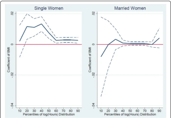
Figure 1 shows the marginal effect of BMI for single women and how it varies with the self-assessed probability of marriage, along with the 95% confidence interval. Panel A suggests that for single White women, the marginal effect of BMI on hours of work is insignificant when the expected probability of marriage is zero. The association between BMI and hours of work remains statistically insignificant as long the chance of getting married remains below 40%. However, the marginal effect is positive and signifi-cant for single White women when the chance of getting married in the next 5 years is at 50% or above. Panel B (panel C) shows the marginal effect of BMI for Black (Hispanic) single women. Results here are never statistically significant.
annual income of the spouse and number of years the woman was married. If a woman was never married by the time of the last interview, then her cumulative spousal in-come is zero. We regress cumulative spousal inin-come on the characteristics of women including their BMIs. Results (not shown) suggest that for White women, a one-unit increase in BMI is associated with $11,610 less in cumulative spousal income,13but we do not find any association for Black women. We then use the estimated coefficients to obtain the predicted cumulative spousal income of single women. Then we run regres-sions for single women in the entire NLSY data sets, with and without including this predicted cumulative spousal income.
Table 6 presents OLS regressions for single women. All regressions include all the controls used in Table 3, including their own wage. Thus, columns 1, 3, and 5 in this table reproduce the results presented in columns 2, 4, and 6 of Table 3 (panel A). In the regression results re-ported in columns 2, 4, and 6 of Table 6, we have added predicted cumulative spousal income as an additional control. Results show that for White single women, the coefficient of BMI goes down from 0.00581 to 0.00373 when we add predicted cumulative spousal income as an additional control. This suggests that one of the mechanisms by which BMI influences single White women’s hours of work is via BMI’s effect on predicted spousal income. However, this is not the case for Black single women: here, the effect of BMI does not seem to act via its ef-fect on predicted spousal income: the coefficients of BMI in columns 3 and 4 of Table 6 are very similar. In the case of Hispanic women, we find no association in both columns 5 and 6.
Adding up the results reported in Fig. 1 and Table 6, it appears that one reason why higher-BMI White single women work more in the labor market relative to their lower-BMI counterparts is that they expect lower future in-marriage income transfers. In turn,
these expected future in-marriage transfers are lower because either heavier women are likely to get married to men with fewer resources or heavier women have less access to spousal resources14 (i.e., a lower bargaining power). It seems that in the case of White women, both of these channels operate.
4.3 Can labor market mechanisms explain the relation between BMI and hours of work in single women?
In our Section 2, we discussed two additional labor market-based mechanisms that can explain the positive association between BMI and hours of work in single women. First, is it possible that high-BMI women are less healthy, and unhealthy women expect to spend fewer years in the labor force at older ages and therefore they work more hours at an early age to compen-sate for a shorter expected working span. Since the single sample is substantially younger than the married sample, we are most likely to observe this in the single sample. A second possibil-ity is that high-BMI singles are more likely to work full time in order to qualify for health in-surance benefits.15
Next, we check whether these mechanisms can explain the relation between BMI and hours of work in women. First, we exclude individuals who report fair or poor health or have any kind of work limitations from our samples of single women (about 4% of the sample). Then we estimate the same OLS regressions to check whether the association between BMI and hours of work differs from the results we reported in Table 3. Results presented in Table 7 suggest that when we exclude women with health problems, our results still hold. Thus, it is unlikely that poor health explains the association between hours of work and BMI.
Next, we test whether our results for single women are driven by considerations related to access to health insurance. We estimate the association between BMI and hours of work separately for two groups: those with employers who offer health insurance as a benefit and
Table 6BMI and log hours of work for single women: with and without predicted cumulative spousal income
White White Black Black Hispanic Hispanic
BMI 0.00581***
(3.246)
0.00373* (1.825)
0.00682*** (4.496)
0.00634*** (4.086)
−0.00033
(−0.105)
−0.00059
(−0.182)
Control for own wage Yes Yes Yes Yes Yes Yes
Control for predicted cumulative spousal income
No Yes No Yes No Yes
Observations 6469 6469 4671 4671 2020 2020
Note 1: Control variables include work experience (quadratic), educational categories, dummies for whether the woman believes in traditional gender roles, whether the woman has any children, if the youngest child is below six, yearly age dummies, region of residence dummies, and year dummies. Note 2: Allt-stats reported are based on standard errors clustered at the individual level. ***p< 0.01, **p< 0.05, and *p< 0.10
Table 7BMI and log hours of work for single women: excluding women with health limitations
White White Black Black Hispanic Hispanic
BMI 0.00588***
(3.469)
0.00702*** (4.189)
0.00680*** (4.341)
0.00701*** (4.490)
−0.00128
(−0.379)
−0.000474
(−0.147)
Control for wage
No Yes No Yes No Yes
Observations 6296 6296 4486 4486 1983 1983
those with employers who do not offer health insurance.16Table 8 reports coefficients of BMI in OLS regressions of hours of work for single women. All regressions include the standard set of controls including wage. Table 8 shows that the positive association of BMI and hours of work holds in both groups of single White women and single Black women. The smaller coefficient of BMI for White women with employer-provided insurance can be explained by the fact that most of these women already work full time (on an average 2008 vs. 1235 h/year for women do work for employers that do not offer health insurance), often a requirement to eligibility for such insurance. Therefore, there is not much room for additional hours of work. The group of women who do not have employer-provided health insurance is illuminating. These women’s hours of work are unlikely to be motivated by in-surance (since the employer do not offer health inin-surance in the first place), but the positive BMI per hours of work coefficient is nevertheless found for them too.
4.4 Robustness checks
We perform a number of robustness checks. First, all results reported so far were esti-mated for samples excluding respondents without siblings. Therefore, we re-estimate OLS regressions in Tables 2 and 3 for full samples, including those without any siblings. The results (presented in Table 10 in the Appendix) are qualitatively similar to those reported in panel A of Tables 2 and 3.
Second, we experiment with alternative assumptions about extreme values of BMI. As we discussed in Section 3, Winsorizing BMI (at 1%) involves replacing all BMI below 17.2 by 17.2 and replacing all BMI above 45.5 by 45.5. Here, we follow two alternative strategies: first, we ignore all BMIs that are below 17.2 or above 45.5, and second, we ignore all BMIs that are below 18.5 or above 40.0 (a strategy followed by OQD). Table 11 in the Appendix shows results using our three methods of estimation (OLS, IV, and sibling FE) when using these two alternative strategies, along with our baseline results. The results show that our results are robust to these alternative approaches.
Third, we check whether the association between BMI and hours of work varies across the hours of work distribution by using the UQR method described in Section 3. To the extent unobserved characteristics are responsible for different women choosing different hours of work, UQR can be a check on whether the OLS results are driven by this type of unobserv-able factors. An added benefit of using UQR is that it can help us infer whether health insur-ance motive is driving the association between BMI and hours of work. If the health insurance motive is the driving factor behind this association, then we are likely to see the ef-fect in people who are right below the cutoff of health insurance eligibility (which is about 30 h/week or about 1500 h/year). The 1500 h/year is between the 40th and 50th percentile,
Table 8BMI and log hours of work for single women:by availability of employer-provided insurance
White women Black women Hispanic women
Employer offers ins.
Employer does not offer ins.
Employer offers ins.
Employer does not offer ins.
Employer offers ins.
Employer does not offer ins.
BMI 0.00263* (1.960) 0.00975*** (3.174) 0.00513*** (3.684) 0.00506* (1.921) −0.000602 (−0.248) 0.00301 (0.419)
Observations 3232 2221 2759 1451 1044 749
depending on the race/marital status group. In contrast, if the marriage market is the driving force behind the association between BMI and hours of work, then we are likely to see an ef-fect at all levels of hours of work. Figure 2 shows the coefficient of BMI and how it varies across the unconditional log (BMI) distribution for White women. The left panel is for single women, and the right panel is for married women. Figure 2 shows that the effect of BMI is positive and significant over most of the distribution for both single and married White women. The coefficient of BMI seems to be highest well before the 40th percentile for both single and married White women. This suggests that the health insurance motive is unlikely to explain the pattern represented in Fig. 2. Figures 3 and 4 present the corresponding re-sults for Black and Hispanic women. Consistent with our OLS rere-sults, we find that the coef-ficient of BMI is positive and significant for single Black women over most of the distribution, while it is never significant for married Black women or for Hispanic women.
Fourth, in our analyses so far, we assumed that the relation between BMI and hours worked is linear. This assumption may not be accurate, and if the true relationship is non-linear, this may introduce bias in our estimates. To address this issue, we estimate a partially linear model where BMI enters the“hours worked”equation non-parametrically. We use Robinson’s (1988) double residual estimator.17Figure 5 presents the results from semiparametric regressions in which we treat BMI as an exogenous variable. The left panel shows the results for single women and the right panel for married women. To show the difference in the semiparametric fit across races, we do not include the 95% confidence interval in this figure. The left panel in Fig. 5 indicates that the relationship is broadly linear (and monotonic) until a BMI of 40 in the case of both White and Black single women. Beyond that, an increase in BMI is associated with a decline in hours worked, most likely because the health effects dominate other
Fig. 3BMI and log hours of work for Black women:Unconditional Quantile regression estimates (with 95% confidence interval). Note: Control variables include work experience (quadratic), educational categories, dummies for whether the woman believes in traditional gender roles, whether the respondent has any children, if the youngest child is below six, yearly age dummies, region of residence dummies, and year dummies. For the married sample, additional controls include spouse’s age, educational categories, and annual income
considerations. The semiparametric estimates for married White women (right panel of Fig. 5) suggest more evidence of non-linearity. Even in this case, the estimated increase in hours of work when BMI doubles from 20 to 40 is not statistically different from the OLS estimate.
Fifth, following a common practice in this literature, we created dummies for weight cat-egories, to replace the linear BMI variable. We followed the literature and created four weight categories: underweight (BMI < 18.5), healthy weight (18.5 ≤ BMI < 25), overweight (25≤BMI < 30), and obese (BMI≥30). Then we estimated OLS regressions with weight cat-egories as our independent variables of interest, with healthy weight as the omitted category and controlling for wage. The results from these regressions are presented in Table 12 in the Appendix. Results suggest White and Black women who are either overweight or obese work more hours than their healthy weight counterparts. This holds for single and married women. As for men, the overweight single men work more hours, but the obese do not.18
Finally, so far we have focused on hours of work as our outcome variable and ignored the extensive margin or labor supply. It is also conceivable that BMI affects the labor-force partici-pation decision. The estimates reported in Table 13 in the Appendix are from OLS and IV re-gressions. We tried to estimate the corresponding probit and probit models, but the IV-probit likelihood does not converge in two out of six cases (single Black women and married Hispanic women). Since Angrist and Pischke (2009) argue that “IV methods capture local average treatment effects regardless of whether the dependent variable is binary, non-negative, or continuously distributed on the real line,”we report the estimates from linear IV models. Results shown in Table 13 in the Appendix suggest that BMI increases probability of employ-ment in single White women (using OLS) and in married White women (using IV). We do not find any consistent pattern of relationship between BMI and employment probability.
5 Conclusions
To examine whether body weight is associated with hours of work in the labor market and possible causal links behind this association, we analyze US data from the NLSY79 and NLSY97. We use OLS, IV (with sibling BMI serving as an instrument for own BMI), and sibling FE regressions. Higher body weight (BMI) could affect hours of work via mechanisms related to labor markets or marriage markets. Our conceptual framework leads us to expect that hours of work will be associated positively with body weight as part of marriage market processes rewarding thinness, including in-marriage transfers. Given traditional gender roles, married women would be more likely to receive intra-marriage income transfers than married men, and thus, the hours of work of married women would be associated more positively with high BMI than the hours of work of married men. We find that using the IV method and controlling for wage, a one-unit increase in BMI leads to an almost 2% increase in White married women’s hours of work, but BMI is not associ-ated with hours of work of married men. This is consistent with our marriage market in-terpretations and dominance of traditional gender roles over egalitarian roles. We also raise the possibility that White married women benefit more from intra-marriage trans-fers than minority married women, possibly as a function of racial discrimination in mar-riage markets. Our findings of a strong association between BMI and hours of work for White married women, but no such association for Black or Hispanic married women, are consistent with the existence of ethnic discrimination in marriage markets.
Our conceptual framework also leads us to expect that the hours of work of singles will vary with BMI. To the extent that higher BMI is associated with lower prospects of being in couple and obtaining intra-couple transfers, body weight would increase singles’willingness to work in labor markets. We find that using the IV method and controlling for wage, a one-unit increase in BMI leads to a 1.4% increase in White single women’s hours of work. This finding is consistent with single White women expecting marriage to bring them a flow of future in-marriage transfers and with these transfers being related to thinness.
We examine whether a negative association between BMI and spousal income can ex-plain the positive link between BMI and women’s hours of work. We find that for White married women, the association between BMI and hours of work remains significant even after controlling for spousal characteristics, including income. This suggests that high-BMI married women have less access to spousal income, conditional on that spousal income. This suggests a negative association between body weight and in-marriage bargaining power, price in marriage, or in-marriage financial transfers. We also show that the positive associ-ation between BMI and hours of work of White single women increases with self-assessed probability of future marriage and varies with expected cumulative spousal income. These findings reinforce the rational expectation interpretation according to which singles take future prospects of in-marriage transfers into account when determining their hours of work. Our finding of a positive association between hours of work and BMI of White single men could indicate that some men also receive transfers in marriage, implying that women pay the price of marriage. For instance, overweight single men may work more hours in the labor force than men of normal weight because they are less likely to marry a woman who transfers some of her income to them. It may also indicate that high-BMI men may need more income to attract potential spouses.
We also test several alternative (non-marriage market) mechanisms that could result into a positive relationship between BMI and hours of work: a connection between BMI and health limitations and an association between BMI and health insurance. Neither of these mechanisms seems to explain the observed relationship between BMI and hours of work.
The positive association that we find between hours of work and body weight carries implications for policy. Exercising and good nutrition may not only be beneficial in view of their well-known effects on health outcomes but also due to their contribution to the personal disposable income of individuals who are either married or planning to marry.
We hope that future research will investigate this topic using other data sets, includ-ing data on the weight of both spouses and siblinclud-ings. It would also be interestinclud-ing to see if similar results are obtained for other countries. To the extent that it uncovers a premium for thinness in marriage markets, future research could establish whether it varies cross-culturally.
Endnotes
1
See Grossbard (2015, Chap. 4) for a review of more recent research on this theme.
2
See Grossbard (2015, Chap. 5) for a review of more recent research on this theme.
3
More on this distinction between the models in Grossbard (2011, 2015)
4
Winsorizing replaces all the values of a particular variable at both tails of the distribution by a specified value. In our case, we replace all BMI values below the 1st percentile of BMI distribution (17.2) with a BMI value of 17.2. We also replace all BMI values above the 99th percentile (45.5) with a BMI value of 45.5. This allows us to use the extreme observations without outliers having a big impact on the estimates. For a more detailed discussion, see Barnett and Lewis (1994).
5
We show robustness of our results to other reasonable approaches to extreme BMI values in Table 11 in the Appendix.
6
Table 9 in the Appendix presents the summary statistics for men.
7
We thank an anonymous referee for suggesting we also use this strategy.
8
Note that this is different from traditional quantile regression, which shows how parameter estimates vary across the conditional distribution of the dependent variable.
9
In Section 3.2, we have discussed the threats to exclusion restriction. We also discussed why we believe the exclusion restriction is valid here. Since we have only one instrument, we cannot do an over-identification test. Instead, as an ad hoc test, we include sibling BMI (along with own BMI) in the outcome equation. In these regressions, sibling BMI is never statistically significant.
10
Full results of all regressions are available upon request.
11
This finding could also be interpreted in terms of the Black-White cultural differ-ence theory (Averett and Korenman 1999).
12
We thank an anonymous reviewer for pointing this out to us.
13
This estimate is about 10 times as large as the estimate reported in Table 5. This is expected as the estimate in Table 5 is for annual income of a spouse, whereas this esti-mate is for expected cumulative spousal income.
14
We thank an anonymous reviewer for pointing this to us.
15