Service workload patterns for Qos-driven cloud resource management

R E S E A R C H

Open Access

Service workload patterns for Qos-driven

cloud resource management

Li Zhang

, Yichuan Zhang

, Pooyan Jamshidi

, Lei Xu

and Claus Pahl

Abstract

Cloud service providers negotiate SLAs for customer services they offer based on the reliability of performance and availability of their lower-level platform infrastructure. While availability management is more mature, performance management is less reliable. In order to support a continuous approach that supports the initial static infrastructure configuration as well as dynamic reconfiguration and auto-scaling, an accurate and efficient solution is required. We propose a prediction technique that combines a workload pattern mining approach with a traditional collaborative filtering solution to meet the accuracy and efficiency requirements. Service workload patterns abstract common infrastructure workloads from monitoring logs and act as a part of a first-stage high-performant configuration mechanism before more complex traditional methods are considered. This enhances current reactive rule-based scalability approaches and basic prediction techniques by a hybrid prediction solution. Uncertainty and noise are additional challenges that emerge in multi-layered, often federated cloud architectures. We specifically add log smoothing combined with a fuzzy logic approach to make the prediction solution more robust in the context of these challenges.

Keywords: Quality of service, Resource management, Cloud scalability, Web and cloud services, QoS prediction, Workload pattern mining, Uncertainty

Introduction

Quality of Service (QoS) is the basis of cloud service and resource configuration management [1, 2]. Cloud service providers – whether at infrastructure, platform or soft-ware level – provide quality guarantees usually in terms of availability and performance to their customers in the form of service-level agreements (SLAs) [3]. Internally, the respective service configuration in terms of avail-able resources then needs to make sure that the SLA obligations are met [4]. To facilitate SLA conformance, virtual machines (VMs) can be configured and scaled up/down in terms of CPU cores and memory, deployed with storage and network capabilities. Some current cloud infrastructure solutions allow users to define rules man-ually to scale up or down to maintain performance levels.

*Correspondence: [email protected]

2IC4/School of Computing, Dublin City University, Dublin, Ireland Full list of author information is available at the end of the article

QoS factors like service performance in terms of response time or availability may vary depending on net-work, service execution environment and user require-ments, making it hard for providers to choose an initial configuration and scale this up/down to maintain the SLA guarantees, but also optimising resource utilisation at the same time. We utilise QoS prediction techniques here, but rather than bottom-up predicting QoS from moni-tored infrastructure metrics [5–7], we reverse the idea, resulting in a novel technique for pattern-based resource configuration.

A pattern technique is at the core of the solu-tion. Various types of cloud computing patterns exist [8], covering workload, but also offer types and appli-cation and management architectures. These patterns link infrastructure workloads such as CPU utilisation with service-level performance. Recurring workloads have already been captured as patterns in the liter-ature [8], but we additionally link these to service quality.

We determine service workload patterns through pattern mining from resource utilisation logs. These service workload patterns (SWPs) correspond to typi-cal workloads of the infrastructure and map these to QoS values at the service level. A pattern consists of a relatively narrow range of metrics measured for each infrastructure concern such as compute, mem-ory/storage and network under which the QoS con-cern is stable. This can be best illustrated through utilisation rates. Should resources be utilised in a certain range, e.g., low utilisation of a CPU around 20 %, then the response-time performance can be expected to be high and not impacted negatively by the infrastructure.

These patterns can then be used in the follow-ing way. In a top-down approach, we take a QoS requirement and determine suitable workload-oriented configurations that maintain required values. Further-more, we enhance this with a cost-based selection function, applicable if many candidate configurations emerge.

We specifically look at performance as the QoS concern here since dealing with availability in cloud environments is considered as easier to achieve, but performance is cur-rently neglected in practice due to less mature resource management techniques [4]. We introduce pattern min-ing mechanisms and, based on a QoS-SWP matrix, we define SWP workload configurations for required QoS. The accuracy of the solution to guarantee that the chosen (initially predicted) resource configurations meet the QoS requirements is of utmost importance. An appropriate scaling approach is required in order to allow this to be utilised in dynamic environments. In this paper, we show that the pattern-based approach improves the efficiency of the solution in comparison with traditional predic-tion approaches, e.g., based on collaborative filtering. This enhances existing solutions by automating current manual rule-based reactive scalability mechanisms and also advances prediction approaches for QoS, making them applicable in the cloud with its accuracy and performance requirements.

Cloud systems are typically multi-layer architectures with services being provided at infrastructure, platform or software application level. Uncertainty and noise are additional challenges that emerge in these multi-layered, often federated clouds architectures. We extend earlier work [9] to address these challenges. We pro-pose to use log smoothing and a fuzzy logic-based approach to make the prediction solution more robust in the context of these challenges. Smoothing will deal with log data variability and will allow detect-ing trends (but adds more noise). Uncertainty often occurs as to the completeness and reliability of mon-itored data, which will here be addressed through

a fuzzy logic enhanced prediction. We will demon-strate the robustness of the solution against noise and uncertainty.

Section ‘Quality-driven configuration and scaling’ outlines the solution and justifies its practical

rel-evance. Section ‘Workload patterns’ introduces

SWPs and how they can be derived. Section ‘Quality pattern-driven configuration determination’ discusses the selection of patterns as workload specifications for resource configuration. The application of the solution for SLA-compliant cloud resource configura-tion is described in Secconfigura-tion ‘Pattern-driven resource configuration’. Section ‘Managing uncertainty’ deals with uncertainty through a fuzzification of the pat-terns. Section ‘Evaluation’ contains an evaluation in terms of accuracy, performance and robustness of the solution and Section ‘Related work’ discusses related work.

Quality-driven configuration and scaling

Cloud resource configuration is the key problem we address. We start with a brief discussion of the state-of-the-art and relevant background.

Fig. 1Measured QoS mappings: Infrastructure to Servic ([CPU, network, storage]→Performance)

depending on the infrastructure parameters, but not nec-essarily in a way that would be easy to determine and predict.

The first step is to monitor and record these input met-rics in system-level resource utilisation logs. The second step is pattern extraction. From repeated service invo-cations records (the logs), an association to service QoS values based on prediction techniques can be made. An observation based on experiments that we made is that most services have relatively fixed service workload pat-terns (SWP):

• The patterns are defined here as ranges of storage, network and CPU processing characteristics that reflect stable, small acceptable variations of a QoS value.

• Generally, service QoS keeps steady under a SWP, allowing this stable mapping between infrastructure input and QoS to be used further.

If we can extract SWPs from service logs or the respective resource usage logs (based on pattern min-ing), the associated service quality can be based on usage information using pattern matching and predic-tion techniques. Even if there is no or insufficient usage information for a given service, quality values can be calculated using log information of other sim-ilar services, e.g., through collaborative filtering. These two steps can be carried out offline. The next, first online step is pattern matching, where dynamically a pattern is matched in the matrix against perfor-mance requirements. The final step is the (if neces-sary dynamic) configuration of the infrastructure in the cloud.

The hypothesis behind our workload pattern-driven resource configuration based on required service-level quality is the stability of variations of quality under SWPs. We assume SLA definitions to establish QoS requirements and the charged costs for a service to be decided between provider and consumer. Service-specific workload pattern are mined and constructed which considers environmental characteristics of a service (in a VM) deployment. We experimentally demonstrate

that the hybrid technique for QoS-to-SWP mappings (based on pattern matching and collaborative filtering for missing information) enhances accuracy and com-putational performance and makes it applicable in the cloud. In contrast, traditional prediction techniques can be computationally expensive and unsuitable for the cloud.

We limit this investigation to services and infras-tructure with some reasonably deterministic behaviour, e.g., classical business or technology management applications. However, we deal with larger substantial uncertainties arising from the infrastructure and plat-form environment in which the services are executed. We also focus on the variability of log data, noise that occurs and uncertainties arising from multi-cloud environments.

Workload patterns

The core concept of our solution is a Service Workload Pattern (SWP). A SWP is a group of service invocation characteristics reflected by the utilised resources. In a SWP, the value of workload characteristics is a range. The QoS is meant to be steady under a SWP. We describe a SWPMas a triple of ranges low to high (aslow ∼ high ranges):

M= CPUlow∼CPUhigh, Storagelow∼Storagehigh, Networklow∼Networkhigh

(1)

CPU, Storage and Network are common server

We initially work with monitored absolute figures for CPU time used, stored data size and network throughput. Later on, we also convert this into normalised utilisation rates with respect to the allocated resources.

SWP pattern mining and construction

We assume service-level execution quality logs in the format < q1,. . .,qn > and infrastructure-level resource monitoring logs < r₁i,. . .,r_mi > with i = 1,. . .,j for j different quality aspects (e.g., storage, network, server CPU utilisation) of the past invocations of the services under consideration, as illustrated in Fig. 1. For each service, the resource metrics and the associ-ated measured performance are recorded. The challenge is now to determine or mine combinations of value ranges for input parameters r that result in stable, i.e., only slightly varying performances. The solution is a SWP extraction process that constructs the workload patterns.

• A SWP is composed of storage, network and computation characteristics. For these, we take throughput, data size and CPU utilization as representatives, respectively.

• We consider the execution (response) time as the representative of QoS here.

An execution log records the input data size and exe-cution QoS; a monitoring log records the network status and Web server status. We reorganize these two logs to find the SWP under which QoS keeps steady. Our SWP mining algorithm is based on a generic algorithm type, DBSCAN (density-based spatial clustering of applications with noise). DBSCAN [10] analyses the density of data and allocates the data into a cluster if the spatial density is greater than a threshold. The DBSCAN algorithm has two parameters: the threshold ε and the minimum number of points MinPts. Two points can be in the same clus-ter if their distance is less thanε. The minimum number of points is also given. We also need a parameter Max-TimeRange, the max time range of a cluster. We expect the range of time is a cluster that can be steady and that has a size limit. When the cluster is too large, e.g., if the range exceeds a threshold, the cluster construction should be stopped. The main steps are given in the following Algorithm 1:

• Select any objectp from the object set S and find the objects setD in which the object is density-reachable from objectp with respect toεandMinPts.

• Choose another object without cluster and repeat the first step

The pattern extraction algorithm is presented in Algorithm 1.

Algorithm 1SWP Extraction Algorithm based on DBSCAN.

Input: Service UsageInforSet(execution+monitoring log),ε,MinPts,MaxTimeRange.

Output: SWPPatternBase, Pattern-QoS information, PatternQoS.

1: for(Infori<CPU,DataSize,ThroughPut,Performance>

∈InforSetdo

2: ifInforidoes not belong to any exist clusterthen

3: Pj=newPattern(Infori) {create a new pattern with Inforias seed}

4:

5: Add(Pj,PatternBase)

6: InforSet=InforSet−Infori

7: SimInfor=SimilarInfor(InforSet,Infori,ε) {SimInfor

is the information set which includes all the similar usage information ofInfori. Differences between the information inSimInforandInforion the character-istics value except execution time are less thanε.nis the number of information items inSimInfor.}

8: InforSet=InforSet−SimInfor

9:

10: ifn>MinPts then

11: {MinPtsis min number of exec info in cluster}

12: (S1,S2. . .,Sm)=Divide(SimInfor) {Divide

SimInforinto different groups.}

13:

14: GroupS1includes all information of services1 15: for(k=1;K≤m;k+ +)do

16: fornj∈Skdo

17: ifMaxTime−MinTime < MaxTimeRange

then

18:

19: SimInfor = SimilarInfor(InforSet, Inforj, time,MinPts,ε){Search similar info ofSk

in execution information set. If the num-ber of similar information item is less than

MinPts, then the density will turn low and top the loop.}

20: Sk=Sk+SimInfor

21: InforSet=InforSet−SimInfor

22: end if

23: end for

24: PatternCharacteristics(Sk) {Organizes the

information in the cluster and statistics for the ranges of characteristics completes matrix}

25: end for

26: end if

27: end if

We give higher precedence to more recent log entries. Exponential smoothing can be applied to any discrete set of sequential observationsxi. Let the sequence of obser-vations begin at time t = 0, then simple exponential smoothing is defined as follows:

y0=x0

yt=αxt+(1−α)yt−1,t>0, 0< α <1 (2)

The choice ofαis important. Close to 1 has no smooth-ing effect and gives higher weight to recent changes and as a result the estimate may fluctuate dramatically. Val-ues ofα closer to 0 have a better smoothing effect and the estimate is less responsive to recent changes. We can choose a value like 0.8 as the default, which is relatively high, but reflects the most recent multi-tenancy situation (which can undergo short-term changes). We will discuss this separately later in more detail in Section ‘Variability and smoothing’.

Pattern-quality matrix

The input value ranges form a pattern that is linked to the stable performance ranges in aQuality Matrix MS(M,S) based on patterns M and services S. MS associates a service quality QoSP(Si,Mi) (with P standing for per-formance) of service Si in S under a pattern Mj in M.

MS=

⎛ ⎜ ⎜ ⎝

S1 S2 . . . Sm M1 q1,1 q1,2 . . . q1,m M2 q2,1 q2,2 . . . q2,m . . . . . . . . . . . . . Ml ql,1 ql,2 . . . ql,m

⎞ ⎟ ⎟

⎠ (3)

Figure 1 at the beginning illustrated monitoring and exe-cution logs that capture low-level metrics (CPU, storage, network) and the related service response time perfor-mance. SWPsMithen result from the log mining process using clustering.

The following is a set of patternsM1toM3for the given example in Fig. 1:

CPU Strg Netw

M1= [2.1∼2.5 , 10∼11 , 0.1∼0.2] M2= [2.0∼2.2 , 8∼30 , 0.2∼0.4] M3= [1.2∼2.0 , 10∼20 , 0.1∼0.5]

(4)

For those patterns, we can construct the following qual-ity matrixMS:

⎛ ⎝

S1 S2 S3

M1 0.2∼0.5s 1.5∼1.8s

M2 1.4∼1.8s 1.1∼1.5s

M3 1.5∼2.1s

⎞

⎠ (5)

The matrixMSabove shows the QoS in this example for performance information of all servicessjfor all patterns Mi. The qualityqij(1 ≤ j ≤ l, 1 ≤ i ≤ m) is the quality

of servicesj under patternMi with the quality valueqij defined as follows:

• asφif the servicesjhas no invocation history under

patternmiand

• aslowij∼highijif the servicesjhas an invocation

history undermiwith range∼.

For a pattern M1 =[0.5 ∼ 0.6, 0.2 ∼ 0.4, 30 ∼ 40] the CPU utilization rate is 0.5–0.6, storage utilization is 0.2–0.4 and network throughput is 30–40MB. The sample matrix illustrates the workload pattern to QoS association for services. Empty spaces (undeterminednullvalues) for a service indicate lacking data. In that case, a prediction based on similar services is necessary, for which we use collaborative filtering.

Pattern matching

For monitored resource metrics (CPU, storage, network), we need to determine which of these influences perfor-mance the most. This determines the matched pattern. Let the usage information of service s be a sequence xk of data storage D, network throughput N and CPU utilisation C values mapped to response time R for k=1,. . .,n:

<x1_D,x1_N,x1_C >,x1_R . . .

<xk_D,xk_N,xk_C >,xk_R

. . .

<xn_D,xn_N,xn_C >,xn_R

(6)

We use response time performance in the log as the reference sequence xR(k),k = 1,. . .,n, and other con-figuration metrics as comparative sequences. Then, we calculate the association degree of other characteristics with response time and use characteristics of an invo-cation as standard and carry out a normalization of the other metrics. Thus, the normalized usage informationy is (schematically) for any invocationk:

<yD

xk_D,yN

xk_N,yC

xk_C>, 1 (7)

Response time is the reference sequence x0(k),k = 1,. . .,n and the other infrastructure characteristics are the comparative sequences. We calculate the associate degree of the other three characteristics with response time. We take one invocation as standard and then nor-malise the others. The reference (i = 0) and comparison sequences (i = 1,. . ., 3) are handled dimensionless. We obtain standardised sequencesyi(k),i = 0, 1,. . ., 3;k = 1,. . .,n, see Fig. 2.

Next, we calculate absolute differences for the table above using

Fig. 2Normalised QoS mappings: Infrastructure to Service ([CPU, network, storage]→Performance)

WithOi here ranging over the quality aspects, we get O1=D,O2=NandO3=C. The resulting absolute dif-ference sequence is for our 3 quality aspects the following:

01=(0,y01(1),. . .,y01(n)), 02=(0,y01(2),. . .,y02(n)), 03=(0,y01(3),. . .,y03(n)),

(9)

In the next step, we determine acorrelation coefficient between reference and comparative sequence (using here the correlation coefficient of the Gray relevance):

ζoi(k)= min+ρmax oi(k)+ρmax

(10)

Hereoi(k) = |y0(k)−yik|is the absolute difference, min = mini mink0i(k) is the minimum difference between two poles, max = maxi maxk0i(k) is the maximum difference,ρ ∈(0, 1)is a distinguishing factor. Afterwards, we use the formula

roi= 1 n

n

i=1

ζo1(k) (11)

to calculate the correlation degreebetween the metrics. Then, we sort the metrics based on the correlation degree. Ifr0is the largest, it has the greatest impact on response time and will be matched prior to others in the pattern matching process.

Clouds are shared multi-user environments where users and applications require different quality settings. A multi-valued utility functionUcan be added representing the user weighting of a vectorQof quality attributesq∈Q for a matrixmi ∈ Mas a weighting. This utility function allows a user to customise the matching with user-specific weightings:

Up,m,q:rng(Qm,q)→[0, 1] (12)

The overall utility can be defined, taking into account the importance or severity of the quality attributesωifor eachq∈Q:

Um=

∀qi∈Q

ωiUm,qiQm,qi(MS)

Um,q=

∀p∈p

Up,m,q

i

ωi=1,ωi≥0

(13)

Finally, the pattern that optimizes the overall configu-ration utility is determined through the maximum utility calculated as:

maxm∈MsUm (14)

Note, that the utility is based on the three quality con-cerns, but could potentially be extended to take other factors into account. Furthermore, costs for the infras-tructure can also be taken into account to determine the best configuration. We will define an additional cost func-tion in the cloud configurafunc-tion Secfunc-tion ‘Pattern-driven resource configuration’ below.

Quality pattern-driven configuration determination

The QoS-SWP matrix is the tool to determine SLA requirements-compliant SWPs as workload specifications for the resource configuration and re-configuration and re-scaling. For quality-driven configuration, the question is:for a given service Si and a given performance require-ment QoSP, what are suitable SWPs to configure the execu-tion environment?The execution environment is assumed to be a VM image configuration with storage and network services samples are discussed in Section ‘Pattern-driven resource configuration’. We first determine a few config-uration determination use cases to get a comprehensive picture where the pattern technique can be used and then discuss the core solutions in turn.

Use cases

In general, there is a possibly empty set of patternsMS(si) for each servicesi, i.e., some services have usage informa-tion, others have no usage information in the matrix itself. Consider the sample matrix from the previous section. Three use cases emerge that indicate how the matrix can be used:

• Configuration Determination — Existing Patterns: For a service s with monitoring history: Since s1 has an invocation history for various patterns for a requested response time of0.45s, we can return this set of patterns includingM1andM3.

• Configuration Determination — Non-existing Patterns: For a given service s without history: Since

s2has no invocation history for a required response

time of2s, we can utilise collaborative filtering for the prediction of settings, i.e., use similar services to determine patterns for the given service [11, 12].

history for a required response time of2sand we have a given workload configuration, we can test the compliance of the configuration with a pattern using the matrix.

Pattern-based configuration determination

If patterns exist that satisfy the performance require-ments, then these are returned as candidate configura-tions. In the next step, a cost-oriented ranking of these can be done. We use quality level to cost mappings that will be explained in Section ‘Pattern-driven resource configu-ration’ below. If no patterns exist for a particular service (which reflects the second use case above), then these can be determined by prediction through collaborative filtering, see [7].

QoS prediction process For any service s, if there is information of sv under pattern mi, then calculate the similarity between other services sj and sv. We can get the kneighbouring services of servicesj through a sim-ilarity calculation. The set of these k services is S = s₁,s₂,. . .,s_k. We fill the null (empty) QoS values for the target invocation using the information in this set. Using the information in S, we then calculate the similarity of miwith other patterns that have the information for tar-get servicesj. We choose the most similark patterns of mi, and use the information across thekpatterns andSto predict the quality of servicesj.

Service similarity computation If there is no informa-tion ofsjin a patternMi, we need to predict the response time qi,j for sj. Firstly, we calculate the similarity of sj and services which have information within patternMi ranges. For a service sv in Ii where Ii is the set of ser-vices that have usage information within patternMi we calculate the similarity ofsjandsv. We need to consider the impact of configuration environment differences, i.e., redefine common similarity definitions.Mvj is the set of workload patterns which have the usage information of servicessvandsj.

nSsv,sj=

mc∈Mvjj(qc,v−qv)(qc,j−qj)

mc∈Mvj(qc,v−qv)2_mc∈Mvj(qc,j−qj)2

(15)

Here,qvis the average quality value for servicesv and qj is the respective value forsj. From this, we can obtain all similarities betweensjand others services which have usage information within patternmi. The more similar the service is tosj, the more valuable its data is.

Predicting missing data Missing or unreliable data can have a negative impact on prediction accuracy. In [13], we considered noise up to 10 % to be acceptable. In order to

deal with uncertainty beyond this, we calculate the sim-ilarity between two services and get thekneighbouring services. Then, we establish thek-neighbour matrixNsim, see Eq. (16), and complete the missing data.Nsim shows the usage information of thek neighbour services of sj under all patterns, reducing the data space tokcolumns.

Nsim=

⎛ ⎜ ⎜ ⎜ ⎜ ⎝

sj s1 . . . sk M1 s1j s1,1 . . . s1,m . . . . . . . Mi si,j si,1 . . . si,m . . . . . . . Ml sl,j sl,1 . . . sl,m

⎞ ⎟ ⎟ ⎟ ⎟ ⎠ (16)

Empty spaces are filled, if required. Then, we addsi,pas the data of servicespunder patternmi:

si,p=qp+

n∈Ssimn,p×

q_i,n−qn

n∈S(|simn,p|)

(17)

Again,q_pis the average quality value ofsp, andsimn,pis the similarity betweensnandsp. Now every services∈S has usage information within all pattern ranges inmi.

Calculating pattern similarity and prediction There is QoS information of k neighbouring services of sj in matrixNsim. Some of them are prediction values. We can calculate the similarity of patternmi and other patterns using the correction cosine similarity method:

simM(mi,mj)=

sk∈S

t_i,k−t_i

t_j,k−t_j

sk∈S

t_i,k−ti

2

sk∈S

t_j,k−tj

2

(18)

After determining the pattern similarity, the data of pat-terns with low similarity are removed fromNsim, the set of the firstkpatterns. The data of these patterns are retained for prediction. Ifpi,jis the data to be predicted as the usage data of servicesjwithin patternmi, it can be calculated.

pi,j=q_i+

n∈Msimn,i×

qn,j−qn

n∈M(|nn,i|)

(19)

The average QoS of data related to patternmiisqiand simn,jis the similarity between patternsmnandmp.

Pattern-based configuration testing

values, i.e., to predict quality such as performance in our case through testing as well.

This situation shall be supported by an algorithm that matches candidate configurations with stored workload patterns based on their expected service quality. The algo-rithm takes into account whether or not possibly matching workload patterns exist.

Algorithm 2Matching Candidate Configurations Input: Service Usage Information of a Service. Output: Metrics Sorted by Correlation Degree.

1: Match [candidate configuration Config =< y1,y2, y3>of target servicesi] with [characteristics (ranges) <low1∼high1,low2∼high2,low3∼n3>] of stored patternsMi.

2: ifthere is a pattern that can be matchedthen 3: return it

4: else

5: use Gray relevance analysis (Formula (3.7)) to

match a pattern

6: end if

7: Let the matched pattern bemi

8: Search information about matched pattern mi in matrixM

9: ifthere isQoSinformation of servicesiinmithen

10: return it as expected QoS for candidate

configuration

11: else

12: ifno relatedQoSinformation existsthen 13: predictQoSby collaborative filtering (4.1)(4.4) 14: end if

15: end if

16: Return

If no patterns exist, existing candidate configurations can be tested – to enable always a solution, at least one default configuration should be provided. Alternatively, similar services can be considered; these can be deter-mined through collaborative filtering and then we would start again.

Variability and smoothing

While the solution above extracts patterns for a given log, some practical considerations shall be taken into account. In log data corresponding to resource workload mea-surements, we can usually observe high variations over time, which makes predictions over particularly small time-scales unreliable. The workload contains often many short-duration spikes. In order to alleviate the disturbance caused by these, we can use smoothing techniques before actually applying the pattern mining based on DBSCAN.

We use a time-series forecasting technique [14] to better estimate the workload at some future point in time.

• We use double exponential smoothing for the workload aspect because it can be used to smoothen the inputs and predict trends in log data. This model takes the number of requests for application services at runtime into account before predicting the future workload. This is suitable for the three workload types CPU, storage and network.

• On the other hand, for estimating response-time, we use single exponential smoothing because for the oscillatory response-time, we do not need to predict the trend but a smoothed value.

Both the exponential smoothing techniques weight the history of the workload data by a series of exponentially decreasing factors. An exponential factor close to one gives a large weight to the first samples and rapidly makes old samples negligible.

The specific formula for single exponential smoothing is:

st=θxt+(1−θ)st−1,t>0;s0=x0 (20)

Similarly, the formula for double exponential smoothing is:

st=βxt+(1−β)(st−1+bt−1)

bt=γ (st−st−1)+(1−γ )bt−1; 0< θ,β,γ <1 (21)

wherextthe raw data sequence andstis the output of the techniques and θ,β,γ are the smoothing factors. Note, the number of data points here depends on the con-trol loop intervals and the frequency of the performance counter retrievals in each loop.

Smoothing helps with significant, but irregular varia-tions of workload. It also help adding more weight to more recent events. In both, cases the benefit is more reliable prediction of quality at the service level. Single expo-nential smoothing is specifically used for these irregular short-term variations of workload resulting in oscillatory response-time. These spikes can often not be dealt with properly in the cloud due to non-instantaneous provision-ing times (this context is sometimes referred to as the throttling pattern) [13]. Smoothing can build in an ade-quate response (or non-response) of the system allowing to ignore a certain situation.

Pattern-driven resource configuration

This section shall illustrate how the approach can be used in a cloud setting for resource (VM) configu-ration, costing and auto-scaling. Predefined configura-tions for VMs and other resources offered by providers as part of standard SLAs could be the following that relate to the CPU, storage and network utilisation criteria< CPU,Storage,Network >we used in Sections ‘Workload patterns’ and ‘Quality pattern-driven configu-ration determination’ for the SWPs.

Gold, Silver and Bronze in Fig. 3 are names for the dif-ferent service tiers based on difdif-ferent configurations that are commonly used in industry. We can add pricing for Pay-as-you-Go (PAYG) and monthly subscription fees to the above scheme to take cost-based selection of configu-rations into account, see Fig. 4.

We define below a cost functionC : Config → Cost to formalise such a table. The categories based on the resource workload configurations can now be aligned by the provider with QoS values that are promised in the SLA – here with response time and availability guarantees filled in theConfiguration−QualitymatrixCQ:

⎛ ⎝

Gold 0.75 99.99

Silver 1.0 99.9

Bronze 1.5 99

⎞

⎠ (22)

In general, theConfiguration-Qualitymatrix is defined by

CQ=[cij] with i:configuration category

and j:quality attribute (23)

A selection function σ determines suitable workload patternsMi for a given quality targetqas defined in the Configuration-Quality matrix and a servicesj:

σ(q,s)= {Mi∈M|MS(q,sj)∈qij} (24) From this set of workload patterns M1,. . .,Mn, we determine the most optimal one in terms of resource utili-sation. For minimum and maximum utilisation thresholds minU and maxU that are derived as interval bound-aries from the pattern mining process, the best pattern is selected based on a minimum deviation of pattern ranges Mi(q)across all quality factors (based on the overall mean

value) from the threshold average value, defined as the mean average deviation (wherexindicates the mean value for any expressionx):

mini

(maxU−minU−Mi(q))2 (25)

The thresholds can be set at 60 % and 80 % of the pattern range averages to achieve a good utilisation with some remaining capacity for spikes [15].

Based on the best selected SWP Mi with the given key metrics, a VM image can be configured accordingly in terms of CPU, storage and network parameters and deployed with the service in question. If several SWPs apply to meet performance requirements, then costs can be considered to select the cheapest offer (if the cost in the table reflects in some way the real cost of provisioned resources and not only charged costs)

σ(q,s)Cost=miniC(σ(q,s)) (26)

for a cost function C that maps a pattern in σ(q,s) to its cost value. The cost function can create a ranking of otherwise equally suitable patterns or configurations.

The service-based framework presented in Sections ‘Workload patterns’ and ‘Quality pattern-driven configu-ration determination’ was here applied to the cloud con-text by linking it to standard configuration and payment models. Specific challenges arose from the cloud context that we have addressed are:

• Standard cloud payment models allow an explicit costing, which we took into account here through the cost function. Essentially, the cost function can be used to generate a ranked list of candidate patterns for a required QoS value in terms of the operational cost. In [16], we have demonstrated that different performance result, but also costs vary for a given configuration pattern.

• Cloud solutions are subject to (dynamic)

configurations, generally both at IaaS and PaaS level. While our configuration here is geared towards typical IaaS attributes, our implementation work with Microsoft Azure (see Section ‘Evaluation’) also demonstrates the possibility and benefit of PaaS-level configuration. In [16], we have discussed different

Fig. 4VM charging scheme

PaaS-level storage configurations and their cost and performance implications.

• User-driven scalability mechanisms such as

CloudScale or CloudWatch or the AWS Autoscaling typically work on scaling rules defined on the granularity of VMs added/removed. Our solution is based on similar metrics, e.g., GB for storage or network bandwidth, i.e., further automates these solutions.

We have briefly mentioned uncertainties that arise from cloud environments in Section ‘Quality-driven con-figuration and scaling’. While we have neglected this aspect here so far, [13] presents an approach that adds uncertainty handling on top of prediction for VM (re-)configuration, which we will adapt for our prob-lem setting in the next section. Uncertainties arise for instance from incomplete or potentially untrusted moni-toring data or from varying needs and interpretations of stakeholders regarding quality aspects. The approach in [13] adds a fuzzy logic processing on top of a prediction approach.

Managing uncertainty

The QoS-SWP matrix captures predictions in the form of mappings or prediction rulesM×S → Qwhere for SWPs inMand services inSas antecedents, we associate quality valuesQas consequents of those rules. Due to the possibly varying number of recorded mappings and con-sequently different patterns for different services, there is some uncertainty regarding the reliability of predictions across the service base caused by possibly insufficient and unrepresentative log data. Sources of uncertainty include:

• at early stages, the amount of log data available is insufficient,

• different monitoring tools provide different log data quality,

• temporary variations in workload might render prediction unreliable.

In order to address these uncertainties, we pro-pose a fuzzy logic-based approach to capture uncertain information, fuzzify this and infer here quality predictions based on the fuzzified recorded log data.

Fuzzification of rule mappings

The hypothesis that motivates our framework is the obser-vation that utilisation rates for the resources in question (CPU, storage, network) are often suboptimal. We can look at theQvalues in the matrix and find patternsMi that run at 60–80 % rate for a givenq ∈ Q. As we might find a number of possible patterns, a degree of uncertainty emerges as either a number of candidate patterns for a single service or even for a set of similar services might exist.

Our proposal if to fuzzify all pattern mapingsMi×Sand calculate an optimum quality in a fuzzified space before defuzzifying the result as a concrete pattern with a pre-dicted quality value. Note that this patterns might not be in the pattern-quality matrix, i.e., does not necessar-ily reflect actual observations. More concretely, we fuzzify M1_×M2_×M3_{→Qmappings for one quality rangeq˜∈Q} withq˜ = qmin ∼ qmaxand a given services ∈ S. Here, eachMi refers to one of the three aspects CPU, storage and network, resulting in a set ofmpatterns with ranges for the three aspects that all map to the same quality range

˜

q. The patterns are the different patterns for a service (or a class of similar services) that predict a quality range

˜

q=qmin∼qmax:

M1_1..3→ ˜q

M2_1..3→ ˜q · · · Mm_1..3→ ˜q

(27)

This set will be fuzzified, resulting in joint, fuzzy repre-sentation of the merged patterns.

Here, we obtain data from different, but similar ser-vices via the collaborative filtering technique. Different associated performances (unpredictable variations caused my factors not considered in the calculation) are deter-mined. Through the variable Y, we will later on capture predictions such that M1. . .3_I → ˜q ∈ Q This can take into account a targeted 60–80 % utilisation rate optimum.

In order to simplify the presentation, we only develop the fuzzy logic approach for the CPU processor load as core compute resource, linked to performance at the ser-vice level. However, specific characteristics that would distinguish CPU, storage and network do not play any role and, therefore, selecting just one here for simplification does not restrict the solution.

Fuzzy logic definitions for uncertainty

Fuzzy logic is a suitable tool to reflect the uncertainty that is incorporated in the different patterns for a service, par-ticularly since these rely on collaborative filtering based on similarity with related services.

Fuzzy logic distinguishes different ways to represent uncertainty. A type-1 (T1) fuzzy set associates as a func-tion a possibility value of some attribute, resulting in a single value depending on the input. A type-2 (T2) fuzzy set is an extension of a type-1 (T1) fuzzy set [17]. At a spe-cific valuex (cf. Fig. 5), there is an interval instead of a crisp value for each input.

This leads to the definition of a three dimensional mem-bership function (MF), a T2 MF, which characterizes a T2 fuzzy set (FS). Note that the core fuzzy logic defini-tions here are standard definidefini-tions in fuzzy theory from

the literature such as [18, 19]. Figure 5 visualises the definitions.

A T2 FS, denoted byR˜ , is characterized by a T2 MF μR˜(x,u)with

˜

R=((x,u),μR˜(x,u)|∀x∈X,∀u∈Jx,μR˜(x,u)≤1

(28)

When these values have the same weight, it leads to definition of an interval type-2 fuzzy set (IT2 FS):

Ifμ_R˜(x,u)=1 ,R˜ is an interval T2 FS, also abbreviated as an IT2 FS.

Therefore, the membership function MF of a IT2 FS can be fully specified by the two boundary T1 MFs. The area between the two MFs (the grey area in Fig. 5) characterizes the uncertainty.

The uncertainty in the membership function of an IT2-FS,R, is called footprint of uncertainty (FOU) of˜ R. Thus,˜ we define:

FOU(R˜)= x∈X

Jx= {(x,u)|∀x∈X,∀u∈Jx} (29)

The upper membership function (UMF) and the lower membership function (LMF) ofR˜ are two T1-MFsμR˜(x) andμ_R˜(x), respectively, that define the boundary of the FOU.

An embedded fuzzy setRe is a T1 FS that is located inside the FOU ofR.˜

Qualification of infrastructure inputs

We need to apply the definitions above to construct IT2 membership functions for our mappings, but first the add

labels to ranges in order to work with qualified rather than quantified ranges. This is common in cloud resource configuration.

Assume the following pattern-to-quality mapping with normalised input values in [0..100] for CPU, storage and network parameters, respectively:

M1_1..3 = [40−54] , [20−26] , [30−37]→ ˜q=[1.1−1.4] M2_1..3 = [20−33] , [26−32] , [80−86]→ ˜q=[0.9−1.3] M3_1..3 = [16−23] , [65−72] , [50−55]→ ˜q=[1.2−1.6] M4_1..3 = [48−56] , [71−78] , [82−89]→ ˜q=[1.5−1.9]

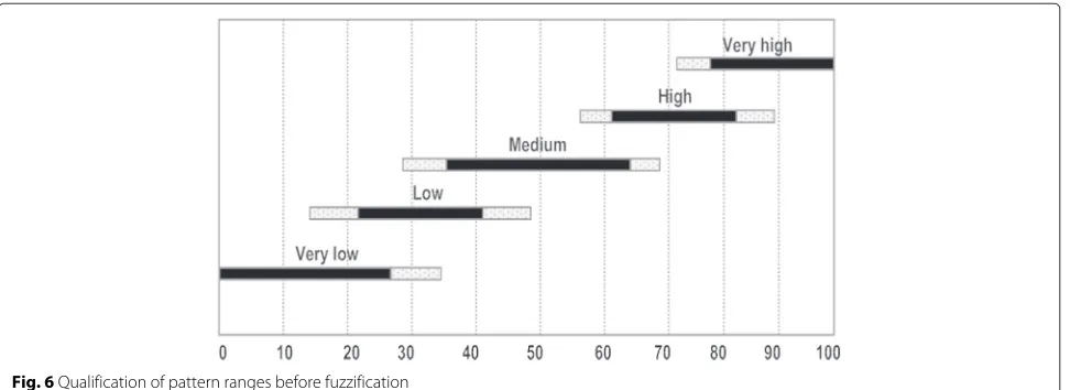
The ranges above reflect observed CPU utilisation ranges under which the performance is relatively stable. Ranges with similar performance are clustered. We now use a qualified representation of the individual range clus-ters. For the CPU processor load, we use five individual labels Very Low, Low, Medium, High and Very High. Thus, for the above mapping, we can map the CPU ranges [16–23] to the Very Low label, [20–33] to Low and [40– 54] and [48–56] to Medium. The labels themselves are suggested by experts and are commonly used in the con-figuration of cloud infrastructure solutions. While this qualification into concept labels is technically not neces-sary, these labels help to visualise and communicate the pattern-based prediction to the cloud users.

Figure 6 shows the qualified patterns. For each label, the black bar denotes the variation of the means of each of the pattern value ranges as given by the experts, e.g., the means of [40–54] and [48–56] for the Medium label. The light grey bars denote the overall variation of ranges for each label.

The qualified categorisation will in the next step be used to define fuzzy membership functions that fuzzify the infrastructure input captured in the patterns.

Defining membership functions

Infrastructure monitoring tools measure the input val-ues for the prediction solution (CPU, storage, network) as infrastructure parameters and performance as service-level data). Their conversion to fuzzy values is realized by MFs. In this section, we show how to derive appropriate IT2 MFs based on the data extracted from the infrastruc-ture and service monitoring logs. We follow the guidelines in [20] in order to construct the functions. To simplify the investigation, we focus on CPU load and performance only.

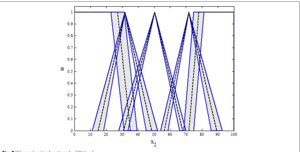
As illustrated in Fig. 5, we used triangular or trapezoidal MFs to represent different CPU load ranges:

• For each normalized CPU range

[CPUmin∼CPUmax], we define one type-2 MF as in

Fig. 7 for five ranges.

• We order these and label them accordingly, e.g., with VL to VH labels representing Very Low to Low, Medium, High and Very High CPU loads.

Letaandbbe the mean values of the interval end-points CPUminandCPUmaxof the labelled ranges with standard deviationsσaandσb, respectively (see Fig. 6). For instance, for the Low, Medium and High label, the corresponding triangular T1 MF is then constructed by connecting leftl, middlemand rightras follows:

l=(a−σa, 0),m=((a+b)/2, 1),r=(b+σb, 0) (30)

Accordingly, for Very Low and Very High processor load ranges that border 0 or 100 % on the normalized scale, the associated trapezoidal MFs can be constructed by connecting points as follows:

(a−σa, 0),(a, 1)(n, 1),(b+σb, 0) (31)

The labels above refer to utilisation rates of resources, with a maximum value being 100. So, irrespective of the

Fig. 7IT2 membership functions for CPU load

concrete system, the labels are assigned to normalised utilisation ranges.

As indicated by the standard deviations in Fig. 6, there are uncertainties associated with the ends and the loca-tions of the MFs. As an example, a triangular T1 MF might be defined follows:

l=(a−0.3×σs, 0) m=((a+b)/2, 1) r=(b+0.4×σb, 0)

(32)

These uncertainties cannot be captured by T1 fuzzy MFs. In IT2 MFs on the other hand, the footprint of uncer-tainty (FOU) can be captured by the upper and lower MFs (UMF and LMF) for each range, see Fig. 8. A blurring parameter 0≤α≤1 can determine the FOU (see Fig. 6).

Here, we useα=0.5. Parameterα=0 reduces IT2 MFs to a T1 MFs, while parameterα = 1 results in fuzzy sets with the widest possible FOUs.

The fuzzy prediction process

After constructing the IT2 fuzzy sets with the MFs and the set of rules for the infrastructure load patterns, the prediction can then start to determine service quality esti-mations. The fuzzy prediction technique proceeds in a number of steps as follows (which we will explain in more detail afterwards):

1. The inputs comprising the workload are first fuzzified.

2. Then, the fuzzified input activates an inference mechanism to produce output IT2 FSs.

3. Decisions made through the inference mechanism are represented in the form of fuzzy values, which cannot be directly used as prediction results. The outputs are then processed by a type-reducer, which combines the output sets and subsequently calculates the center-of-set.

4. The type-reduced FSs are T1 fuzzy sets that need to be defuzzified in the last step to determine the predicted quality valueq.

5. This valueq is then passed back to the user as the predicted quality.

In the first step, we must specify how the numeric inputs ui∈Uifor the CPU utilisation rates are converted to fuzzy sets (a process that called “fuzzification” [18]) so that they can be used by the FLS. Here, we use singletons:

μR˜1 =

1 x=ui

0 otherwise (33)

For the defuzzification step, we use the construct of a centroid [21]. The centroid of a IT2 FSR˜ is the union of the centroids of all its embedded T1 fuzzy setsRe:

C_R˜ ≡ ∀Re

c(Re)=

cl

_˜

R,cr

_˜

R (34)

For the type-reducing step we use the center-of-sets construct [36]. The center-of-set (cos) type reduction is calculated as follows:

Ycos=

fl_∈Fl_,yl_∈C

˜

Gl

N

l=1fl×y1 N

l=1fl

=y_l,yr

(35)

where fl ∈ Fl is the firing degree of mapping rule l andyl ∈ C_G˜l is the centroid of the IT2 FSG˜l. The

cen-troidscl(R˜),cr(R˜) andyl,yr are calculated using the KM algorithm from [21].

Fuzzy reasoning for quality prediction

Our quality mappings that encode the SWPs are in a multi-input single-output format. Because the log records of different services may not be similar, many patterns may be conflicting, i.e., we might have rule mappings with the same antecedent, but different consequent values. In this step, mappings with the same if-part are combined into a single rule. For each mapping in the patterns retrieved from the logs, we get the following for a sample ruleR1:

IF x1is F1l

and . . . and xpis Fpl

,

THEN

y is y(tlu)

(36)

wheretl_u is the index for the result. In order to combine these conflicting mappings, we used the average of all the responses for each mapping and use this as the centroid of the mapping consequent. Note, that the mapping con-sequents are IT2 FSs. However, when the type reduction is used, these IT2 FSs are replaced by their centroids. This means that we represent them as intervalsyn_,yn_{or crisp} values whenyn=yn. This leads to rules with the following form for an arbitrary ruleRl_:

IF the CPU workload (x1) isF˜i1, AND the network load (x2) isG˜i2, AND the storage utilisation (x3) isH˜i3, THEN qiis the predicted value.

whereCis the value of associated consequent, i.e., here a quality value for performance inms, andwl_uis the weight associated with theu-th consequent of the lth mapping. Therefore, eachqican be computed.

In a concrete example, we now illustrate the details of the prediction process. Assume that the normalized val-ues regarding the three input parameters are x1 = 40, x2 = 50 and x3 = 55, respectively – see the solid lines for the workload in Fig. 9 as a sample factor. For x1 = 40, two IT2 FSs for the processor workload rangesF2 = LowandF2 = Mediumwith the degrees [0.3797, 0.5954] and [0.3844, 0.5434] are fired1. Similarly, forx2 = 50, three IT2 FSs for the performance rangesG3=Medium, G4 = Slow, andG5 = Very Slowwith the firing degrees [0, 0.1749], [0.9377, 0.9568] and [0, 0.2212] are fired. For x3 = 55 similar values would emerge. Intuitively, the lower and upper values of the intervals can be computed by finding the y-intercept of the solid lines in the figure, respectively, with the LMF and the UMF of the crossed FSs. As a result, six pattern mappings might result that are fired (here a sample is given):

M8:(F2,G3,H1),M9:(F2,G4,H4), M10:(F2,G5,H4),M13:(F3,G3,H2), M14:(F3,G4,H1),M15:(F3,G5,H2)

(37)

The firing intervals are computed using the meet opera-tion [17]. For instance, the firing interval associated to the patternM9for the CPU attribute is:

m9=μ_M˜9 2(

x₁)⊗μ_G˜9 4(

x₂)=0.3797×0.9377=0.3560

(38)

The output can be obtained using the center-of-set:

Y_l(40, 50, 55)=

yl(40, 50, 55),yr(40, 50, 55)

= [0.9296, 1.1809]

(39)

The defuzzified output can be calculated as follows:

Y(40, 50, 55)= 0.9296+1.1809

2 =1.0553 (40)

Thus, we can finally calculate the predicted quality Y(x1,x2,x3)for all the possible normalized values of the input infrastructure parameters (i.e., x1 ∈[0, 100], x2 ∈ [0, 100],x3∈[0, 100] for CPU, storage and network).

Evaluation

Fig. 9IT2 MFs of for CPU workload ranges

about concerns such as correctness or completeness. We have implemented an experimental test environment to evaluate the accuracy, efficiency and robustness of the solution in the context of uncertainty and dynamic pro-cessing needs.

Implementation architecture and evaluation settings

The implementation of the prediction and configuration technique covers different parts – off-line and on-line components:

• The pattern determination and the construction of the patterns-quality matrix is done off-line based on monitoring logs. The matrix is needed for dynamic configuration and can be updated as required in the cloud system. For the prediction, the accuracy is central. As the construction is off-line, performance overhead for the cloud environment is, as we will demonstrate, negligible.

• The actual prediction through accessing the matrix is done in a dynamic cloud setting as part of a scaling engine that combines prediction and configuration. Here the acceptable performance overhead for the prediction needs to be demonstrated.

• Uncertainties and noise are additional problems that arise in heterogeneous, cross-organisational cloud architectures. Robustness in the presence of these challenges needs to be demonstrated.

For both the accuracy and performance concern, we use a standard prediction solution, collaborative filter-ing (CF) as the benchmark, which is widely used and analysed in terms of these properties, cf. [11, 12] or

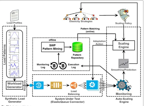
[5, 6]. We have implemented a simulation environ-ment with a workload generator to evaluate accuracy of the prediction approach and the performance of the prediction-based configuration. Test data is derived from sources such as [22] where quality metrics (response time, throughput) are collected for 5825 Web services with 339 users. We selected 100 application services from three different categories, each category either sensitive to data size, network throughput or CPU utilization. Figure 10 describes the testbed with the monitoring and SWP extraction solution for Web services. The primary concern is the accuracy of the pattern extraction and pattern-based prediction of performance for deployed services. Furthermore, as dynamic reconfiguration, i.e., auto-scaling, is an aim, also performance needs to be looked at.

Fig. 10Evaluation architecture

response time for different service types and Figs. 7 and 8 show infrastructure concerns such as CPU and stor-age aspects. In that particular case, 4,100 test runs were conducted, using a 3-service application with between 25 and 200 clients requesting services. Azure CSF telemetry was used to obtain monitoring data. This data was then looked at to identify our workload patterns(CPU, Storage, Network)→Performance.

Cloud application workload patterns

A number of different application workload patterns are described in the literature [8, 13]. These include static, periodic, one-in-a-lifetime, unpredictable, continuously changing as in [8], or slowly varying, quickly varying, dual phase, steep tri-phase, large variation and big spike [13]. We need to make sure that this experimental evalu-ation does indeed cover the applicevalu-ation workload pattern in order to guarantee general applicability. We followed [13] and induced these six patterns in our experiments. Based on the successful pattern coverage, we can conclude that the technique is applicable for a range of the most common situations.

We have implemented our prediction mechanism in dif-ferent platforms. Work we described in [13] deals with how to implement this in an auto-scaling solution such as Amazon AWS where Amazon-monitored workload and performance auto-scaling metrics are considered together with a prediction of anticipated behaviour to configure the compute capabilities.

Accuracy

Reliable performance guarantees based on configuration parameters is the key aim – real performance needs to match the expected or promised one for the provider to fulfill the SLA obligations. Accuracy in virtualisation environments is specifically challenging [24] due to resource contentions because of the layered architecture, shared resources and distribution.

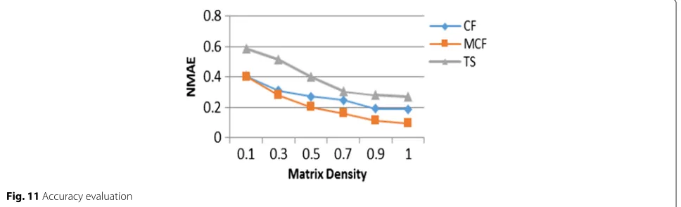
Consequently, we use NMAE (the Normalized Mean Absolute Error) instead of the MAE. The smaller the NMAE, the more accurate is the prediction. We compare our solution with similar methods based on traditional prediction methods in terms of matrix density. This covers different situations from situations where little is known about the services (density is low) and situations where there is a reliable base of historic data for pattern extrac-tion and predicextrac-tion (high density).

In earlier work, we included average-based predications and classical collaborative filtering (CF) in a comparison with our own hybrid method (MCF) of matrix-based matching and collaborative filtering [7]. The NMAE of k = 15 andk = 18 (higher or lowerksare not interest-ing as lower values are statistically not significant and higher ones only show a stabilisation of the trend) shows an accuracy improvement for our solution compared to standard prediction techniques, even without utility function and exponential smoothing, see Fig. 11. For this evaluation here, we also include time series (TS) into the comparison. For the evaluation, we considered some noisy data which cannot be in any pattern. We also removed invocation data and then predicted it using the CF, MCF and also the TS time series method from [25].

We can observe that an increase of the dataset size improves the accuracy significantly. In all cases, our MCF approach outperforms the other ones by resulting in less prediction errors.

Efficiency overhead (runtime)

For automated service management in the context of cloud auto-configuration and auto-scaling we need suf-ficient performance of the extraction and matching approach itself. To be tested in this context are the perfor-mance of three components:

1. SWP Extraction from Logs (Matrix Determination) 2. Configuration-Pattern Matching (Existing Patterns) 3. Collaborative Filtering (Non-Existing Patterns)

For cases 1 and 2, we determined 150 workload patterns from 2400 usage recordings. We tested the algorithm on a range of different datasets extracted from a number of documented benchmarks and test cases. Com-pared to other work based on the TS and CF solutions, the matrix for collaborative computation is reduced from 2400∗100 to 150∗100, which reduces execution time significantly by the factor 16. For case 3, only when a matched pat-tern provides no information for a target service, the calculation for collaboration prediction is required, see Fig. 12, where we compare prediction performance with (MCF) as described in Sections ‘Workload patterns’ and ‘Quality pattern-driven configuration determination’ (using Algorithms 1 and 2) and without (CF) the pattern-based matrix utilisation.

Robustness against noise and uncertainty

Exponential smoothing causes noise and results in some unavoidable errors. We need to demonstrate that our pre-diction solution is resilient against input noises, one of which is the estimation error through smoothing.

We experimentally evaluated the robustness against noise. We observed that the worst estimation error happens for large variation and quickly varying patterns and is less than 10 % of the actual workload. Based on this, we injected a white noise to the input measurement data (i.e.,x1) with an amplitude of 10 %. We ran RMSE (root-mean-square error – measure of the differences between values predicted by a model or an estimator and the values actually observed) measurements for each levels of blurring, and for each measurement, we used 10,000 data items as input. We used different blurring values. Two observations emerged:

• Firstly, the error of control output produced by the prediction technique is less than 0.1 for the blurring levels.

• Secondly, the error of control output is decreasing when we configured the technique with a higher blurring.

Fig. 12Performance evaluation

A higher blurring as part of the smoothing leads to a bigger FOU in the uncertainty management, where FOU is a representative for the supporting levels of uncertainty. Therefore, the designer should make a choice in terms of the level of uncertainty that is acceptable. Note that in some circumstances an overly wide FOU results in a performance degradation. However, we can state that these observations provide enough evidence that robust-ness against input noise is maintained. Using IT2 FLS in the uncertainty management actually alleviates here the impact of noise.

Threats to validity

Some threats to the validity of the observations here exist. The usefulness of the approach relies on the quality of the workload patterns. While the existence of the pat-terns can be guaranteed by simply defining the individual ranges in the broadest possible way, thus resulting in some over-arching default patterns, their usefulness will only emerge if they denote sufficiently narrow ranges to allow the resources to be utilised in an equally narrow band. For instance, a band of 60–80 % is aimed at for processor loads.

While this has emerged to be possible for traditional software services that are computationally intensive or are typical text and static content-driven applications, multi-media type applications for instance with different net-work consumption patterns require more investigation.

Summary of evaluation

Thus, to conclude the evaluation, the computational effort for the dynamic prediction is decreased to a large extent due to the already partially filled matrix. As already explained, the performance of the pattern extraction and

matrix construction (DBSCAN based clustering and col-laborative filtering) can be computationally expensive, but can be done offline and only the matrix-based access (as demonstrated in the performance figure above) impacts on the runtime overhead for the configuration. How-ever, as the results show, our methods overhead increases only slowly even if the data size increases substantially. Consequently, the solution in this setting is no more intru-sive than a reactive rule-based scalability solution such as Amazon AWS Auto Scaling that would also follow our proposed architecture.

We specifically looked at the accuracy and robustness of the solution. The accuracy of the core solution based on the matrix is better than a traditional collaborative fil-tering approach. However, in cloud environments, other concerns needed to be addressed in addition. In order to address uncertainty due to different and possible incom-plete and unreliable log data, we added smoothing and fuzzification. We have demonstrated that these features improve the robustness against external influence factors.

Related work

QoS-based service selection in general has been widely covered. There are three main categories of prediction-based approaches for selection.

• The first one covers statistical and other

mathematical methods, which are often adopted for simplicity [1–3, 26, 27]. Others, e.g., in the context of performance modeling use mathematical models such as queues.

of SLA requirements and the environment and cannot customise prediction for users.

• The third category is based on collaborative filtering [11, 12, 30], which is a widely adopted

recommendation method [31–33], e.g., [32] summarizes the application of collaborative filtering in different types of media recommendation. Here, we combine collaborative filtering with service workload patterns, user requirements and SLA obligations and preferences. This considers different user preferences and makes prediction personalized, while maintaining good performance results.

To demonstrate that our solution is an advancement compared to existing work on prediction accuracy, we had singled out two approaches for categories 1 and 3 for the evaluation above.

General prediction approaches

Some works integrate user preferences and user charac-teristics into QoS prediction [5, 11, 12, 30], e.g. [11, 12] propose prediction algorithms based on collaborative fil-tering. They calculate the similarity between users by their usage data and predict QoS based on user similarity. This method avoids the influence of the environment factor on prediction. However, even the same user will have different QoS experiences over time depending on the configuration of the execution environment or will work with different input data. Current work generally does not consider user requirements. Another current limitation of current solutions is low efficiency as we demonstrated. Our work in [13] is a direction based on fuzzy logic to take user scalability preferences into account for a cloud setting.

In [7, 34], pattern approaches are proposed. Srinivas [34] suggests pattern-based management for cloud con-figuration management, but without a detailed solution. Zhang et al. [7] is about bottom-up QoS prediction for standard service-based architectures, while in this paper QoS requirements are used to predict suitable workload-oriented configurations taking specifically cloud concerns into consideration. We added additionally exponential smoothing and utility functions and the cost analysis here, but draw on some evaluation results from [7] in compari-son to standard statistical methods.

Cloud quality prediction and scalability

Various model-based predictive approaches are in use for cloud quality and resource management, including machine learning techniques for clustering, fuzzy cluster-ing, Kalman filters, or low band filters, used for model updates which are then used for optimization and inte-grate with controllers Supporting cloud service manage-ment can automatically scale the infrastructure to meet

the user/SLA-specified performance requirements, even when multiple user applications are running concurrently. Jamshidi et al. [13] deal with multi-user requirements as part of an uncertainty management approach, which is based on prediction as only exponent smoothing. Ghandi et al. [35] also leverage application level metrics and resource usage metrics to accurately scale infrastructure. They use Kalman filtering to automatically learn changing system parameters and to proactively scale the infrastruc-ture, but have less of a performance gain than through patterns in our solution. Another work in this direc-tion is [36], where the soludirec-tion aims to automatically adapt to unpredicted conditions by dynamically updating a Kriging behaviour model. These deal with uncertainty concerns that we have excluded. However, an integra-tion of both direcintegra-tions would be beneficial in the cloud. These approaches can add the uncertainty management solutions required.

Uncertainty management in clouds

Uncertainty is a common problem, particularly in open multi-layered and distributed environments such as the cloud applications. In [13], fuzzy logic is used to deal with auto-scaling in cloud infrastructures. We have adopted some of the principles here, but applied them to qual-ity prediction here rather than resource allocation there. A similar fuzzy controller for resource management has been suggested in [37] based on adaptive output amplifi-cation and flexible rule selection. However, this solution is based on T1 FLS and does not address uncertainty.

The proposed method in this paper takes full account of user requirements (reflected in SLA obligations for the provider), the network and computational factors. It abstracts the service workload pattern to keep the service QoS steady. When user/SLA requirements are known, prediction-base configuration can be done based on matched patterns. This approach is efficient and reduces the computational overhead.

Conclusions