Williams

GIS ANALYSIS OF HISTORICAL MAPS: A CASE STUDY FROM

AN 1885 SURVEY OF THE CONGAREE RIVER

Thomas M Williams

, David C Shelley

, Bo Song

1

Baruch Institute of Coastal Ecology and Forest Science, Georgetown, SC, USA

2

Old-Growth Bottomland Forest Research and Education Center, Congaree National Park, Hopkins, SC, USA

Abstract. Large floodplain forests, such as the area preserved by Congaree National Park in South

Carolina, are among the most dynamic terrestrial ecosystems known on earth. Flooding and migration of river meanders constantly disturb, create, and erode forest habitats. This provides abundant opportunities for new primary succession. Like many long-term processes, meander evolution is primarily understood from extrapolation of short-term measurements (events or 1-2 year campaigns), decadal-scale rates from comparison of mid- to late 20th century aerial photographs, or millennial-scale trends from geological and geomorphic analysis. There is often a gap in detailed analysis of century-scale geomorphic trends without excessive and expensive radiometric dating techniques. A unique opportunity to examine more than 100 years of channel change on the Congaree River is presented by an 1885 map. This 1:6,000 scale map was prepared from a survey conducted by the US Army to determine the cost of removing snags and rocks impeding steamboat traffic. Using modern GIS techniques maps from that survey were scanned from the National Archives, georeferenced to a modern datum, and used to create a shapefile of the riverbank position in 1885. This project demonstrated problems substantially different from similar efforts georeferencing antique maps, primarily caused by the linear feature and landform changes associated with an alluvial river. A LiDAR based DEM was critical to achieving reasonable river positions and the RMS error was 23 m (75 ft) compared to average bank migration of 155 m (500 ft) over the 114-year period.

Keywords: Congaree National Park, GIS, historical map, old-growth forest, river migration

1

Introduction

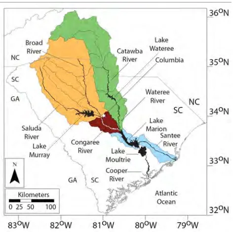
The long-term evolution of river meanders is a fun-damental geomorphic process that is very relevant for understanding bottomland forest ecology of the South At-lantic and Gulf coastal plains (e.g., Hupp, 2000). Changes in the river position over time impact the distribution and development of floodplain soils as well as structure and succession of vegetation communities (e.g., Meitzen, 2006). One prime example of such a system is found on the lower Congaree River in central South Carolina (Figure 1). Over 27,000 acres (10,900 ha) of the flood-plain (including 11,000 acres (4450 ha) of old-growth forest) are preserved in Congaree National Park (Fig-ure 1). Adjacent state and private lands, including the South Carolina Department of Natural Resources Conga-ree Bluffs Heritage Preserve and Poinsett State Park, are also heavily forested. Congaree National Park’s mission is to protect, study, and interpret “the resources, history, story, and wilderness character of the nation’s largest remaining tract of southern old-growth bottomland forest

and its associated ecosystems” (NPS, 2014). A thorough understanding of the planform Congaree River meander evolution at multiple time scales, then, is important for park researchers, managers, partners, and visitors alike.

While spatial patterns of erosion and deposition are not practically predictable in detail at a micro-scale, mi-gration can be understood through a combination of statistical parameters, numerical modeling, and empiri-cal observations at a variety of sempiri-cales. There is a large body of research that has analyzed river movements over the mid- to late 20th century using aerial imagery. Luna Leopold (Leopold et al., 1964; Langbein and Leopold, 1966) examined many meandering rivers utilizing aerial photographs and USGS quadrangle maps. Results of those studies indicate that meander amplitude, wave-length, river width, and radius of curvature all are corre-lated to the mean annual flood discharge. Brice (1974) used aerial photography of over 125 rivers to qualita-tively classify 16 distinct meander geometries related to their evolution. Meanders generally migrate downstream

Copyright©2017 Publisher of theMathematical and Computational Forestry & Natural-Resource Sciences

Figure 1: General location map of the Congaree River within the Santee River watershed in central North and South Carolina. Adapted from Shelley et al. (2012) with USGS HUC data (e.g., USGS, 2015).

but individual meanders may migrate upstream while forming multiple lobes over time. The educational goal of the park can be furthered by determining similarity of form and timing of these processes on the Congaree River within the park.

Staff and research partners at Congaree National Park have analyzed migration rates and trends along the Con-garee River based on historical maps and aerial pho-tographs. Analysis of long-term trends in river migration have been studied based on abandoned channel geome-tries in a floodplain and the classification of distinct river reaches with differing planform geometry controls based on geology and tectonics (Shelley and Cohen, 2010). Shelley et al. (2011) discussed preliminary results of ra-diocarbon analyses to help date cutbank features and abandoned channels on the floodplain; these results, how-ever, which range from about 850 BC to about 1750 AD, are difficult to spatially extrapolate. Aerial photographs from 1938 have also been rectified to 1999 orthophotos and migration since 1938 to determine incremental bank erosion rates in that period (Shelley and Meitzen, 2005; Meitzen and Shelley, 2005). However, between 1938 and 1999, size and frequency of major floods have been differ-ent (smaller) than the period from 1890–1930 (Conrads et al., 2008).

The leap from decadal scale river movements in the late 20th century to long-term river movements over

thousands of years often leaves a gap in detailed, century-scale observations that stretch back into the 18th and 19th centuries. Detailed measurements on these time frames are difficult because aerial photography was not common until the mid-twentieth century. Sediments can be dated using radioisotopes of cesium and carbon, but these studies are time-consuming and expensive. Histori-cal maps certainly exist, but finding maps at sufficient scale and quality for GIS analysis is difficult.

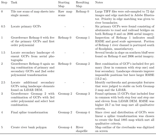
Staff at Congaree National Park recently found refer-ence to an 1885 map of the Congaree River developed as part of a US Army Signal Corps project to clear the river for steamboat traffic. The purpose of the survey was to estimate the cost of dredging a riverboat canal from the Santee River to Columbia (United States Army 1885). The final report of the project included a survey of depths of the Congaree River from the city of Columbia to the confluence with the Wateree River. The map ref-erence was first found in the historical collections of the Caroliniana Library at the University of South Carolina, but the original data and full-size maps were not present. Park staff then contacted the National Archives to obtain full-sized original sheets (Figure 2). The sheets, drafted at 1:6,000 (1” = 500’ or 1 cm = 60 m) scale, stretched to almost 12 feet (3.6 m) when extended. In addition to showing survey points, the maps contained channel depths, cross sections, and several features of interest on the riverbanks. Even with a large format scanner, nine scans were required to produce 400 dpi images of the original map. The goal of this work was to create a GIS layer of the 1885 position of the river channel in a modern map projection, the 1983 North American Datum and the UTM (Zone 17N) projection.

Figure 2: Portion of first map sheet of the 1885 map showing type of information available from the original map. Each map sheet had scale bars and several markers of cardinal directions. Distance along the river, originating at confluence with Wateree River, was marked at each mile. Survey stations (small numbers 1-12 on right bank) and water depths were drafted directly on the map. Cultural features along the river were also noted.

of these transformations, allowing the analyst to concen-trate on the purpose of the transformation rather than the complicated mathematics of geodesy.

Georeferencing of historical maps is generally similar to the procedure done with photographs, but modified to reflect accuracy and precision of the original survey data, as well as the errors introduced by drafting, storage, and rasterization (Balletti, 2006). Cajthaml (2011) separated old maps into 8 categories (a-h) based on three factors; if original map is single or a mosaic of several, if the original scale is known, and if the original projection is known, and made suggestions on the ideal method to

georeference each type. Preservation of maps, as well as structures, from the 16th–19th centuries allowed many projects to be conducted in Europe, especially in Italy (Balletti, 2006; Brigante and Radicioni, 2014; Bitelli et

al., 2009).

Figure 3: Location of the three map sheets of the 1885 map of the Congaree River. Map sheets are indicated by large rectangles while the portions of each sheet formed by individual scans are indicated by dotted line within the rectangles. Ground Control Points listed are indicated by green dots. GCP 1-10 were identified on aerial photography and 10-19 were identified on the LiDAR DEM, with number 10 present on both sources. The base layer shown is the 1999 aerial photographs (SCDNR, 2014a).

of an accurate survey. However, it did not have reference to a datum or projection. With such a map the recom-mended procedure was to locate GCPs on each panel and use an affine (1st order polynomial) transformation to correct the scale and orientation to the modern pro-jection. Once in the correct projection the map sheets can be reassembled with simple edge matching to resolve overlapping regions.

Rather than map sheets of polygons normally used by the references above, the Congaree River map panels only represented the river banks and a few cultural features near the banks (Figure 2). The original map consisted of three drafted sheets, with the third separated into three subsections to accommodate a sharp turn in the river (Figure 3). The sheets were too large to be captured by a single scan. It was obvious that the procedure recom-mended by Cajthaml (2011) was not possible, as most of the scanned sections did not contain any cultural features that could be used as ground control points. In fact, none of the procedures recommended in Cajthaml (2011) could be used because those methods were suited for maps

rep-resenting polygonal features with information along all map edges, allowing mathematical transformations to assure conformity of the map edges. The 1885 map of the river was a linear polygon and contained only neat-lines along the panel edges. The only alternative was to edge match the individual scans and then georeference the entire map.

2

Methods

From a processing standpoint, the ultimate goal was to rectify the map using a spline option that precisely pre-served the known position of all GCPs while transforming the rest of the surrounding image with minimal distortion. However, that goal was attained by an iterative process (Table 1) of examining GCPs and maps produced by global transformations with the fundamental validity of any map transformation in a given area was qualitatively evaluated (or rejected) using three principles:

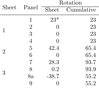
Table 1: Steps used and resulting map products produced during procedure used to create a polygon portraying the banks of the Congaree River in 1885.

Step Task Starting

Map

Resulting Map

Notes

0 Tile raw scans of map sheets into single mosaic.

Raw map scans

Refmap 0 Large TIFF files were sub-sampled to 72 dpi images and edge matched in Adobe Illustra-tor. Priority in edge matching was given to river boundaries.

0.5 Locate primary GCPs - - Six primary GCPs were found consisting of

abutments to road and railroad bridges on both Refmap 0 and on 2006 aerial imagery. 1 Georeference Refmap 0 with five

of the primary GCPs and first order polynomial

Refmap 0 Geomap 1 Inspection of Refmap 1 indicates small RMSE and good scale agreement. Portion of Refmap 1 river channel is portrayed south of floodplain, unsatisfactory.

1.5 Locate secondary landscape el-ement GCPs from aerial pho-tographs

- - Several breaks in slope on southern bluff were found on Refmap 0 and 2006 aerial imagery.

2 Georeference Refmap 0 again us-ing combination of primary and secondary GCPs and 2nd order polynomial transformation

Refmap 0 Geomap 2 Best combination of GCP’s included five pri-mary (four in common with step one) and four secondary. Landscape elements improve impossible positions but have larger RMSE (13.2 m).

2.5 Locate additional secondary GCPs using landscape elements found on LiDAR DEM.

- - Identify earthworks and geomorphic features

that were judged to stable on both Geomap 2 map and the LiDAR.

3 Georeference Geomap 2 with

combination of GCPs with 3rd order polynomial and select best combination.

Geomap 2 Geomap 3 Found optimum 15 GCPs that included four in common with both step four and step one and eleven from LiDAR DEM. RMSE was higher 23.7 m but map met all qualitative criteria.

4 Final spline transformation Geomap 2 Geomap 4 Since river and distribution of GCPs were linear a spline transformation was chosen to create the final 1885 map which met all qualitative criteria.

5 Create river bank polygon Geomap 4 River

shapefile

Map outline of the riverbanks was digitized on screen

(a) the high (>200 ft, or 61 m) bluffs along the south-ern valley margin, (b) historical earthwork features in the lower floodplain, or (c) historical development along the levees of the uppermost river, which is a geomorphi-cally stable, linear bed-rock channel (Shelley and Cohen, 2010).

(2) Second, the 1885 channel position should generally fall in sequence with the known 1938, 1999, and 2006 positions and/or related meander evolution geometries (i.e., Brice, 1974).

(3) Third, the mathematical transformation should minimally (and preferably not) distort the compass roses and printed text nearest the river. Text progressively

farther away from the river may, however, be altered with multiple, higher order transformations.

All GIS processing and analyses were conducted in ArcGIS 10.1 except where noted. The base reference map was prepared from a mosaic of ortho-quarter-quadrangle aerial photographs taken in 2006 (SCDNR, 2014 a, b). These aerial photographs had a resolution of one m (3.3 ft) and were projected in UTM 17 N, NAD83. Inspection of the scans revealed the 1885 map consisted of three drafted sheets. On each sheet were horizontal scale and a separate vertical scale for channel cross-sections. Ori-entation of each sheet was represented by directional arrows in each cardinal direction (Figure 2). On sheets 2 and 3, there were also arrows to indicate the orientation of the previous sheet to indicate the degree of rotation. The third sheets contained three panels to accommodate an 180 degree turn as the channel changed from pre-dominately NE to SE near the confluence of Congaree and Wateree rivers (Figure 3). Each panel of sheet three had two sets of orientation arrows to indicate changes in orientation of the three panels. Cultural features that could be used as ground control points were very sparse on the 1885 map; only a road and two railroad crossings were identified.

Individual scans were resampled to 72 dpi with Adobe Photoshop in order to stay within memory limits of the desktop. Adobe Illustrator was used to orient the raster of each map section to properly align its north arrow (Table 2). Individual sections were then manually edge matched with the adjacent tiles and merged to form a single image. On that single image, six points were identified that corresponded to features found on the aerial photo mosaic: the abutments to bridges on Ger-vais Street; Charlotte, Columbia, and Augusta Railroad (CC&A) Bridge; and South Carolina Railway (SC Ry) Bridge, both now part of Norfolk Southern Railroad. Of these, the CC&A bridge showed the least alterations, while the Gervais Street and SCRy bridges had been rebuilt. Five GCP’s could be used from these three features (Figure 3) for a 1st order polynomial (affine) transformation of the map with a forward RMSE of 6.2 m, producing Geomap 1. The northern abutment of the SCRy bridge had been replaced at a new location and resulted in much higher forward RMSE values when used in any combination with the other five.

The five GCP’s located on the aerial photographs did span most of the length of the river but there were no points over much of central section the river. The georeferenced map violated the first criterion of a success, as Geomap 1 portrayed the river channel south of the bluff along the southern side of the floodplain. A second group of GCPs were located by identifying landscape elements, primarily small tributary creeks incised into the bluff, that could be identified by the infra-red blue coloration of hardwoods compared to the red colored pines found along most of the bluff. Utilizing these new points nine GCPs

Table 2: Initial rotation of scanned images to orient north arrows and edge match with adjacent image. Rotation in degrees counter- clockwise relative to upstream scan. Panel one is the upstream, northwestern portion of the system near modern day Columbia, SC.

Sheet Panel _SheetRotation_Cumulative

1

1 23* 23

2 0 23

3 0 23

4 0 23

2 5 42.4 65.4

6 0 65.4

3

7 28.3 93.7

8 0.2 93.9

8a -38.7 55.2

9 0 55.2

*Initial rotation for North alignment

(Figure 3) with a 2nd order polynomial transformation produced a map (Geomap 2) with a forward RMSE of 13.3 m.

The inclusion of landform GCPs along the bluff im-proved the qualitative performance but doubled the quan-titative estimate of error on Geomap 2. Also, the distri-bution did not include any GCPs on map sheet 2. To improve the distribution of GCPs we used a LiDAR-based DEM of Richland County, SC, with 18.5 cm (0.61 ft) Root Mean Square Error (RMSE) vertical accuracy and 10 x10‘ (3.05 m) cell size and elevation expressed in US foot (SCDNR, 2015). The LiDAR DEM was further pro-cessed into 25 layer files that applied specific color ramps to two foot (0.61 m) intervals, allowing recognition of rel-ative elevation differences of 0.1 ft (3.05 cm). Additional GCPs were developed from LiDAR ground elevation data (Figure 3). While creek channels are not stable in the long-term, a few batture channels, nested channels inset into older river cutoffs, are at least well-constrained. Like-wise, position of creeks in the southern bluff and points where the bluff and floodplain meet at an acute angle were noted on the map. Seventeen points were initially chosen from the LiDAR DEM and an iterative process of point selection was used to determine a set of fifteen points (ten LiDAR DEM and five aerial photos, Figure 3) that produced both a distribution of points on all three original sheets and minimum positional error (RMSE 23.1 m) using a third order polynomial transformation (Geomap 3).

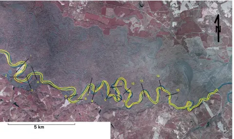
Figure 4: Location of cross sections used to measure rate of meander migration. The base layer shown is the 1999 aerial photographs (SCDNR, 2014a).

GCP precisely, it cannot be used for error estimation. The spline option produces the best fit to the GCP’s points while minimizing distortion of the map far from the points. Following final georeference, the rectified map (Geomap 4) was used to digitize a polygon shapefile of

the 1885 river bank positions

The final shapefile of 1885 channel positions were converted to KML files and exported to Google Earth (Google 2016) for display on 2016 imagery and then compared to boundaries for the 1938 and 1999 channel (e.g. Shelley and Meitzen, 2005; Meitzen and Shelley, 2005). Comparisons were made to examine alignment with the current river and meander evolution with refer-ence to sequrefer-ence types described by Brice (1974). Fifteen sections were selected to represent river sections where meander evolution was clear from evidence of point bar migration in the LiDAR and not influenced by changes in upstream meanders. For each meander, a line was drawn perpendicular to the general river flow direction (Figure 4). Manual estimates of maximum point bar and cut bank migration were made for the 114-year period with the ArcGIS measure tool. Mean annual migration rates and standard deviation were calculated. The cen-ter line of the 1885 channel and the 1999 channel were measured with the ArcGIS 10.1 measure tool along the

same portion of the channel to determine any change in sinuosity during the period.

3

Results and Discussion

Figure 5: Overlay of georeferenced Figure 2 on ortho-photo. Position of GCPs on bridge abutments and errors are displayed in insets. Note georeferenced map scale on left. The base layer shown is the 1999 aerial photographs (SCDNR, 2014a).

Also, most maps contained a number of cultural artifacts (roads, buildings, fields) that had been preserved to the present. In those cases, many GCP’s could be found and georeferencing could be done, more or less, indepen-dent of knowledge of the scale, orientation, or geometric accuracy of the original map.

3.1 Estimating map scale and orientation Geo-referencing of the 1885 map was initially done using five GCPs that could be recognized on the aerial ortho-photos (numbers 1-5 on Figure 3). Three points define a 1st order polynomial transformation (affine Ballati, 2006), which can be used to transform the map scale and orienta-tion. The 1st order polynomial is a global transformation meaning that all pixels, including GCPs, are moved in the georeferenced image. Five GCPs allow an estimate of the error associated with the transformation by estimating the positional error of the transformed GCPs. The first section of Table 4 lists the positional errors of the five GCPs in x and y directions. The RMSE 6.15 m (20 ft) and maximum was 5.45 m (17.9 ft) in the x (east-west) direction and 7.77 m (25.5 ft) in the y (north-south). These errors are represented graphically in Figure 5. As

the affine transformation applies the same mathematical transformations to all pixels in the image, the drafted scale bars on each map sheet (portion of map sheet 1 scale is shown in Figure 2) should accurately represent ground distance.

Table 3: Comparison of on scale bar distances on each of the three map sheets to the distance measured on the 1st order polynomial transformation (affine) using the ArcGIS measure tool. All distances are expressed in feet on the scale bar.

Scale Distance 100 ft 200 ft 300 ft 400 ft 500 ft 1,000 ft 2,000 ft 6,000 ft

30.5 m 61 m 91.5 m 122 m 152.4 m 304.9 m 609.8 m 1,829.3 m

Map Sheet 1 101 ft 198 ft 316 ft 412 ft 529 ft 1,052 ft 2,110 ft 6,232 ft

30.8 m 60.4 m 96.3 m 125.6 m 161.3 m 320.6 m 643.1 m 1,899.5 m

Map Sheet 2 106 ft 197 ft 318 ft 414 ft 519 ft 1,012 ft 2,018 ft 6,550 ft

32.3 m 60.1 m 96.9 m 126.2 m 158.2 m 308.5 m 615.2 m 1,996.5 m

Map Sheet 3 94 ft 185 ft 282 ft 390 ft 492 ft 991 ft 1,981 ft 5,941 ft

28.6 m 56.4 m 86 m 118.9 m 150 m 302 m 603.8 m 1,810.8 m

Table 4: Ground control points used for three phases of georeferencing. Source refers to source of coordinate data either Ortho quarter-quad Aerial Photos (OAP) or LiDAR based DEM. Individual error estimates are presented for each GCP used in production of georeferenced maps with 1st, 2nd, and 3rd order transformations described in the methods section.

GCP Source Geomap 1 Geomap 1 Geomap 2 Geomap 2 Geomap 3 Geomap 3

X error, m Y error m X error m Y error m X error m Y error m

1 AP -0.02 0.13 -0.20 -11.66 34.04 31.66

2 AP -4.89 3.05 0.10 -3.05 4.28 3.66

3 AP -2.01 -5.43 0.28 -6.29 -4.25 -4.05

4 AP 5.45 -5.51 -11.69 -14.47

5 AP 1.47 7.77 -0.36 8.93 11.35 14.51

6 AP 0.17 10.89

7 AP 4.43 5.76

8 AP -4.39 -3.85

9 AP 0.39 -23.60

10 Both -0.32 22.90 -2.40 -2.41

11 LiDAR DEM -17.92 -17.14

12 LiDAR DEM -9.80 -3.48

13 LiDAR DEM -13.89 -15.02

14 LiDAR DEM 44.53 -10.16

15 LiDAR DEM -40.08 20.00

16 LiDAR DEM 7.98 3.28

17 LiDAR DEM -6.63 -9.68

18 LiDAR DEM 1.93 -1.21

19 LiDAR DEM 2.54 4.15

RMSE (m) 6.15 13.13 23.67

3.2 Removing problems identified in first effort The two scans of map sheet 2 could not be matched as precisely as the others. One could match the river banks and one neat line or the directional arrows, but not both. The river bank was chosen as most critical when the scans were mosaiced. The problem caused by this mismatch is also seen easily in Figure 6. The river channel is mapped as flowing south of the present bluff. The mapped position A should be close to the position

A’ to portray this section of the channel correctly. Point A in Figure 6 was similar to several other points where the river was near the bluff and a stream valley could be identified. However, aerial view of a southeastern forested floodplain does not resemble features noted by surveyors traveling along the river over a hundred years ago.

Figure 6: Initial georeferenced map near GCP 10 in Figure 3 showing problem of impossible river position well to south of high bluff. Note complete directional arrows on left but distorted one on right where the two sheets were edge matched by using the river banks as most critical junction. Point A on map indicated a small valley on the bluff which is located somewhere near point A’ on the photograph. The base layer shown is the 1999 aerial photographs (SCDNR, 2014a).

choosing and deleting potential GCPs among these land-scape elements, as well as the original six cultural features a final group of nine GCPs were chosen that produced a 2nd order polynomial rectification with an increased RMSE error of 13.1 m ( Table 4). The final distribution of GCPs did not include any on map sheet 2 (Figure 3). Another source of GCPs was obtained from a Richland County LiDAR mapping mission that produced a DEM of the floodplain.

The 1885 map had a large number of notations on the location of particular features of the ground surface. Although most did not refer to permanent features, there were several that referred to features on the bluff and on the floodplain that could be expected to still exist. Locating these features on the LiDAR surface allowed GCPs to be added to sections of the map that had been scanned as individual images. A major benefit in this analysis was the ability to create repetitive layers of the DEM dataset that displayed small relative changes in soil elevation. Although the absolute accuracy of the elevation data was over 18 cm (0.6 ft), the elevation attribute was a continuous variable that could be sepa-rated into relative classes as small as 0.1 ft (3 cm). Color could then be used to identify abandoned point bar and channel structures across the flood plain.

Seventeen additional GCP were added from the LiDAR DEM. With the addition of more GCPs, the errors of individual GCPs on a 1st order transformation became more than 100 m (330 ft) indicating either poor points

or a problem in orientation of some of the scan bound-aries. Orientation errors could be overcome with the use of a non-linear transformation. Usually a 2nd order polynomial transformation has been used to transform historical maps as a 3rd order tends to distort edges of the map (Balleti 2006). The Congaree River map was an exception to this generality since the only area of interest was near the river, where the GCPs were located. A 3rd order polynomial allowed greater freedom to correct orientation errors and, on this map, distortion away from the river affected edges which generally only contained written notes that were not critical to the task.

A 3rd order polynomial transformation is also a global transformation allowing evaluation of the errors associ-ated with each GCP. These error estimates could be used to evaluate the usefulness of each GCP. Locating points on the LiDAR involved a great deal of subjective ‘expert’ opinion as to permanence of old channel features, but an objective error estimate could be used to eliminate mistakes. The final 15 GCPs were located as depicted in Figure 3 and results of the 3rd order polynomial trans-formation. The 3rd order polynomial transformation (Geomap 3) met all of our criteria for a successful georef-erence of the 1885 map. The fifteen GCPs were evenly distributed with four on each map sheets one and two and six on the multiple sections of map sheet three. They also represented a minimum RMSE of 23.7 m (77.5 ft). The five GCPs used in producing Geomap 1 were also used for Geomap 3 but point 10 was the only landscape element that was consistent on both aerial photographs and LiDAR DEM. This suggests that aerial photointer-pretation is limited to cultural artifacts and landscape elements were better located on the DEM. This is not surprising for the Congaree National Park since most of the park is a closed canopy floodplain forest that has been undisturbed for decades.

The spline transformation differs from the polynomial transformations by being a local and exact transforma-tion. It reproduces the GCPs in their exact location and transforms the map by interpolating between them. Like an inverse distance interpolation, areas distant from GCPs are little changed in the transformation. By geo-referencing the map with the spline transformation the map is changed to pass through the exact position of the GCPs. As most of the GCPs were linearly distributed along the river channel one could argue that the spline transformation presents the best approximation of the position of the river in 1885.

Figure 7: Portion of valley downstream from GCP 14 (Figure 3) that demonstrates appearance of river position overlays for 1885, 1938, and 1999 on both 2016 Google Earth photo and LiDAR DEM. The base layer shown is the 2016 Google Earth imagery (Google 2016).

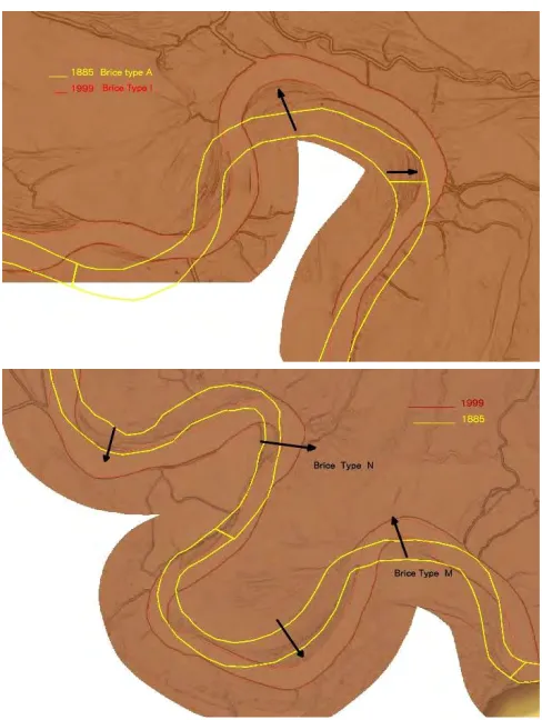
relatively intermediate between the 1885 and 1999 posi-tions. In a few instances within the convoluted meander on the right side of Figure 7 a small point bar is evident between the 1999 position and the 2016 Google image. These point bars are also in positions that seem to show the greatest rate of movement between 1885 and 1999. The general meander evolution also conforms to chan-nel forms and elevation described by Brice (1974). Two such instances are portrayed in Figure 8. To distinguish the subtle slopes of the flood plain, the LiDAR DEM is portrayed as a continuous color ramp from yellow (high) to brown (low) while slopes determined from the DEM are portrayed as semitransparent values of light to dark with steepest slopes dark. In this way the characteristic ridges of point bar deposition appear as a series of dark bands. In Figure 8A, the simple meander, Brice (1974) termed type A, forms secondary loops on both up-valley and down-valley limbs that move outward to form a more complex symmetrical double loop, Brice termed Type I. In Figure 8B, the channel has formed numerous complex asymmetrical loops with a Brice Type N loop moving down valley, while downstream a Type M loop moves up valley providing opportunity for a meander cut off in the future. Baring such cutoffs this trend to increasing meander complexity increases river sinuosity, that was measured between the 1885 and 1999 channels. The 1885 channel was 36,069 meters (22.4 miles) along the park border, from upstream of GCP 10 to GCP1, while the 1999 channel was 38,769 meters (24.1 miles) between those points, resulting in a change in sinuosity from 1.88 to 2.01 for the period. That increase occurred despite

a meander cutoff where the 1885 channel was 1,300 m (4265 ft) long in 1885 but only 200 m (656 ft) in 1999.

Figure 8: A.(Top) Example of a simple meander loop becoming more complex as it changes from a simple Brice Type A to the more complex Brice Type I where secondary loops form on the up valley and down -valley legs of the simple meander. B.(Bottom) Complex meanders where the up–valley meander is forming a type N loop that is moving down valley while the down-valley meander is forming a type M loop that is moving up valley. Slides portray elevation as a gradient from brown to yellow (notice bluff in lower right of B) that is overlaid by a semi-transparent slope that varies from light for mild slopes to dark for steeper slopes. This display allows low gradient floodplain features to be easily seen. The repeated ridges of point bar sedimentation are seen as a series of dark curves. The base layer shown is from SCDNR (2015).

width is similar to that over 100 years ago while the sinuosity has increased over that period.

Table 5: Initial analysis of maximum lateral migration of point bars and cut banks of 15 meander loops on the Congaree River SC from 1885 until 1999. All values were measured perpendicular to the general flow of the river at that point. Distances were measured in direction of meander migration, which in some cases was up valley.

Point bar Cutbank

Cross section Distance (m) Rate (m/yr) Distance (m) Rate (m/yr)

1 119.0 1.14 123.0 1.18

2 85.0 0.82 69.0 0.66

3 217.0 2.09 171.0 1.64

4 127.0 1.22 110.0 1.06

5 88.0 0.85 136.0 1.31

6 57.0 0.55 53.0 0.51

7 141.0 1.36 185.0 1.78

8 136.0 1.31 164.0 1.58

9 160.0 1.54 168.0 1.62

10 330.0 3.17 341.0 3.28

11 98.0 0.94 130.0 1.25

12 235.0 2.26 249.0 2.39

13 175.0 1.68 150.0 1.44

14 197.0 1.89 180.0 1.73

15 138.0 1.33 145.0 1.39

Mean 153.5 1.48 158.3 1.52

Std. Dev. 69.8 0.67 69.3 0.67

4

Conclusion

River meandering has a profound effect on the distribu-tion of soils within an alluvial floodplain. Over geologic time the river erodes and deposits sediments across the entire floodplain. However, meander migration has only been measured on time scales of several thousand years by isotope analysis or over the last several decades using aerial photographic coverage. GIS analysis of a 19th cen-tury survey has shown meander evolution, over a hundred years, to be similar patterns other rivers outlined in Brice (1974). Rate of both point bar and cut bank migration were similar, averaging near 1.5 m/yr for the 114-year period and there was a small increase in the sinuosity of the river despite one meander cutoff occurring during the period.

The historical map of the Congaree River revealed that georeferencing of alluvial river maps produced problems different from those found with other historical maps. The most important difference was in the portrayal of the landscape in the original map. The map was essentially a single linear polygon with little information about

location of points distant from the river. There was little data that could be used to edge match the multiple images of portions of the map. A problem that was common to others working on dynamic alluvial rivers was the general lack of control points that were stable over time. One great advantage was the quality of the original survey and drafting of the map. An affine (1st order polynomial) transformation resulted in the drafted scale to be within 5% of the actual distances represented. It is likely that had the entire map been contained on a single scan it could have been georeferenced to the modern datum with less than a 5% error. The RMS errors of the 3rd order polynomial transformation were about 1/5 the overall average meander movement and 1/3 of the standard deviation of those values.

By far the most important factor allowing the comple-tion of the georeferencing task was the availability of a LiDAR based high resolution Digital Elevation Model. By portraying the subtle slopes of the floodplain, the DEM could be used to determine the position of former channel structures across the floodplain. A combination of judgment about which structures might be permanent over 100 years, and the numerical evaluation of agree-ment of the geometry of those points, we were able find a group of additional GCPs that could be used to produce a consistent georeference of the 1885 channel. By using a both a 3rd order polynomial and a spline we could make the best estimate of the 1885 river position and an estimate of the error inherent in the GCP positions. The spline transformation of those GCPs then allowed development of a map that can be used to portray both the qualitative aspects of meander evolution and to make quantitative estimates of erosion and deposition over the last century.

Acknowledgments

This study was done in partnership with staff at the Congaree National Park who supplied the original digital images of the 1885 map and 1938, and 1999 river position shapefiles. Other data was obtained from the South Carolina, Department of Natural Resources, GIS data Clearing House. The original LiDAR data was produced by a partnership of the U.S. Geological Survey and the South Carolina Department of Natural Resources.

References

Balletti, C. 2006. Georefernce in the analysis of geometric content of early maps. e-Perimetron 1:32-39.

Brice, J.C. 1974. Evolution of meander loops. Geological Society of America Bulletin 85(4): 581–586.

Brigante, R. and Radicioni, F. 2014. Georeferencing of historical maps: GIS technology for urban analysis. Geographica Technica 9(1): 10-19.

Brovelli, M.A., and Minghim, M. 2012. Georeferencing old maps: a polynomial based approach for Como historical cadastres. e-Perimetron 7(3):97-110.

Burrough, P. A., and. McDonnell, R.A. 1998. Principles of Geographical Information Systems, Oxford Univer-sity Press, Toronto.

Cajthaml, J. 2011. Methods of georeferencing old maps on the example of Czech early maps. In Raus, A., ed., Proceedings of the 25th International Carto-graphic Conference, Paris, France, July 3-8, ICACI Paper C0-314, http://icaci.org/files/documents/ICC

proceedings/ICC2011

Conrads, P.A., Feaster, T.D., and Harrelson, L.G. 2008. Analyzing the Effects of the Saluda Dam on the Surface - Water Hydrology of the Congaree National Park Floodplain, South Carolina. Proceedings of the 2008 South Carolina Water Resources Conference, October 14-15, 2008 Charleston, SC.

DeMers, M. N. 2008. Fundamentals of Geographic In-formation Systems, 4th. ed., John Wiley and Sons, Toronto.

Google. 2016. Google Earth version 7.1.8.3036, Google Inc. Mountain View, California.

Hupp, C.F. 2000. Hydrology, geomorphology, and vege-tation of coastal plain rivers in the southeastern USA. Hydrological Processes 14:(16-17): 2991-3010.

Huxhold, W.E. 1991. An Introduction to Urban Geo-graphic Information Systems, Oxford University Press, New York.

Kennedy, M. 2006. Introducing Geographic Information Systems with ArcGIS, John Wiley and Sons, Hoboken, New Jersey.

Langbein, W. B., and Leopold, L. B. 1966. River meanders—Theory of minimum variances: Physio-graphic and hydraulic studies of rivers. USGS Pro-fessional Paper 422-H, US Government Printing Office, Washington, DC, 21 pp.

Leopold, L.B., Wolman, M.G., and Miller, J.P. 1964. Flu-vial processes in geomorphology. Freeman, San Fran-cisco, CA, 522 pp.

Meitzen, K. 2006. Development, Disturbance, and Main-tenance: Process-pattern relationships in riparian en-vironments, Congaree River, Congaree National Park South Carolina [MS Thesis]. Columbia, SC, University of South Carolina Department of Geography, 206 pp.

Meitzen, K., and Shelley, D.C. 2005. Channel planform change on the Congaree River: 1820-2001 [abs.]: Amer-ican Association of Geographers Annual Conference, Denver, CO, April 5-9.

Murphy. P.C., Guralnick, R.P., Glaubitz, R., Neufeld, D., and Ryan, J.A. 2004. Georeferncing of museum collections: A review of problems and automated tools, and the methodology developed by the Mountain and Plains Spatio-Temporal Database-Infomatics Initiative (Mapstedi) Phytoinfomatics 3:1-29.

NPS. 2014. Foundation Document: Congaree Na-tional Park, South Carolina. United States De-partment of the Interior, Washington, DC, 80 pp. https://www.nps.gov/cong/learn/management/upload /CONG FD SP.pdf

SCDNR. 2014a. South Carolina Department

of Natural Resources, GIS Data

Clearing-house, Richland and Calhoun County Map

data, 1999. Orth-quarter Quads. Available at http://www.dnr.sc.gov/GIS/gisdownload.html Accessed on Feb. 26, 2016.

SCDNR. 2014b. South Carolina Department

of Natural Resources, GIS Data

Clearing-house, Richland and Calhoun County Map

data, 2006. Orth-quarter Quads. Available at http://www.dnr.sc.gov/GIS/gisdownload.html Accessed on Feb. 26, 2016.

SCDNR. 2015. South Carolina Department of Natural Re-sources, GIS Data Clearinghouse, LIDAR data. Avail-able at http://www.dnr.sc.gov/GIS/lidarstatus.html. Accessed on Feb 26, 2016.

Shelley, D.C., and Cohen, A.D. 2010, GIS analysis of geologic constraints on the planform geometry of the Congaree River, South Carolina. South Carolina Ge-ology, v. 47, South Carolina Department of Natural Resources Geological Survey, Columbia, SC., p. 19-31.

Shelley, D.C., and Meitzen, K. 2005. Preliminary assess-ment of near-channel floodplain developassess-ment, Conga-ree National Park, South Carolina [abs.]: Final Pro-gram and Abstracts, Society of Wetland Scientists 26th Annual Meeting, p. 48.

development of floodplain landscapes at Congaree Na-tional Park [abs.]. Joint conference of the Southern Appalachian Mountains, the Piedmont-South Atlantic Coast, South Florida-Caribbean, and Gulf Coast Co-operative Ecosystem Studies Units, St. Petersburg, FL, October 25-27.

Shelley, D.C., Werts, S. Dvoracek, D., Armstrong, W. 2012. Bluff to bluff: A field guide to floodplain geology and geomorphology of the Lower Congaree River Valley, South Carolina in Eppes, M.C., and Bartholomew, M.J., eds., From the Blue Ridge to the Coastal Plain: Field Excursions in the Southeastern United States. Geological Society of America Field Guides, v. 29, p.

67-92, doi: 10.1130/2012.0029(02)

United States Army. 1885. Appendix M16: Letters re-garding the 1884-1885 Survey of the Congaree River, South Carolina in United States Army, Annual Report of the Chief of Engineers to the Secretary of War for the Year 1885, Part II. 49th Congress, 1st Session, United States House of Representatives Executive Document 1, part 2, vol. 2. Washington, D.C., United States Government Printing Office, p. 1140-1145.