Using Geostatistics to Estimate the
Variability of Autocorrelated Processes
Sueli Aparecida Mingoti
Department of Statistics, Federal University of Minas Gerais (UFMG), Belo Horizonte, MG, Brazil
E-mail: [email protected]
Otaviano Francisco Neves
Federal University of Minas Gerais (UFMG), Belo Horizonte, MG, Brazil
Abstract
Statistical quality control is used to detect changes in the parameters values of the process which usually are estimated under the assumption of independence of the sampling units with respect to the quality characteristic. However, this is questionable for many processes. The main objective of this paper is to present estimators for the variance of autocorrelated processes by using Geostatistics methodology. With this new procedure the usual Shewhart’s control charts still can be used to monitor the quality of the process. A Monte Carlo simulation study showed that the proposed estimators have good performance.
Keywords: variability, autocorrelation, geostatistics, semivariogram, shewhart’s control charts
Introduction
the randomness of the normal distribution and not due the fact that some modification of the process parameters had occurred. Under the normality assumption the control limits for the average of the process are given by the following equations:
UCL = µ + k ; CL = µ; LCL = µ – k (1)
where µ and σ are the average and the standard deviation of X, respectively and k is the distance of the control limits to the central line expressed in units of standard deviation.
In practice the values of µ and σ are estimated from samples of the process, when it is just under the effect of "common" or "random" causes. Let X1, X2, ..., Xn be the observed values of a random sample of the process. Then the parameter µ is estimated by the sample mean X and the parameter σ is estimated by the standard deviation (s) or the moving sample range (σ^
AM) defined respectively as
where (2)
^
σAM = , where and AMi = |Xi – Xi – 1| (3)
The variance of the process (σ2) is estimated by the square of the estimators (2) and
(3), respectively.
These classical estimation procedures are based on the assumption of independence among the sample units of the process with respect to the quality characteristic X being measured. As mentioned in Alwan and Roberts (1995) this assumption is very questionable especially for chemical processes (Zhang, 1998). With the advances of the technology, processes can be sampled at higher rates which often leads to autocorrelated data. When the estimators (2) or (3) are used to estimate the standard deviaton σ of an autocorrelated process then the chance of "false alarms" or not detecting the "out of control" condition may increase because the calculated control limits will be shorter or wider than the true limits of the process. According to Zhang (1998) and Box and Luceno (1997) positive correlation occurs more frequently in practical situations.
distribution. The possible changes that could happen in the average of the process would be reflected in the behavior of the residuals (Box and Luceno, 1997). Although very interesting, this alternative demands the right identification of the ARIMA model and the calculation of the residual for each new collected sample. Another alternative is to monitor the process by using the EWMA (Exponentially Weighted Moving Average) charts proposed iniatially by Roberts (1959) and discussed by Montgomery and Mastrangelo (1991), Hunter (1998, 1986) among others. Basically the statistical EWMA model is defined as
Zt = lXt + (1 – l) Zt –1 (4)
where 0<l<1 is a constant which needs to be determined by the user and Xt is the value of the quality characteristic X observed for the sample t, t = 1,2,…,n. By using the model (4) the series of the one step forecasts errors is obtained and Shewhart’s control charts are then applied to the series of errors which theoretically should be uncorrelated. The choice of the constant l in (4) is discussed in Crowder (1989), Lucas and Saccucci (1990), Box and Luceno (1997) among others. Basically, it is chosen to minimize the sum of squares of the one step forecasts prediction errors. Hunter (1998) claimed that the EWMA control chart is simpler to implement and can be an efficient tool to be used in companies daily routine. Another approach proposed by Krieger, Champ and Alwan (1992) and Alwan and Alwan (1994) is to use multivariate control such as Hotelling’s T2 chart or multivariate
CUSUM chart to treat observations of an autocorrelated univariate process. This is done by forming a multivariate vector of a moving window of observations from the process. In this approach it is necessary to choose the time delay between samples in such way that the constructed vectors are almost uncorrelated. Apley and Tsung (2002) modified this idea allowing correlation between samples.
The main purpose of this paper is to introduce an automatic and simpler form to monitor the process in the presence of correlation. The alternative we will propose does not depend upon the identification and adjustment of ARIMA models as well as the calculation of one step prediction errors. The idea is to use Geostatistics methodology (Cressie, 1993) to estimate the variance and the standard deviation of the process. The quality of the process is then monitored by the usual Shewhart’s charts applied to original characteristic X of interest by replacing the classical standard deviation estimator in the Shewhart’ control charts for a geostatistical estimator of σ. The correction of the charts due to presence of the correlation is automatically incorporated in the control limits UCL and LCL. The results of a simulation study comparing the geostatistical with the classical estimators will be presented.
Discussing the Effects of the Correlation: ARIMA Models
generated by an auto regressive process (AR) where s2 is the square of s in (2). To see this
consider the AR(1) and MA(1) models defined as
Xt = fXt – 1 + at + δ (5)
Xt = at – qat – 1 + µ (6)
where |f| <1, |q| <1, δ and µ are constants and at~N(0,σ2
a) is a white noise series. In
the AR(1) and MA(1) models the first order autocorrelation is given by f = r1 and
r1 = , respectively.
Zhang (1998) had shown that the expectation of the estimator s2 for an autocorrelated
process is given by
ª
¨ (7)
where rh = Corr (Xi, Xi+h). As we can see from (7) if rh > 0, ∀h, then E[s2] will be smaller
than the true value s2. If r
h < 0,∀h, then E[s2] will be larger than σ2. For processes with a
mixture of positive and negative correlation E[s2] could be smalller or larger than the true
value of σ2 and for large sample sizes (7) converges to σ2. For the AR(1) and MA(1) the
expression (7) reduces respectively to:
(8)
(9)
Tables 1 and 2 show the values of C(n, f) and C(n, q) for samples of sizes n = 25, 100,
f ∈[ – 0.9, 0.9] and q ∈[ – 0.9, 0.9]. It can be seen that for AR(1) the bias of s2 is higher
for n = 25 and positive high correlation. For MA(1) model the bias is negligible for both sample sizes and for all values of q.
Geostatistics Methodology
Table 1 – Values of C(n, f) - AR(1).
f n= 25 n = 100
0.90 0.53 0.84
0.80 0.73 0.92
0.70 0.83 0.95
0.60 0.89 0.97
0.50 0.92 0.98
0.40 0.95 0.99
0.30 0.97 0.99
0.20 0.98 1.00
0.10 0.99 1.00
0.00 1.00 1.00
- 0.10 1.01 1.00
- 0.20 1.01 1.00
- 0.30 1.02 1.00
- 0.40 1.02 1.01
- 0.50 1.03 1.01
- 0.60 1.03 1.01
- 0.70 1.03 1.01
- 0.80 1.04 1.01
- 0.90 1.04 1.01
Table 2 – Values of C(n, f) - MA(1).
q r1 n = 25 n = 100
0.90 - 0.50 1.04 1.01
0.80 - 0.49 1.04 1.01
0.70 - 0.47 1.04 1.01
0.60 - 0.44 1.04 1.01
0.50 - 0.40 1.03 1.01
0.40 - 0.34 1.03 1.01
0.30 - 0.28 1.02 1.01
0.20 - 0.19 1.02 1.00
0.10 - 0.10 1.01 1.00
0.00 0.00 1.00 1.00
- 0.10 0.10 0.99 1.00
- 0.20 0.19 0.98 1.00
- 0.30 0.28 0.98 0.99
- 0.40 0.34 0.97 0.99
- 0.50 0.40 0.97 0.99
- 0.60 0.44 0.96 0.99
- 0.70 0.47 0.96 0.99
- 0.80 0.49 0.96 0.99
general references in Geostatistics are Cressie (1993), Journell and Huijbregts (1997), Chilès and Delfiner (1999) and Houlding (2000).
Briefly speaking, suppose we have a random sample of a random variable X collected in many different locations from a certain area. In this case, statistical models are build with the main objective to predict the value of X for locations not in the original sample. These models incorporate the information of the existing relationship among the sample values of X for different locations through a function called semivariogram (or variogram) which plays an important role in the spatial prediction procedure called Kriging (Cressie, 1993). In the Kriging procedure the value of X for a new location with coordinates s0 for example, is predicted based upon the values of X in a neighborhood of s0. Although Geostatistics can be used for locations in ℜd space most of the applications are related to ℜ2. Next we will
introduce the Geostatistics definitions in ℜspace.
Geostatistics in the ℜ Domain: Main Concepts
The sequence of observed values of the quality characteristic X can be treated as a trajectory of a stochastic process {X (t), t ∈ℜ}.The variability of the process can be expressed in terms of the theoretical semivariogram of the process. Two assumptions are necessary: intrinsically stationarity and the isotropy. Shortly, these assumptions are described as follows:
A. Intrinsically Stationarity: The stochastic process {X(t), t∈ℜ} is such that: (i)E [X(t)] = µ, ∀t∈ℜ;
(ii)Var [X(tl) – X (tk)] = 2γ (||tl – tk||), ∀tl≠tk, ∈ℜ,
which means that the process has constant average in ℜ, and for all tl,tk∈ℜ, tl≠tk, the variance of the difference [X (tl) – X (tk)] is a function only of the difference ||tl – tk|| depending on its magnitude and direction. The funcions 2γ (•) and γ(•) are called variogram and semivariogram of the process, respectively.
B. Isotropy: If the variogram 2γ (•) is a function only of the distance among the sample units then the process is said to be isotropic.
source affecting the process. Some common semivariograms models are: spherical, linear, gaussian, exponential and wave (Cressie, 1993). In practice the theoretical semivariogram is estimated by using a sample of the process {X(t), t∈ℜ}.
At this point it is interesting to notice that for intrinsically stationarity and isotropic processes the semivariogram γ (•) can be expressed as
γ(h) = 1/2{Var[X(t + h) – X(t)]} = 1/2{Var[X(t + h)] + Var[X(t)]} – (10)
Cov[X(t), X(t + h)] = σ2 – σ2Corr[X(t), X(t + h)] = σ2(1 – r
h), ∀h
where rh is the correlation between Xi and Xj, |i – j| = h, i ≠ j.When the correlation is
equal to zero the semivariogram of order h is equal to the natural variance σ2 of the process.
By the Eq. (10) it is clear that in order to estimate the variance σ2 it will be enough to have
estimators of the semivariogram γ (•) and the correlation of order h, rh. Therefore, it is
possible to create many alternative estimators for the variance σ2 that automatically will
take into account the correlation of the process. There are many semivariogram estimators for γ (h), called experimental semivariograms (Cressie, 1993) but Matheron’s (1963) classic estimator is the most well known. Given a sample of n observations of the process, denoted by X1, X2, ..., Xn, Matheron’s estimator of γ (h) is defined as
^
γ(h)= , ∀h ∈ T (11)
where Xi is the value of the quality characteristic X for the sample unit i, i = 1, 2,...,
n, T = {1, 2,..., n -1}, (n – h) is the number of pairs (Xi, Xj) such that |i – j| = h, i ≠ j. The
autocorrelation function of order h, rh, is estimated by
(12)
where is the sample mean. The functions (γ (h), rh) are estimated under
the assumption that the process is intrinsically stationary and isotropic which is the same as saying that the process is “under control”. In the next section we present the new estimators for σ2 that will be discussed in this paper.
New Estimators for the Process Variability: Geostatistics Approach
In Mingoti (2000) and Neves (2001) several estimators were proposed to estimate the variance σ2 of autocorrelated processes based on Geostatistics methodology. In this
estimators (2) and (3). They were constructed considering the relation (10) of section 3. All geostatistical estimators are biased but the bias converges to zero for large samples. In all cases an estimate of the standard deviation is obtained by taking the square root of the estimated variance.
The estimator σ^2
1 defined as
^ σ2
1 = (13)
takes into account only the semivariogram and autocorrelation of order 1 and it is very simple to calculate. The estimator σ^2
2 defined as
^ σ2
2 = (14)
takes into account the three first semivariogram and autocorrelation values. It is an option for process which have significant correlations of order higher than 1. The estimator ^σ2
3
introduced by Mingoti and Fidelis (2001) is the average of the M semivariogram values, where
M is a constant in the set {1,2,...,(n – 1)}. In practice M should be chosen in the neigboorhood of [n/2], where [x] denotes the larger integer number less or equal to x, and such that the number of pairs (Xi, Xj) used to estimate γ (h) is higher ou equal to 30. This is the region where the semivariogram is estimated with better precision (Journel and Huijbregts, 1997).
^ σ2
3 = (15)
The estimator σ^2
4 is an extension of the estimator σ^23 and the correction term in the
denominator has the purpose to decrease the bias of the estimator σ^2 3.
^ σ2
4 = (16)
Finally, the estimator σ^2
5 is a modification of σ^24 where M is defined as in σ^23. The
purpose of using more than just 3 semivariogram values to estimate σ2 is to increase the
precision.
^ σ2
5 = (17)
The geostatistical estimators can also be used in situations where the process is monitored by using averages of rational groups. If X1 , X2, ..., Xm represent the average values of m sample groups then formulas (11) and (12) should be applied to the Xk values, k = 1, 2, …, m, to estimate the semivariogram and correlation of order h of the theoretical stochastic process which is generating the Xk average values. The new formulas are defined as
^
γ (h) = , ∀ h ∈T* (18)
¤ ¦§¥ µ¶´ µ¶ ´ ¦§
¥
µ¶ ´ ¦§
¥
¤
n 1 i
2 i
h i i
h m
1 i h
X X
X X X X ˆ
R (19)
where ¤
m
1 i Xi
m 1
X is the global mean, T* = {1, 2, ..., m – 1}, and (m – h) is the
number of pairs (Xi, Xj) such that |i – j| = h, i ≠ j. The Shewhart’s control limits for the average of the process are then given by
UCL = X + kσ^
i; CL = X; LCL = X – k σ^i (20)
where σ^
i, is any geostatistical estimator presented in this section calculated with the
semivariogram and correlation estimates given by Eqs. (18) and (19), i = 1, 2, 3, 4, 5.
Simulation Results
In this section we present the results of a Monte Carlo simulation study performed to evaluate the geostatistical estimators presented in section 4 for the standard deviation of the process. They were also compared to the classical estimator s and the moving sample range σ^
AM defined in section 1. Samples with sizes n = 25, 50 and 100 were generated from
an AR(1) with parameter f ∈ [– 0.9, 0.9] and from an ARMA(1,1) with the parameters (f, q) chosen such that r1∈ [– 0.95, 0.95]. The region of simulation contains models with long
and short, positive and negative, correlation structure. As an illustration, for the AR(1) with f= 0.9 the autocorrelation for h = 7 is equal to 0.478 while for the AR(1) with f= 0.7
the autocorrelation for h = 3 is only 0.34. The choice of AR(1) and ARMA(1,1) was due to the fact that those are the more commom models for autocorrelated processes according to the literature (see Box and Luceno, 1997; Zhang, 1998). All generated processes had the same fixed mean. The white noise was generated from a normal distribution with zero mean and standard deviation σa ranging from 2 to 7. The constant M = [n / 2] was
the AR(1) and ARMA (1,1) considering all simulated cases, are shown in Tables 3 and 4 as a function of the true correlation r1. The respective values of (f, q) are also shown in the Table 4. Table 5 presents the average results as a function of the white noise standard deviation σa. From Tables 3 and 4 it can be seen that in the presence of correlation the geostatistical estimators had better or similar performance than the classical estimators
s and σ^
AM. Among the geostatistical estimators in general, for high negative correlation
the estimator σ^
5 had a better performance; for intermediate negative correlation σ^1 and ^
σ2 had smaller error values (ME, MAE, MSE) and for high positive correlation the estimators ^
σ1 and σ^2 had a better performance. When the correlation is small the average errors of all
the estimators are more similar. For high positive correlation the estimator σ^
3 presented
smaller errors than the classical estimators. Considering that the estimator σ^
3 does not
have any correcting factor for bias this is an interesting result. In general the estimator σ^ 4
presented larger errors than the estimator s but the difference was not very accentuated. In all cases the moving sample range estimator σ^
AM had a very bad performance with larger
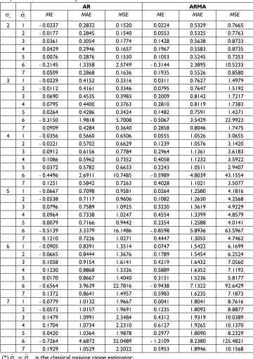
error values especially the MSE. From Table 5 it can be seen that for all the estimators the error values increase as σa increases. The increase rate is much higher for the ARMA than the
AR process. The geostatistical estimator σ^
5 had superior performance for the ARMA process
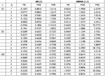
and a good performance for the AR. Table 6 presents the average results as a function of the sample size n. As expected for all the estimators the errors decrease as n increases. In general the errors (ME, MAE, MSE) are larger for ARMA than for AR process. The MSE values for the σ^
AM are intolerable for small and larger sample sizes. By considering the average
results ME, MAE, MSE for all cases presented in Tables 3 and 4 for AR(1) and ARMA(1,1) we can see that the classical standard sample deviation had smaller values only in 2 cases for AR(1) and in 4 cases for ARMA(1,1) compared to the geostatistical estimators.
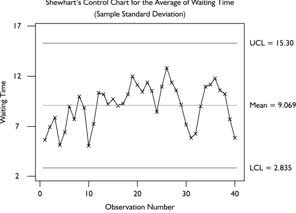
Example of Application
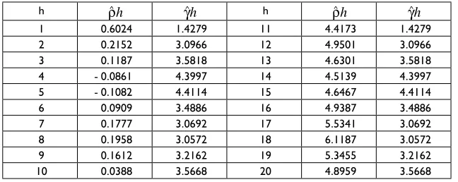
Table 7 presents the observed values of waiting time in line (in minutes) for 40 customers of a laboratory. The autocorrelation and semivariogram estimates for h = 1, 2, …, 20, are presented in Table 8. Table 9 shows the obtained estimates for the standard deviation σ
using all 7 estimators discussed in this paper. As an example, Shewhart’s control charts for the average waiting time using the sample standard deviation s and the geostatistical estimator σ^
1 are presented in Figure 1. As one can see the control limits calculated by
using the estimator σ^
1 are shorter than the limits calculated using the sample standard
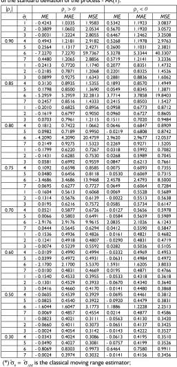
Table 3 – Average results for the geostatistical and classical estimators of the standard deviation of the process - AR(1).
|r1| r1 > 0 r1 < 0
^σ
i ME MAE MSE ME MAE MSE
1 - 0.4243 1.0335 1.9583 0.5342 1.1923 3.0837 2 - 0.3809 1.0602 2.0534 0.5670 1.1920 3.0572 3 - 0.0031 1.2224 2.8055 0.6467 1.2462 3.2508 0.90 4 0.4943 1.2181 2.9182 0.5268 1.1978 2.9763 5 0.2564 1.1317 2.4271 0.2600 1.1031 2.3821 6 - 7.2270 7.2270 59.7367 5.3278 5.3344 40.3307 7 0.4480 1.2065 2.8856 0.5719 1.2141 3.2336 1 - 0.2413 0.7720 1.1740 0.2077 0.8351 1.4732 2 - 0.2185 0.7871 1.2068 0.2201 0.8325 1.4526 3 0.0899 0.9275 1.6343 0.2881 0.8836 1.6062 0.85 4 0.3130 0.8935 1.5355 0.1893 0.8570 1.4949 5 0.1798 0.8500 1.3690 0.0549 0.8345 1.3871 6 - 5.2959 5.2959 32.2813 3.7714 3.7858 19.8403 7 0.2457 0.8516 1.4333 0.2415 0.8503 1.5427 1 - 0.2010 0.6825 0.8956 0.0958 0.6773 0.8712 2 - 0.1619 0.6797 0.9050 0.0960 0.6727 0.8605 3 0.0703 0.7961 1.2115 0.1511 0.7020 0.9484 0.80 4 0.1812 0.7422 1.0662 0.0646 0.6847 0.8909 5 0.0982 0.7189 0.9950 - 0.0219 0.6808 0.8742 6 - 4.2090 4.2090 20.4759 2.9620 2.9677 12.0537 7 0.2149 0.9275 1.5323 0.2269 0.9271 1.5205 1 - 0.1799 0.6220 0.7267 0.0318 0.5992 0.7082 2 - 0.1431 0.6285 0.7530 0.0268 0.5989 0.7045 3 0.0581 0.6992 0.9559 0.0847 0.6213 0.7661 0.75 4 0.1092 0.6598 0.8585 0.0075 0.6093 0.7355 5 0.0480 0.6456 0.8118 - 0.0530 0.6069 0.7315 6 - 3.4686 3.4686 13.9468 2.4578 2.4793 8.5000 7 0.0695 0.6277 0.7727 0.0649 0.6064 0.7284 1 - 0.1604 0.5613 0.6068 0.0069 0.5528 0.5689 2 - 0.1314 0.5676 0.6139 - 0.0022 0.5513 0.5638 3 0.0195 0.6216 0.7572 0.0585 0.5734 0.6147 0.70 4 0.0521 0.5877 0.6726 - 0.0127 0.5656 0.5978 5 0.0066 0.5803 0.6491 - 0.0584 0.5659 0.5989 6 - 2.9176 2.9176 9.9615 2.0835 2.1026 6.1243 7 0.0444 0.5645 0.6294 0.0412 0.5590 0.5847 1 - 0.1536 0.4936 0.4826 - 0.0161 0.4821 0.4682 2 - 0.1241 0.4918 0.4807 - 0.0290 0.4831 0.4719 3 - 0.0074 0.5239 0.5592 0.0282 0.5026 0.5105 0.60 4 - 0.0109 0.4990 0.4994 - 0.0332 0.4969 0.4953 5 - 0.0399 0.4972 0.4931 - 0.0631 0.4984 0.4972 6 - 2.1700 2.1700 5.5370 1.5931 1.6205 3.8033 7 - 0.0100 0.4831 0.4669 0.0195 0.4871 0.4766 1 - 0.1540 0.4533 0.3955 - 0.0533 0.4318 0.3618 2 - 0.1301 0.4529 0.3933 - 0.0670 0.4340 0.3640 3 - 0.0416 0.4660 0.4170 - 0.0141 0.4480 0.3868 0.50 4 - 0.0605 0.4539 0.3929 - 0.0695 0.4461 0.3812 5 - 0.0825 0.4540 0.3922 - 0.0920 0.4479 0.3831 6 - 1.6044 1.6047 3.1773 1.1886 1.2228 2.2513 7 0.0069 0.4857 0.4554 0.0214 0.4877 0.4586 1 - 0.0823 0.4021 0.3111 - 0.0563 0.4130 0.3420 2 - 0.0660 0.4011 0.3073 - 0.0651 0.4137 0.3425 3 - 0.0024 0.4054 0.3142 - 0.0143 0.4222 0.3527 0.30 4 - 0.0343 0.4024 0.3086 - 0.0613 0.4195 0.3510 5 - 0.0490 0.4027 0.3081 - 0.0757 0.4199 0.3526 6 - 0.8069 0.8303 0.9973 0.6464 0.7580 0.9911 7 - 0.0024 0.3974 0.3032 - 0.0141 0.4156 0.3456 (*)^σ
6 =
^σ
AM is the classical moving range estimator;
^σ
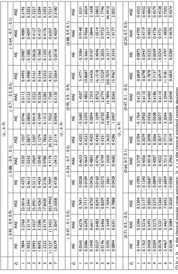
Table 4 – A
verage results for the geostatistical and classical estimators of the standard deviation of the process - ARMA(1,1).
( r1 , f , q )
(- 0.95, - 0.9, 0.9)
(- 0.88, - 0.9, - 0.1)
(- 0.71, - 0.5, 0.5)
(- 0.64, - 0.7, - 0.1)
^ σi
ME MAE MSE ME MAE MSE ME MAE MSE ME MAE MSE 1 1.7894 3.2760 23.0016 0.4372 1.0220 2.1037 - 0.0746 0.5112 0.4993 - 0.0987 0.4085 0.3195 2 1.9032 3.3174 23.5941 0.4613 1.0242 2.0877 - 0.0850 0.5123 0.4980 - 0.1085 0.4097 0.3202 3 2.0993 3.4337 25.0951 0.5513 1.0969 2.3307 - 0.0410 0.5222 0.5161 - 0.0626 0.4127 0.3257 4 1.8692 3.3286 23.4263 0.4424 1.0540 2.1274 - 0.1049 0.5236 0.5166 - 0.1060 0.4157 0.3284 5 1.2222 3.0179 17.8430 0.2196 0.9780 1.7826 - 0.1413 0.5282 0.5252 - 0.1203 0.4176 0.3303 6 11.5237 11.5452 203.9942 4.7097 4.7179 30.7231 1.7022 1.7260 4.3521 0.4791 0.6207 0.7237 7 1.8379 3.3047 23.5058 0.4738 1.0413 2.2114 - 0.0404 0.5130 0.5064 - 0.0518 0.4059 0.3180 ( r1 , f , q )
(- 0.47, - 0.1, 0.5)
(- 0.24, - 0.7, - 0.5)
(0.95, 0.9, - 0.9)
(0.88, 0.9, 0.1)
^ σi
ME MAE MSE ME MAE MSE ME MAE MSE ME MAE MSE 1 0.0545 0.6276 0.7691 0.0028 0.4633 0.4202 - 0.5683 1.4507 5.4771 - 0.3584 0.9148 1.5531 2 0.0386 0.6293 0.7717 - 0.0109 0.4647 0.4233 - 0.5293 2.4852 10.8687 - 0.3661 0.9266 1.6054 3 0.1040 0.6611 0.8750 0.0426 0.4803 0.4502 0.0894 2.7353 13.6426 0.0107 1.0844 2.1658 4 0.0237 0.6483 0.8293 - 0.0160 0.4746 0.4340 1.1699 2.8752 16.1518 0.4046 1.0514 2.0852 5 - 0.0196 0.6466 0.8209 - 0.0373 0.4749 0.4331 0.6720 2.6774 13.5529 0.2025 0.9723 1.7746 6 2.3295 2.3449 7.7694 1.2061 1.2420 2.3625 - 14.7894 14.7894 250.7075 - 6.2217 6.2217 44.4910 7 0.0894 0.6351 0.7888 0.0428 0.4682 0.4286 1.0407 2.8365 15.9467 0.3543 1.0177 2.0021 ( r1 , f , q )
(0.71, 0.5, - 0.5)
(0.64, 0.7, 0.1)
(0.47, 0.1, - 0.5)
(0.24, 0.7, 0.5)
^ σi
ME MAE MSE ME MAE MSE ME MAE MSE ME MAE MSE 1 - 0.1944 0.5284 0.5304 - 0.1093 0.5729 0.5704 - 0.1764 0.6125 0.6839 - 0.0875 0.4705 0.4322 2 - 0.1763 0.5216 0.5177 - 0.1340 0.4056 0.3079 - 0.0950 0.6110 0.6798 - 0.0447 0.4719 0.4432 3 - 0.0458 0.5493 0.5850 - 0.0687 0.4018 0.3098 0.0456 0.6460 0.7878 0.0225 0.4835 0.4842 4 - 0.0209 0.5272 0.5375 - 0.0899 0.4007 0.3066 0.0508 0.6186 0.7137 - 0.0049 0.4736 0.4579 5 - 0.0578 0.5231 0.5260 - 0.1031 0.4022 0.3077 0.0077 0.6110 0.6919 - 0.0254 0.4731 0.4538 6 - 2.4467 2.4467 7.0452 - 0.6859 0.7212 0.7715 - 3.2044 3.2044 11.9181 - 1.4797 1.4820 2.7502 7 - 0.0248 0.5084 0.5020 - 0.0585 0.3963 0.3019 0.0509 0.6040 0.6835 0.0284 0.4676 0.4374 (*) ^σ 6 = ^σ AM
is the classical moving range estimator;
^σ
7
=
s
Table 5 – Average results for the geostatistical and classical estimators of the standard deviation of the process as a function of σa.
AR ARMA
σa ^
σi ME MAE MSE ME MAE MSE
2 1 - 0.0237 0.2832 0.1520 0.0224 0.5329 0.7665
2 - 0.0177 0.2845 0.1540 0.0553 0.5325 0.7763
3 0.0361 0.3054 0.1774 0.1428 0.5638 0.8733
4 0.0429 0.2946 0.1657 0.1967 0.5583 0.8735
5 0.0076 0.2876 0.1530 0.1053 0.5245 0.7253
6 - 0.2145 1.3358 2.5749 - 0.3144 2.3895 10.5233
7 0.0509 0.2868 0.1636 0.1935 0.5526 0.8580
3 1 - 0.0229 0.4152 0.3316 0.0311 0.7627 1.4979
2 - 0.0112 0.4161 0.3346 0.0795 0.7647 1.5192
3 0.0690 0.4535 0.3983 0.2009 0.8142 1.7217
4 0.0795 0.4400 0.3763 0.2810 0.8119 1.7383
5 0.0264 0.4286 0.3424 0.1482 0.7591 1.4371
6 - 0.3150 1.9818 5.7008 - 0.5067 3.5429 22.9923
7 0.0909 0.4284 0.3640 0.2858 0.8046 1.7475
4 1 - 0.0356 0.5660 0.6506 0.0555 1.0526 3.0655
2 - 0.0221 0.5702 0.6629 0.1239 1.0576 3.1420
3 0.0912 0.6156 0.7784 0.2964 1.1361 3.6183
4 0.1086 0.5962 0.7352 0.4058 1.1232 3.5922
5 0.0372 0.5782 0.6633 0.2243 1.0511 2.9407
6 - 0.4496 2.6911 10.7485 - 0.5989 4.8039 43.1554
7 0.1251 0.5842 0.7263 0.4028 1.1021 3.5077
5 1 - 0.0667 0.7098 0.9581 0.0264 1.2580 4.1816
2 - 0.0538 0.7117 0.9606 0.1082 1.2630 4.2568
3 0.0796 0.7589 1.0925 0.3220 1.3619 4.9229
4 0.0964 0.7338 1.0247 0.4554 1.3399 4.8579
5 0.0079 0.7166 0.9442 0.2354 1.2588 4.0141
6 - 0.5139 3.3379 16.1486 - 0.8598 5.8936 63.5967
7 0.1210 0.7226 1.0271 0.4447 1.3055 4.7462
6 1 - 0.0905 0.8391 1.3514 0.0747 1.5422 6.1699
2 - 0.0665 0.8444 1.3676 0.1789 1.5454 6.2524
3 0.1058 0.9154 1.6141 0.4219 1.6432 7.0560
4 0.1230 0.8868 1.5326 0.5889 1.6352 7.1192
5 0.0170 0.8667 1.4040 0.3151 1.5236 5.8177
6 - 0.6564 3.9639 22.7816 - 0.9438 7.1322 92.6429
7 0.1372 0.8641 1.4957 0.5983 1.6235 7.1873
7 1 - 0.0779 1.0132 1.9667 0.0041 1.8041 8.7616
2 - 0.0573 1.0157 1.9691 0.1235 1.8092 8.8877
3 0.1479 1.0991 2.3484 0.4312 1.9319 10.0389
4 0.1704 1.0734 2.2310 0.6127 1.9265 10.1370
5 0.0420 1.0364 1.9878 0.2977 1.8090 8.2329
6 - 0.7264 4.6872 32.0489 - 1.2109 8.2380 125.4821
7 0.1929 1.0529 2.2022 0.5953 1.8946 10.1568
(*) ^σ
6 =
^
σAM is the classical moving range estimator;
^
Table 6 – Average results for the geostatistical and classical estimators of the standard deviation of the process as a function of n (positive correlation).
AR (1) ARMA (1,1)
n ^σ
i ME MAE MSE ME MAE MSE
25 1 - 0.1047 0.8810 1.6116 0.0624 1.4900 6.3739
2 - 0.0777 0.8863 1.6219 0.1732 1.5023 6.5316
3 0.1038 0.9381 1.8308 0.3697 1.5676 7.0518
4 0.1352 0.9040 1.7246 0.5916 1.5669 7.1198
5 0.0002 0.8722 1.5255 0.2512 1.4274 5.4412
6 - 0.3946 3.1806 17.5410 - 0.3650 5.7222 70.7773
7 0.1961 0.9107 1.8032 0.6759 1.5886 7.4756
50 1 - 0.0389 0.6033 0.7235 0.0469 1.1244 3.7361
2 - 0.0277 0.6058 0.7311 0.1222 1.1281 3.7905
3 0.1004 0.6628 0.9067 0.3509 1.2284 4.5496
4 0.1098 0.6456 0.8600 0.4490 1.2188 4.5964
5 0.0396 0.6289 0.7938 0.2705 1.1511 3.8849
6 - 0.4914 2.9513 14.3296 - 0.7816 5.2984 58.1726
7 0.1076 0.6223 0.7957 0.4090 1.1853 4.4118
100 1 - 0.0150 0.4290 0.3702 - 0.0022 0.8619 2.1116
2 - 0.0089 0.4292 0.3715 0.0393 0.8559 2.0950
3 0.0606 0.4731 0.4671 0.1870 0.9295 2.5142
4 0.0654 0.4629 0.4482 0.2296 0.9118 2.4430
5 0.0293 0.4560 0.4281 0.1413 0.8846 2.2578
6 - 0.5520 2.8670 13.1310 - 1.0707 4.9793 50.2466
7 0.0552 0.4365 0.3906 0.1753 0.8676 2.2144
(*) ^σ
6 =
^
σAM is the classical moving range estimator; ^
σ7 = s is the classical standard sample deviation.
Table 7 – Customers waiting time data.
Customer Waiting time Customer Waiting time
1 5.60 21 10.44
2 6.94 22 11.37
3 7.85 23 10.52
4 5.10 24 8.44
5 6.40 25 10.93
6 9.00 26 12.79
7 7.70 27 11.38
8 9.96 28 10.59
9 8.82 29 9.12
10 5.04 30 7.18
11 7.25 31 5.84
12 10.32 32 6.27
13 10.16 33 8.99
14 9.20 34 10.96
15 9.70 35 11.18
16 9.05 36 11.80
17 9.27 37 10.61
18 10.20 38 10.21
19 11.96 39 7.67
Figure 1 – Shewhart’s control charts for the average of customers waiting time.
Shewhart’s Control Chart for the Average of Waiting Time (Sample Standard Deviation)
Observation Number
0 10 20 30 40
W
aiting Time
17
12
7
2
UCL = 15.30
Mean = 9.069
LCL = 2.835
Shewhart’s Control Chart for the Average of Waiting Time (Geostatistical Estimator 1)
Observation Number
0 10 20 30 40
W
aiting Time
UCL = 14.75
Mean = 9.069
LCL = 3.384 15
10
Concluding Remarks
In this paper we presented new estimators for the variance and standard deviation of autocorrelated processes based upon the concepts of Geostatistics methodology. In the presence of correlation this estimation procedure is very appealing because it allows the user to keep monitoring the quality of the process by using the usual Shewhart’s control charts. It was shown that in general the geostatistical estimators ^σ
1 and ^
σ2 had better or similar performance than the classical standard sample deviation s in all simulated cases. In the cases where the classical standard sample deviation s presents better performance than the geostatistical estimators ^σ
3, ^
σ4, ^σ
5, the difference in terms of average error values
were not to large. For high negative correlation the estimator ^σ
5 was the best and for all
the other cases the estimators ^σ 1 and
^
σ2 had better performance. This paper also shows that the classical moving sample range estimator should not be used to estimate the standard deviation of autocorrelated processes. This fact was also pointed out by Mingoti and Neves (2003).
Table 8 – Semivariogram and autocorrelation estimates waiting time - queuing system example.
h r^h γ^h h r^h γ^h
1 0.6024 1.4279 11 4.4173 1.4279
2 0.2152 3.0966 12 4.9501 3.0966
3 0.1187 3.5818 13 4.6301 3.5818
4 - 0.0861 4.3997 14 4.5139 4.3997
5 - 0.1082 4.4114 15 4.6467 4.4114
6 0.0909 3.4886 16 4.9387 3.4886
7 0.1777 3.0692 17 5.5341 3.0692
8 0.1958 3.0572 18 6.1187 3.0572
9 0.1612 3.2162 19 5.3455 3.2162
10 0.0388 3.5668 20 4.8959 3.5668
Table 9 – Estimates of the standard deviation waiting time example.
Estimator Estimate
Geostatistics 1 1.8950 Geostatistics 2 1.9819 Geostatistics 3 2.0409 Geostatistics 4 2.0433 Geostatistics 5 2.0206
Moving range 1.2513
Acknowlegement
This work was partially supported by the Brazilian Institution CNPq.
References
Alwan, A. J., Alwan, L. C. (1994) “Monitoring Autocorrelated Processes Using Multivariate Quality Control Charts”, Proceedings of the Decision Sciences Institute Annual Meeting, 3, pp. 2106-2108.
Alwan, L. C., Roberts, H. V. (1995) “The Problem of Missplaced Control Limits”, Applied Statistics, JRSS, Series C, Vol 44, No 3, pp. 269-278.
Alwan, L. C., Roberts, H. V. (1989) “Time Series Modelling for Statistical Process Control”, Journal of Business & Economic Statistics, Vol 6, No 1, pp.87-95.
Apley, D.W., Tsung, F. (2002) “ The Autoregressive T2 Chart for Monitoring Univariate
Autocorrelated Processes”, Journal of Quality Technology, Vol 34, No 1, pp. 80-96. Box, G.P., Jenkins, G.M. (1976), Time Series Analysis: Forecasting and Control, Holden
Day, New York.
Box, G. P. Luceno, A. (1997), Statistical Control by Monitoring and Feedback Adjustment. John Wiley & Sons, New York.
Chilès, J. P., Delfiner, P. (1999), Geostatistics: Modelling Spatial Uncertainty, John Wiley & Sons, New York.
Cressie, N. (1993), Statistics for Spatial Data, John Wiley & Sons, New York.
Crowder, S. V. (1989) “Design of Exponentially Weighted Moving Average Schemes”, Journal of Quality Technology, Vol 21, No 3, pp.155-162.
Gy, P. (1998), Sampling for Analytical Purposes, John Wiley & Sons, New York.
Gy, P. (1982), Sampling of Particulate Materials, Elsevier Scientific Publishers, New York. Houlding,S. W. (2000), Practical Geostatistics, Springer Verlag, New York.
Hunter, J. S. (1998) “The Box-Jenkins Manual Bounded Adjustment Chart: Graphical Tool Designed for Use on the Production Floor”, Quality Progress, Vol 31, No 8, pp.129-137. Hunter, J. S. (1986) “The Exponentially Weighted Moving Average”, Journal of Quality
Technology, Vol 18, No 4, pp. 202-209.
Journel, A. G., Huijbregts, Ch. J. (1997), Mining Geostatistics, Academic Press, New York. Kitanidis, P. K. (1997), Introduction to Geostatistics: Applications to Hydrogeology,
Cambridge University Press, Cambridge.
Krieger, C. A., Champ, C. W., Alwan, L. C. (1992) “ Monitoring an Autocorrelated Process”, Presented at the Pittisburgh Conference on Modelling and Simulation, Pittisburgh, PA. Lucas, J. M., Caccucci, M. S. (1990) “Exponentially Weighted Moving Average Control
Schemes: Properties and Enhancements (with discussion)”, Technometrics, Vol 32, No 1, pp. 1-129.
Mingoti, S. A. (2000), Aplicação de Novas Ferramentas Estatísticas no Monitoramento do Controle de Qualidade de Processos de Produção, Technical Report: CNPq (In Portuguese).
Mingoti, S. A., Neves, O. F. (1999) “A Metodologia de Geoestatística como Alternativa na Análise de Séries Temporais”, Revista Escola de Minas, Vol 52, No.3, pp.182-187 (In Portuguese).
Mingoti, S. A., Fidelis, M. T. (2001) “Aplicando a Geoestatística no Controle Estatístico de Processos”, Revista Produto & Produção, Vol 5, No 2, pp. 55-70 (In Portuguese). Mingoti, S. A., Neves, O. F. (2003) “A Note on the Zhang Omnibus Test for Normality Based
on the Q Statistics”, Journal of Applied Statistics Vol 30, No 3, pp. 335-341.
Montgomery, D. C. (2001), Introduction to Statistical Quality Control, John Wiley & Sons, New York.
Montgomery, D. C, Mastrangelo, C. M. (1991) “Some Statistical Process Control Methods for Autocorrelated Data”, Journal of Quality Technology, Vol 23, No 3, pp.179-193.
Neves, O. F. (2001), Estudo de Novos Estimadores para a Variabilidade de Processos. Master Dissertation. Statistics Department of Federal University of Minas Gerais, Belo Horizonte, Brazil. (In Portuguese).
Ord, J. K., Rees, M. (1979) “Spatial Processes: Recent Developments with Applications to Hydrology”, in Mathematics of Hydrology and Water Resources, Academic Press, London, pp. 95-118.
Roberts, S. W. (1959) “Control Chart Tests Based on Geometric Moving Averages”, Technometrics, Vol 1, No 3, pp. 239-251.
Runger, G. C., T. R. Willemain, T. R. (1995) “Model-Based and Model-Free Control of Autocorrelated Processes”, Journal of Quality Technology, Vol 27, No 4, pp. 283-292. Thiebaux, H. J., M. A. Pedder, M. A. (1987), Spatial Objective Analysis with Applications in
Atmosphere Science, Academic Press, London.
Zhang, N. F. (1998) “Estimating Process Capability Indexes for Autocorrelated Data, Journal of Applied Statistics, Vol 25, No 4, pp. 559-574.
Yeah, T. C. J., Gutjahr, A. L., Jin, M. (1995) “ An Interative Cokriging-Like Technique for Ground- Water Flow Modelling”, Ground Water, Vol 33, No 1, pp. 33-41.
Biography
Sueli Mingoti holds a Ph.D. in Statistics from Iowa State University, Ames, Iowa, USA in 1989 and she is currently an Adjunct Professor at the Department of Statistics of UFMG (Federal University of Minas Gerais), Belo Horizonte, Brazil