Towards an Optimal Separation of Space and Length in Resolution

(1)

www.theoryofcomputing.org

Towards an Optimal Separation of

Space and Length in Resolution

∗

Jakob Nordström

†

Johan Håstad

‡

Received February 16, 2011; Revised March 9, 2013; Published May 27, 2013

Abstract: Most state-of-the-art satisfiability algorithms today are variants of the DPLL procedure augmented with clause learning. The main bottleneck for such algorithms, other than the obvious one of time, is the amount of memory used. In the field of proof complexity, the resources of time and memory correspond to the length and space of resolution proofs. There has been a long line of research trying to understand these proof complexity measures, as well as relating them to the width of proofs, i.e., the size of a largest clause in the proof, which has been shown to be intimately connected with both length and space. While strong results have been proven for length and width, our understanding of space has been quite poor. For instance, it has remained open whether the fact that a formula is provable in short length implies that it is also provable in small space (which is the case for length versus width), or

∗_A_{preliminary version}_{of this paper appeared in the}_{Proceedings of the 40th Annual ACM Symposium on Theory of}

Computing (STOC ’08).

†_{Part of this work done while at the Massachusetts Institute of Technology supported by the Royal Swedish Academy of} Sciences, the Ericsson Research Foundation, the Sweden-America Foundation, the Foundation Olle Engkvist Byggmästare, and the Foundation Blanceflor Boncompagni-Ludovisi, née Bildt. Currently supported by the European Research Council under the European Union’s Seventh Framework Programme (FP7/2007–2013) / ERC grant agreement no 279611 and by Swedish Research Council grants 621-2010-4797 and 621-2012-5645.

‡_{Supported by the European Research Council under the European Union’s Seventh Framework Programme}

(FP7/2007–2013) / ERC grant agreement no 226203.

ACM Classification:F.4.1, F.1.3, I.2.3

AMS Classification:68Q05, 68Q15, 68Q17, 68T15

(2)

whether these measures are unrelated in the sense that short proofs can be arbitrarily complex with respect to space.

In this paper, we present some evidence indicating that the latter case should hold and provide a roadmap for how such an optimal separation result could be obtained. We do so by proving a tight bound ofΘ(

√

n)on the space needed for so-called pebbling contradictions over pyramid graphs of sizen. This yields the first polynomial lower bound on space that is not a consequence of a corresponding lower bound on width, as well as an improvement of the weak separation of space and width (Nordström, STOC 2006) from logarithmic to polynomial.

1 Introduction

Ever since the fundamentalNP-completeness result of Cook [24], the problem of deciding whether a given propositional logic formula in conjunctive normal form (CNF) is satisfiable or not has been on center stage in Theoretical Computer Science. In more recent years,SATISFIABILITYhas gone from a problem of mainly theoretical interest to a practical approach for solving applied problems. Although all known Boolean satisfiability solvers (SAT solvers) have exponential running time in the worst case, enormous progress in performance has led to satisfiability algorithms becoming a standard tool for solving a large number of real-world problems such as hardware and software verification, experiment design, circuit diagnosis, and scheduling.

A rather surprising aspect of this development is that the most successful SAT solvers to date are still variants of the resolution-based Davis-Putnam-Logemann-Loveland (DPLL) procedure [28,29] augmented withclause learning[7,46]. For instance, the great majority of the best algorithms in recent rounds of the international SAT competitions [58] fit this description. DPLL procedures perform a recursive backtrack search in the space of partial truth value assignments. The idea behind clause learning is that at each failure (backtrack) point in the search tree, the system derives a reason for the inconsistency in the form of a new clause and then adds this clause to the original CNF formula (“learning” the clause). This can save a lot of work later on in the proof search, when some other partial truth value assignment fails for similar reasons. The second main bottleneck for this approach, in addition to the obvious one of time, is the amount of memory used by the algorithms. Since there is only a limited amount of space, all clauses cannot be stored. The difficulty lies in obtaining a highly selective and efficient clause caching scheme that nevertheless keeps the clauses needed. Thus, understanding time and memory requirements for clause learning algorithms, and how these requirements are related to one another, is a question of great practical importance. We refer to, e.g., [41,45] for a more detailed discussion SAT solving with examples of applications.

The study of proof complexity originated with the seminal paper of Cook and Reckhow [26]. In its most general form, a proof system for a languageLis a predicateP(x,π), computable in time polynomial

in|x|and|π|, such that for allx∈Lthere is a stringπ (aproof) for whichP(x,π) =1, whereas for any

x6∈Lit holds for all stringsπ thatP(x,π) =0. A proof system is said to be polynomially bounded if for

everyx∈Lthere is a proofπxof size at most polynomial in|x|. Apropositional proof systemis a proof system for the language of tautologies in propositional logic.

From a theoretical point of view, one important motivation for proof complexity is the intimate connection with the question ofPversusNP. SinceNPis exactly the set of languages with polynomially bounded proof systems, and sinceTAUTOLOGYcan be seen to be the dual problem ofSATISFIABILITY, we have the famous theorem of [26] thatNP=co-NPif and only if there exists a polynomially bounded propositional proof system. Hence, if it could be shown that there are no such proof systems,P6=NP would follow as a corollary sincePis closed under complement. One way of approaching this distant goal is to study stronger and stronger proof systems and try to prove superpolynomial lower bounds on proof size. However, although great progress has been made in the last couple of decades for a variety of proof systems, it seems that we are still very far from fully understanding the reasoning power of even quite simple ones.

(5)

proving tautologies (or, equivalently, testing satisfiability), is an important problem not only in the theory of computation but also in applied research and industry. All automated theorem provers, regardless of whether they actually produce a written proof or not, explicitly or implicitly define a system in which proofs are searched for and rules which determine what proofs in this system look like. Proof complexity analyzes what it takes to simply write down and verify the proofs that such an automated theorem prover might find, ignoring the computational effort needed to actually find them. Thus, a lower bound for a proof system tells us that any algorithm, even an optimal (non-deterministic) one making all the right choices, must necessarily use at least the amount of a certain resource specified by this bound. In the other direction, theoretical upper bounds on some proof complexity measure give us hope of finding good proof search algorithms with respect to this measure, provided that we can design algorithms that search for proofs in the system in an efficient manner. For DPLL procedures with clause learning, the time and memory resources used are measured by thelengthandspaceof proofs in the resolution proof system.

The field of proof complexity also has rich connections to cryptography, artificial intelligence and mathematical logic. Some good surveys providing more details are [8,11,59].

1.1 Previous work

Any formula in propositional logic can be converted to a CNF formula that is only linearly larger and is unsatisfiable if and only if the original formula is a tautology. Therefore, any sound and complete system for refuting CNF formulas can be considered as a general propositional proof system.

Perhaps the single most studied proof system in propositional proof complexity,resolution, is such a system that produces proofs of the unsatisfiability of CNF formulas. The resolution proof system appeared in [18] and began to be investigated in connection with automated theorem proving in the 1960s [28,29,56]. Because of its simplicity—there is only one derivation rule—and because all lines in a proof are clauses, this proof system readily lends itself to proof search algorithms.

Being so simple and fundamental, resolution was also a natural target to attack when developing methods for proving lower bounds in proof complexity. In this context, it is more convenient to prove bounds on thelengthof refutations, i. e., the number of clauses, rather than on the total size of refutations. The length and size measure differ by at most a multiplicative factor given by the number of variables and are hence polynomially related. In 1968, Tseitin [61] presented a superpolynomial lower bound on refutation length for a restricted form of resolution, calledregularresolution, but it was not until almost 20 years later that Haken [36] proved the first superpolynomial lower bound for general resolution. This (weakly) exponential lower bound of Haken has later been followed by many other strong results on resolution refutation length for different formula families, e. g., in [10,17,22,23,52,54,55,62].

A second complexity measure for resolution, first made explicit by Galil [33], is thewidth, measured as the maximal size of a clause in the refutation. Ben-Sasson and Wigderson [17] showed that the minimal widthW(F`⊥)of any resolution refutation of ak-CNF formulaFis bounded from above by the minimal refutation lengthL(F` ⊥)by

W(F` ⊥) =OpnlogL(F` ⊥)

, (1.1)

(6)

bound on the total number of distinct clauses of widthw), the result in [17] can be interpreted as saying roughly that there exists a short refutation of thek-CNF formulaFif and only if there exists a (reasonably) narrow refutation ofF. This gives rise to a natural proof search heuristic: to find a short refutation, search for refutations in small width. It was shown in [14] that there are formula families for which this heuristic exponentially outperforms any DPLL procedure regardless of branching function.

The formal study ofspace1in resolution was initiated by Esteban and Torán [31]. Intuitively, the spaceSp(π)of a refutationπ is the maximal number of clauses one needs to keep in memory while

verifying the refutation, and the spaceSp(F ` ⊥)of refutingF is defined as the minimal space of any resolution refutation ofF. A number of upper and lower bounds for refutation space in resolution and other proof systems were subsequently presented in, for example, [2,13,30,32]. Just as for width, the minimum space of refuting a formula can be upper-bounded by the size of the formula. Somewhat unexpectedly, however, it also turned out that the lower bounds on refutation space for several different formula families exactly matched previously known lower bounds on refutation width. Atserias and Dalmau [5] showed that this was not a coincidence, but that the inequality

W(F` ⊥)≤Sp(F` ⊥) +O(1) (1.2) holds for anyk-CNF formulaF, where the (small) constant term depends onk. In [47], the first author proved that the inequality (1.2) is asymptotically strict by exhibiting ak-CNF formula family of size O(n) refutable in widthW(Fn` ⊥) =O(1)but requiring spaceSp(Fn` ⊥) =Θ(logn).

1.2 Questions left open by previous research

Despite all the research that has gone into understanding the resolution proof system, a number of fundamental questions have remained unsolved. We touch briefly on two such questions below, and then discuss a third one, which is the main focus of this paper, in somewhat more detail.

As was mentioned above, equation (1.1) says that short refutation length implies narrow refutation width. Observe, however, that this doesnotmean that there is a refutation that is both short and narrow, since there is no guarantee that the refutations on the left- and right-hand sides of (1.1) are the same one. An intriguing open question is whether small length and width can always be achieved simultaneously, or whether there is a trade-off between these two measures. For the restricted case of so-calledtree-like

resolution it is known that there can be strong trade-offs [12], but the case of the (much more powerful) general resolution proof system has remained open.

A second, analogous problem concerns space and length. Combining equation (1.2) with the observa-tion above that narrow refutaobserva-tions are trivially short, one can immediately conclude that small refutaobserva-tion clause space implies short refutation length. But again, this doesnotimply that any small-space refutation must also be short. In fact, it was shown in [12] that the refutations on the two sides of the inequality (1.2) in general cannot be the same one. An interesting question is whether small space of a refutation implies that it can also be made short, or whether space and length might have to be traded off against one another.

(7)

A third, even more fundamental question is whether short length has any implications for space. Note that for width, rewriting the bound in (1.1) in terms of the number of clauses|Fn|instead of the number of variables tells us that if the width of refutingFnisω p|Fn|log|Fn|, then the length of refutingFnmust be superpolynomial in|Fn|. This is known to be almost tight, since [20] shows that there is ak-CNF formula family{Fn}∞_n=₁that requires widthΩ 3

p |Fn|

but nevertheless can be refuted in length O(|Fn|). Hence, formula families refutable in polynomial length can have somewhat wide minimum-width refutations, but not arbitrarily wide ones.

What does the corresponding relation between length and space look like? The inequality (1.2) tells us that any correlation between length and clause space cannot be tighter than the correlation between length and width, so in particular we get from the previous paragraph thatk-CNF formulas refutable in polynomial length may have at least “somewhat spacious” minimum-space refutations. At the other end of the spectrum, given any resolution refutationπ ofF in lengthLit can be proven using results from [31,39] that the space needed is at most O(L/logL). This gives an upper bound on any possible separation of the two measures. But is there a Ben-Sasson–Wigderson style upper bound on space in terms of length similar to (1.1)? Or are length and space on the contrary unrelated in the sense that there existk-CNF formulasFnwith short refutations but maximal possible refutation space

Sp(Fn` ⊥) =Ω L(Fn` ⊥)/logL(Fn` ⊥)

in terms of length?

We remark that for tree-like resolution, [31] showed that there is a tight correspondence between length and space, exactly as for length versus width. The case for general resolution has been discussed in, e. g., [12,32,60], but there has been no consensus on what the right answer should be. However, these papers identify a plausible formula family for answering the question, namely so-calledpebbling contradictionsdefined in terms of pebble games over directed acyclic graphs.

1.3 Our contribution

The main result in this paper provides an indication that the true answer to the question about the relationship between space and length is more likely to be at the latter extreme, i. e., that the two measures can be separated in the strongest sense possible. More specifically, as a step towards reaching this goal we prove an asymptotically tight bound on the clause space of refuting pebbling contradictions over so-called pyramid graphs.

Theorem 1.1. The clause space of refuting pebbling contradictions over pyramid graphs of height h in resolution grows asΘ(h), provided that the number of variables per vertex in the pebbling contradictions

is at least2.

This theorem yields the first separation of space and length (in the sense of a polynomial lower bound on space for formulas refutable in polynomial length) that is not a consequence of a corresponding lower bound on width, as well as an exponential improvement of the separation of space and width in [47]. Namely, fromTheorem 1.1we easily obtain the following corollary.

Corollary 1.2. For all k≥4, there is a family{Fn}∞_n=₁ of k-CNF formulas of size Θ(n) that can be

refuted in resolution in length L(Fn` ⊥) =O(n)and width W(Fn` ⊥) =O(1)but require clause space

Sp(Fn` ⊥) =Θ( √

(8)

1.4 Subsequent developments

In a joint paper [15] by Ben-Sasson and the first author, the separation inCorollary 1.2has been improved to a clause space lower boundSp(Fn` ⊥) =Ω(n/logn)while still keeping the upper bounds on length

L(Fn`⊥) =O(n)and widthW(Fn`⊥) =O(1). This is essentially optimal up to multiplicative constants (except possibly for a logarithmic factor in the space-width separation). The construction in [15] follows the general roadmap laid out in the current paper, but changes the family of formulas under consideration inTheorem 1.1. The new results are therefore incomparable with those in the current paper in that the techniques used in [15] cannot proveTheorem 1.1, whereas our techniques, although similar, do not extend to the results in [15].

Even considering the progress made in [15], we believe that the results presented in our paper retain independent interest. This is so since our formula families are simpler, and an improvement of our techniques could conceivably yield optimal, tight results up to constantadditiveterms. This, in turn, could possibly be used to settle the question how hard it is to decide the space requirements for refuting a

k-CNF formula. This problem is easily seen to be inPSPACEbut is not known to bePSPACE-complete. Due to the inherent space blow-up between upper and lower bounds in [15], it is hard to envision the results from there being used for similar purposes. We elaborate briefly on this issue inSection 9.

2 Proof overview and paper organization

Since the proof of our main theorem is fairly involved, we start by giving an intuitive, high-level description of the proofs of our results and outlining how this paper is organized.

2.1 Sketch of preliminaries

A resolution refutation of a CNF formula F can be viewed as a sequence of derivation steps on a blackboard. In each step we may write a clause fromF on the blackboard (anaxiomclause), erase a clause from the blackboard or derive some new clause implied by the clauses currently written on the blackboard.2 The refutation ends when we reach the contradictory empty clause. Thelengthof a resolution refutation is the number of clauses in the refutation, thewidthis the size of the largest clause in the refutation, and theclause spaceis the maximum number of clauses on the blackboard simultaneously. We writeL(F` ⊥),W(F` ⊥)andSp(F` ⊥)to denote the minimum length, width and clause space, respectively, of any resolution refutation ofF.

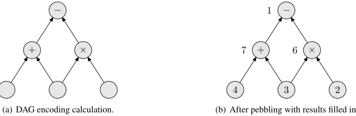
Thepebble gameplayed on a directed acyclic graph (DAG)Gmodels the calculation described byG, where the source vertices contain the input and non-source vertices specify operations on the values of the predecessors (seeFigure 1). Placing a pebble on a vertexvcorresponds to storing in memory the partial result of the calculation described by the subgraph rooted atv. Removing a pebble fromvcorresponds to deleting the partial result ofvfrom memory. Apebblingof a DAGGis a sequence of moves starting with an empty graphGwithout pebbles and ending with all vertices inGempty except for a pebble on the (unique) sink vertex. Thecostof a pebbling is the maximal number of pebbles used simultaneously

(9)

−

+ ×

(a) DAG encoding calculation.

−

+ ×

4 3 2

1

7 6

(b) After pebbling with results filled in.

Figure 1: Example of modelling calculation as pebbling of DAG.

at any point in time during the pebbling. Thepebbling priceof a DAGGis the minimum cost of any pebbling, i. e., the minimum number of memory registers required to perform the complete calculation described byG.

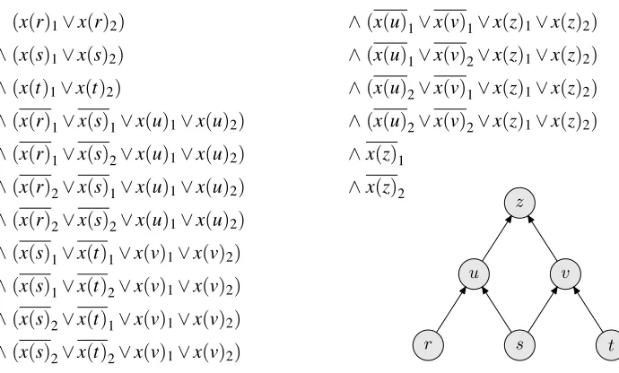
The pebble game on a DAGGcan be encoded as an unsatisfiable CNF formulaPebd_G, a so-called

pebbling contradictionof degreed. SeeFigure 2for a small example. Very briefly, pebbling contradictions are constructed as follows:

• Associatedvariablesx(v)1, . . . ,x(v)dwith each vertexv(inFigure 2we haved=2).

• Specify that all sources have at least one true variable, for example, the clausex(r)1∨x(r)2for the

vertexrinFigure 2.

• Add clauses saying that truth propagates from predecessors to successors. For instance, for the vertexuwith predecessorsrands, clauses 4–7 inFigure 2are the CNF encoding of the implication (x(r)1∨x(r)2)∧(x(s)1∨x(s)2)→(x(u)1∨x(u)2).

• To get a contradiction, conclude the formula withx(z)₁∧ · · · ∧x(z)_dwherezis the sink of the DAG. We will need the observation from [14] that a pebbling contradiction of degree d over a graph with

nvertices can be refuted by resolution in length O d2·nand width O(d).

2.2 Proof idea for pebbling contradictions space bound

(10)

(x(r)1∨x(r)2) ∧(x(u)1∨x(v)1∨x(z)1∨x(z)2)

∧(x(s)1∨x(s)2) ∧(x(u)₁∨x(v)₂∨x(z)1∨x(z)2)

∧(x(t)1∨x(t)2) ∧(x(u)2∨x(v)1∨x(z)1∨x(z)2)

∧(x(r)₁∨x(s)₁∨x(u)1∨x(u)2) ∧(x(u)2∨x(v)2∨x(z)1∨x(z)2)

∧(x(r)₁∨x(s)₂∨x(u)1∨x(u)2) ∧x(z)₁

∧(x(r)₂∨x(s)₁∨x(u)1∨x(u)2) ∧x(z)2

∧(x(r)₂∨x(s)₂∨x(u)1∨x(u)2)

∧(x(s)₁∨x(t)₁∨x(v)1∨x(v)2)

∧(x(s)₁∨x(t)₂∨x(v)1∨x(v)2)

∧(x(s)₂∨x(t)₁∨x(v)1∨x(v)2)

∧(x(s)₂∨x(t)₂∨x(v)1∨x(v)2)

z

u v

r s t

Figure 2: The pebbling contradictionPeb2_Π2 for the pyramid graphΠ2of height 2.

More specifically, what we would like to do is to establish a connection between resolution refutations of pebbling contradictions on the one hand, and the so-calledblack-white pebble game[27] modelling the non-deterministic computations described by the underlying graphs on the other. Our intuition is that the resolution proof system should have to conform to the combinatorics of the pebble game in the sense that from any resolution refutation of a pebbling contradictionPebd_Gwe should be able to extract a pebbling of the DAGG. Our goal is to prove a lower bound on the resolution refutation space of pebbling contradictions reasoning along the following lines:

1. First, find a way of interpreting sets of clauses currently “on the blackboard” in a refutation of the formulaPebd_Gin terms of black and white pebbles on the vertices of the DAGG.

2. Then, prove that this interpretation captures the pebble game in the following sense: for any resolu-tion refutaresolu-tion ofPebd_G, looking at consecutive sets of clauses on the blackboard and considering the corresponding sets of pebbles in the graph we get a black-white pebbling ofGin accordance with the rules of the pebble game.

3. Finally, show that the interpretation also captures clause space in the sense that if the content of the blackboard corresponds toNpebbles on the graph, then there must be at leastNclauses on the blackboard.

Combining the above with known lower bounds on the pebbling price ofG, this would imply a lower bound on the refutation space of pebbling contradictions and a separation from length and width. For clarity, let us spell out what the formal argument of this would look like.

(11)

this graph was chosen with high pebbling price. But this means that at timet, there are a lot of clauses on the blackboard. Since this holds for any resolution refutation, the refutation space ofPebd_Gmust be large. The separation result now follows from the fact that pebbling contradictions are known to be refutable in linear length and constant width ifdis fixed.

Unfortunately, we cannot quite get this idea to work. In the next subsection, we describe the modifications that we are forced to make and show how we can make the bits and pieces of our construction fit together to yieldTheorem 1.1andCorollary 1.2for the special case of pyramid graphs.

2.3 Detailed overview of formal proof of space bound

The black-white pebble game played on a DAGGcan be viewed as a way of proving the end result of the calculation described byG. Black pebbles denote proven partial results of the computation. White pebbles denote assumptions about partial results which have been used to derive other partial results (i. e., black pebbles), but which will have to be verified for the calculation to be complete. The final goal is a black pebble on the sinkzand no other pebbles on the graph, corresponding to an unconditional proof of the end result of the calculation with any assumptions made along the way having been eliminated.

Translating this to pebbling contradictions, it turns out that a fruitful way to think of a black pebble onvis that it should correspond to truth of the disjunctionWd

i=1x(v)iof all positive literals overv, or to “truth ofv.” A white pebble on a vertexwcan be understood to mean that we need toassumethe partial result onwto derive some black pebble onvabovewin the graph. Extending the reasoning above we get that this corresponds to an implicationWd

i=1x(w)i→

Wd

j=1x(v)j which can be rewritten as the set of clauses

(

x(w)_i∨ d

_

j=1

x(v)j

i∈[d] )

. (2.1)

Based on this, we decide that a white-pebbled vertex should correspond to “falsity ofw,” i. e., to all negative literalsx(w)_i,i∈[d], overw.

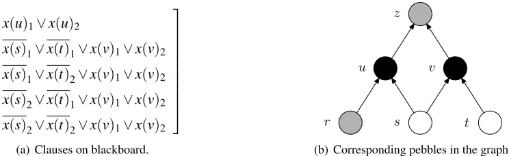
Using this intuitive correspondence, we can translate sets of clauses in a resolution refutation of

Pebd_Ginto black and white pebbles onGas inFigure 3. It is easy to see that if we assumex(s)1∨x(s)2

andx(t)1∨x(t)2, this assumption together with the clauses on the blackboard in Figure 3(a) imply

x(v)1∨x(v)2, sovshould be black-pebbled andsandtwhite-pebbled inFigure 3(b). The vertexuis also

black sincex(u)1∨x(u)2certainly is implied by the blackboard. This translation from clauses to pebbles

is quite straightforward, and seems to yield well-behaved pebblings for all “sensible” refutations ofPebd_G. The problem is that we have no guarantee that the resolution refutations will be “sensible.” Even though it might seem more or less clear how an optimal refutation of a pebbling contradiction should proceed, a particular refutation might contain unintuitive and seemingly non-optimal derivation steps that do not make much sense from a pebble game perspective. In particular, a resolution derivation has no obvious reason always to derive truth that is restricted to single vertices. For instance, it could add the axiomsx(u)_i∨x(v)₂∨x(z)1∨x(z)2,i=1,2, to the blackboard inFigure 3(a), derive that the

truth ofsandtimplies the truth of eithervorz, i. e., the clausesx(s)_i∨x(t)_j∨x(v)1∨x(z)1∨x(z)2for

i,j=1,2, and then erasex(u)1∨x(u)2from the blackboard. Although it is hard to see from such a small

(12)

         

x(u)1∨x(u)2

x(s)₁∨x(t)₁∨x(v)1∨x(v)2

x(s)₁∨x(t)₂∨x(v)1∨x(v)2

x(s)₂∨x(t)₁∨x(v)1∨x(v)2

x(s)₂∨x(t)₂∨x(v)1∨x(v)2

         

(a) Clauses on blackboard.

z

u v

r s t

(b) Corresponding pebbles in the graph.

Figure 3: Example of intuitive correspondence between sets of clauses and pebbles.

      

x(s)₁∨x(t)₁∨x(v)1∨x(z)1∨x(z)2

x(s)₁∨x(t)₂∨x(v)1∨x(z)1∨x(z)2

x(s)₂∨x(t)₁∨x(v)1∨x(z)1∨x(z)2

x(s)₂∨x(t)₂∨x(v)1∨x(z)1∨x(z)2

      

(a) New set of clauses on blackboard.

z

u v

r s t

(b) Corresponding blobs and pebbles.

Figure 4: Interpreting sets of clauses as black blobs and white pebbles.

such derivation steps in terms of black and white pebbles without making some component in the proof idea inSection 2.2break down.

Instead, what we do is to invent a new pebble game, with white pebbles just as before, but with black

blobsthat can cover multiple vertices instead of single-vertex black pebbles. A blob on a vertex setV can be thought of as truth of some vertexv∈V. The derivation sketched in the preceding paragraph, resulting in the set of clauses inFigure 4(a), will then be translated into white pebbles onsandtas before and a black blob covering bothvandzinFigure 4(b). We define rules in thisblob-pebble gamecorresponding roughly to black and white pebble placement and removal in the usual black-white pebble game, and add a specialinflation ruleallowing us to inflate black blobs to cover more vertices.

Once we have this blob-pebble game, we use it to construct a lower bound proof as outlined in

Section 2.2. First, we establish that for a fairly general class of graphs—namelylayeredgraphs, where the vertices can be divided into layers and all edges go between consecutive layers—any resolution refutation of a pebbling contradiction can be interpreted as a blob-pebbling on the DAG in terms of which this pebbling contradiction is defined. Intuitively, the reason that this works is that we can use the inflation rule to analyze apparently non-optimal steps in the refutation.

(13)

In fact, the only property that we need from the layered graphs inTheorem 2.1is that ifwis a vertex with (immediate) predecessorsuandv, then there is no path between the siblingsuandv. The theorem holds for any DAG satisfying this condition.

Next, we carefully design a cost function for black blobs and white pebbles so that the cost of the blob-pebblingPπ inTheorem 2.1is related to the space of the resolution refutationπ.

Theorem 2.2. Ifπis a refutation of a pebbling contradiction PebdGof degree d>1, then the cost of the

associated blob-pebblingP_π is bounded by the space ofπbycost(Pπ)≤Sp(π) +O(1).

Without going into too much detail, in order to make the proof ofTheorem 2.2work we can only charge for black blobs having distinct lowest vertices (measured in topological order), so additional blobs with the same bottom vertices are free. Also, we can only charge for white pebbles below these bottom vertices.

Finally, we need lower bounds on blob-pebbling price. Because of the inflation rule in combination with the peculiar cost function, the blob-pebble game seems to behave rather differently from the standard black-white pebble game, and therefore we cannot appeal directly to known lower bounds on black-white pebbling price. However, for a more restricted class of graphs than inTheorem 2.1, but still including binary trees and pyramids, we manage to prove tight bounds on the blob-pebbling price by generalizing the lower bound construction for black-white pebbling in [42].

Theorem 2.3. Any so-calledlayered spreading graphGhof height h has blob-pebbling priceΘ(h). In

particular, this holds for pyramid graphsΠh.

Putting all of this together, we can prove our main theorem.

Theorem 1.1(restated). Let Pebd_Π

h denote the pebbling contradiction of degree d>1over the pyramid graph of height h. Then the clause space of refuting Pebd_Πh by resolution is Sp(Pebd_Πh ` ⊥) =Θ(h).

Proof. The upper boundSp(Pebd_Πh ` ⊥) =O(h)is easy. A pyramid of height hcan be pebbled with

h+O(1)black pebbles, and a resolution refutation can mimic such a pebbling in constant extra clause space (independent ofd) to refute the corresponding pebbling contradiction.

The interesting part is the lower bound. Letπbe any resolution refutation ofPebd_Πh. Consider the associated blob-pebblingPπ provided byTheorem 2.1. On the one hand, we know that it holds that

cost(Pπ) =O(Sp(π))byTheorem 2.2, provided thatd>1. On the other hand,Theorem 2.3tells us that

the cost of any blob-pebbling ofΠhisΩ(h), so in particular we must havecost(Pπ) =Ω(h). Combining

these two bounds oncost(Pπ), we see thatSp(π) =Ω(h).

The pebbling contradictionPebd_Gis a (2+d)-CNF formula and for constantdthe size of the formula is linear in the number of verticesnofG(compareFigure 2). Thus, for pyramid graphsΠhthe corresponding pebbling contradictionsPebd_Πh have size quadratic in the heighth. Also, whendis fixed the upper bounds mentioned at the end ofSection 2.1becomeL(Pebd_G`⊥) =O(n)andW(Pebd_G`⊥) =O(1).Corollary 1.2

now follows if we setFn=PebdΠh ford=k−2 andh=b

√

ncand useTheorem 1.1.

Corollary 1.2(restated). For all k≥4, there is a family of k-CNF formulas{Fn}∞

n=1of sizeO(n)such

that L(Fn` ⊥) =O(n)and W(Fn` ⊥) =O(1)but Sp(Fn` ⊥) =Θ( √

(14)

2.4 Paper organization

Section 3provides formal definitions of the concepts introduced in Sections1and2. The bulk of the paper is then spent proving the lower-bound part of our main result inTheorem 1.1. InSection 4, we define our modified pebble game, the “blob-pebble game,” that we will use to analyze resolution refutations of pebbling contradictions. InSection 5we prove that resolution refutations can be translated into pebblings in this game, which isTheorem 2.1inSection 2.3. InSection 6, we proveTheorem 2.2 saying that the blob-pebbling price accurately measures the clause space of the corresponding resolution refutation. Finally, after giving a fairly detailed exposition of the lower bound on black-white pebbling of [42] in

Section 7(with a somewhat simplified analysis tailor-made for our purposes), inSection 8we delve into the details of the proof construction and modify it to apply to our blob-pebble game. This gives us

Theorem 2.3. NowTheorem 1.1andCorollary 1.2follow as in the proofs given at the end ofSection 2.3. We conclude inSection 9by giving suggestions for further research.

3 Formal preliminaries

In this section, we define resolution, pebble games and pebbling contradictions. This is standard material and much of the discussion below is identical or very close to similar sections in [15,47,49].

3.1 The resolution proof system

Aliteralis either a propositional logic variablexor its negation, denotedx. We definex=x. Two literals

aandbarestrictly distinctifa6=banda6=b, i. e., if they refer to distinct variables.

Aclause C=a1∨ · · · ∨ak is a set of literals. Throughout this paper, without loss of generality all clausesC are assumed to be nontrivial in the sense that all literals inCare pairwise strictly distinct (otherwiseCis trivially true since it contains some variable and its negation, and it is easy to show that such clauses can be ignored). We say thatCis asubclauseofDifC⊆D. A clause containing at mostk

literals is called ak-clause.

ACNF formula F=C₁∧ · · · ∧Cmis a set of clauses. Ak-CNF formulais a CNF formula consisting ofk-clauses. We define thesize S(F)of the formulaFto be the total number of literals inFcounted with repetitions. More often, we will be interested in the number of clauses|F|ofF.

In this paper, when nothing else is stated it is assumed thatA,B,C,Ddenote clauses;C,Dsets of

clauses;x,ypropositional variables;a,b,c literals;α,β truth value assignments; and ν a truth value

0 (false) or 1 (true). We write

αx=ν(y) = (

α(y) ify6=x, ν ify=x,

(3.1)

to denote the truth value assignment that agrees withα everywhere except possibly atx, to which it

assigns the valueν. We letVars(C)denote the set of variables andLit(C)the set of literals in a clauseC.3 This notation is extended to sets of clauses by taking unions. Also, we employ the standard notation [n] ={1,2, . . . ,n}.

(15)

A resolution derivationπ:F`Aof a clause A from a CNF formulaF is a sequence of clauses π={D1, . . . ,Dτ}such thatDτ =Aand each lineDi,i∈[τ], either is one of the clauses inF (anaxiom

clause) or is derived from clausesDj,Dkinπwith j,k<iby theresolution rule B∨x C∨x

B∨C . (3.2)

We refer to (3.2) asresolution on the variable xand toB∨Cas theresolventofB∨xandC∨xonx. A

resolution refutationof a CNF formulaFis a resolution derivation of the empty clause⊥(the clause with no literals) fromF. Perhaps somewhat confusingly, this is sometimes also referred to in the literature as a

resolution proof ofF, and we will use the two terms “proof” and “refutation” interchangeably in this paper.

For a formulaF and a set of formulasG={G1, . . . ,Gn}, we say thatGimplies F, denotedGF,

if every truth value assignment satisfying all formulasG∈GsatisfiesF as well. It is well known that resolution is sound and implicationally complete. That is, if there is a resolution derivationπ:F`A, then FA, and ifFA, then there is a resolution derivationπ:F`A0for someA0⊆A. In particular,Fis

unsatisfiable if and only if there is a resolution refutation ofF.

With every resolution derivationπ:F`Awe can associate a DAGGπ, with the clauses inπlabelling

the vertices and with edges from the assumption clauses to the resolvent for each application of the resolution rule (3.2). There might be several different derivations of a clauseCinπ, but if so we can

label each occurrence ofC with a timestamp when it was derived and keep track of which copy of

Cis used where. A resolution derivationπ istree-likeif any clause in the derivation is used at most once as a premise in an application of the resolution rule, i. e., ifGπis a tree. (We may make different

“time-stamped” vertex copies of the axiom clauses in order to makeG_πinto a tree.)

Thelength L(π)of a resolution derivationπis the number of clauses in it, counted with repetitions. We define the length of deriving a clauseAfrom a formulaFasL(F`A) =minπ:F`A{L(π)}, where the minimum is taken over all resolution derivations ofA. In particular, the length of refutingFby resolution is denotedL(F` ⊥).

Thewidth W(C)of a clauseCis|C|, i. e., the number of literals appearing in it. The width of a set of clausesCisW(C) =maxC∈C{W(C)}. The width of derivingAfromF by resolution isW(F`A) =

minπ:F`A{W(π)}, and the width of refutingFis denotedW(F` ⊥).

We next define the measure ofspace. Following the exposition in [31], a proof can be seen as a Turing machine computation, with a special read-only input tape from which the axioms can be downloaded and a working memory where all derivation steps are made. Theclause spaceof a resolution proof is the maximum number of clauses that need to be kept in memory simultaneously during a verification of the proof. Thetotal space4is the maximum total space needed, where also the width of the clauses is taken into account. For the formal definitions, it is convenient to use an alternative definition of resolution introduced in [2].

Definition 3.1(Resolution). Aclause configurationCis a set of clauses. A sequence of clause

configu-rations{_C₀, . . . ,Cτ}is aresolution derivationfrom a CNF formulaF ifC0=/0 and for allt∈[τ],Ct is obtained fromCt−1by one of the following rules:

(16)

Axiom download Ct =Ct−1∪ {C}for someC∈F.

Erasure Ct=Ct−1\ {C}for someC∈Ct−1.

Inference Ct =Ct−1∪ {D}for someDinferred by resolution fromC1,C2∈Ct−1.

A resolution derivationπ:F`Aof a clauseAfrom a formulaF is a derivation{C0, . . . ,Cτ}such that Cτ ={A}. Aresolution refutationofF is a derivation of the empty clause⊥fromF.

Definition 3.2(Clause space [2,12]). Theclause spaceof a resolution derivationπ ={C0, . . . ,Cτ}

is maxt∈[τ]{|Ct|}. The clause space of deriving the clause A from the formula F is Sp(F`A) = minπ:F`A{Sp(π)}, andSp(F` ⊥)denotes the minimum clause space of any resolution refutation ofF. Definition 3.3(Total space [2]). Thetotal spaceof a clause configurationCisTotSp(C) =∑C∈CW(C).

The total space of a resolution derivation{_C₀, . . . ,Cτ}is maxt∈[τ]{TotSp(Ct)}, andTotSp(F` ⊥)is the minimum total space of any resolution refutation ofF.

In this paper, we will be almost exclusively interested in the clause space of general, unrestricted resolution refutations. When we write simply “space” for brevity, we mean clause space in general resolution.

3.2 Pebble games and pebbling contradictions

Pebble games were originally devised for studying programming languages and compiler construction, but have later found a variety of applications in computational complexity theory. In connection with resolution, pebble games have been used both to analyze resolution derivations with respect to how much memory they consume (using the original definition of space in [31]) and to construct CNF formulas which are hard for different variants of resolution in various respects (see for example [3,14,19,21]). An excellent survey of pebbling up to ca. 1980 is [51]. A second article, with more narrow focus but covering some more recent developments, is the first author’s upcoming survey [48].

Theblack pebbling priceof a DAGGcaptures the amount of memory, i. e., the number of registers, required to perform the deterministic computation described byG. The space of a non-deterministic computation is measured by theblack-white pebbling priceofG. We say that vertices ofGwith indegree 0 aresourcesand that vertices with outdegree 0 aresinksortargets. In the following, unless otherwise stated we will assume that all DAGs under discussion have a unique sink, and this sink will always be denotedz. The next definition is adapted from [27], though we use the established pebbling terminology introduced by [39].

Definition 3.4(Pebble game). Suppose thatGis a DAG with sourcesSand a unique sinkz. The black-white pebble gameonGis the following one-player game. At any point in the game, there are black and white pebbles placed on some vertices ofG, at most one pebble per vertex. Apebble configuration

is a pair of subsetsP= (B,W)ofV(G), comprising the black-pebbled verticesBand white-pebbled

verticesW. The rules of the game are as follows:

(17)

2. A black pebble may be removed from any vertex at any time.

3. A white pebble may be placed on any empty vertex at any time.

4. If all immediate predecessors of a white-pebbled vertexvhave pebbles on them, the white pebble onvmay be removed. In particular, a white pebble can always be removed from a source vertex.

A black-white pebbling from (B₁,W₁) to (B₂,W₂) in G is a sequence of pebble configurations P={_P₀, . . . ,Pτ}such thatP0= (B1,W1),Pτ = (B2,W2), and for allt∈[τ], Pt follows from Pt−1by

one of the rules above. If(B1,W1) = (/0,/0), we say that the pebbling isunconditional, otherwise it is

conditional.

Thecostof a pebble configurationP= (B,W)iscost(P) =|B∪W|and the cost of a pebblingP=

{P0, . . . ,Pτ}is max0≤t≤τ{cost(Pt)}. Theblack-white pebbling priceof(B,W), denotedBW-Peb(B,W), is the minimum cost of any unconditional pebbling reaching(B,W).

Acomplete pebblingofG, also called apebbling strategyforG, is an unconditional pebbling reaching ({z},/0). Theblack-white pebbling priceofG, denotedBW-Peb(G), is the minimum cost of any complete black-white pebbling ofG.

Ablack pebblingis a pebbling using black pebbles only, i. e., havingWt= /0 for allt. The(black)

pebbling priceofG, denotedPeb(G), is the minimum cost of any complete black pebbling ofG. We think of the moves in a pebbling as occurring at integral time intervalst=1,2, . . .and talk about the pebbling move “at timet” (which is the move resulting in configurationPt) or the moves “during the time interval[t1,t2].”

The only pebblings we are really interested in are complete pebblings ofG. However, when we prove lower bounds for pebbling price it will sometimes be convenient to be able to reason in terms of partial pebbling move sequences, i. e., conditional pebblings.

Apebbling contradictiondefined on a DAGGencodes the pebble game onGby postulating the sources to be true and the sink to be false, and specifying that truth propagates through the graph according to the pebbling rules. The definition below is a generalization of formulas previously studied in [19,53].

Definition 3.5(Pebbling contradiction [17]). Suppose thatGis a DAG with sourcesS, a unique sinkz

and with all non-source vertices having indegree 2, and letd>0 be an integer. Associated distinct variablesx(v)1, . . . ,x(v)d with every vertexv∈V(G). Thedth degreepebbling contradictionoverG, denotedPebd_G, is the conjunction of the following clauses:

• Wd

i=1x(s)ifor alls∈S(source axioms), • x(u)_i∨x(v)_j∨Wd

l=1x(w)l for alli,j∈[d]and allw∈V(G)\S, whereu,vare the two predecessors ofw(pebbling axioms).

• x(z)_ifor alli∈[d](sink axiomsortarget axioms),

The formula Pebd_Gis a (2+d)-CNF formula with O d2· |V(G)|

(18)

v

G_M\v GO

\

v

G\ G_Mv∪GO v

Figure 5: Notation for sets of vertices in DAGGwith respect to a vertexv.

4 A game for analyzing pebbling contradictions

We now start working on the proof ofTheorem 1.1, which will require the rest of this paper. In this section we present the modified pebble game that we will use to study the clause space of resolution refutations of pebbling contradictions. We remark that the game has been somewhat simplified as compared to the preliminary version [50] of this paper, incorporating some ideas from [15].

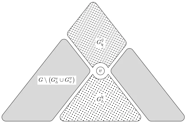
4.1 Some graph notation and definitions

We first present some notation and terminology that will be used in what follows. SeeFigure 5for an illustration of the next definition.

Definition 4.1(Graph notation). We letsucc(v)denote the immediate successors andpred(v)denote the immediate predecessors of a vertexvin a DAGG. We will usually drop the prefix “immediate” so that the terms “successor” and “predecessor” refer to an immediate successor or predecessor, respectively, unless stated otherwise.

Taking the transitive closures ofsucc(·)andpred(·), we letGO_v denote all vertices reachable fromv

(vertices “above”v) andG_Mv denote all vertices from whichvis reachable (vertices “below”v). We write

G_M\v andGO_\_v to denote the corresponding sets with the vertexvitself removed.

Ifpred(v) ={u,w}, we say thatuandwaresiblings. Ifu6∈G_Mv andv6∈G_Mu, we say thatuandvare

non-comparablevertices. Otherwise they arecomparable.

(19)

When reasoning about arbitrary vertices we will often use as a canonical example a vertexrwith assumed predecessorspred(r) ={p,q}.

Note that for a leafvwe havepred(v) =/0, and for the sinkzofGwe havesucc(z) = /0. Also note thatG_Mv andGO_v are sets of vertices, not subgraphs. However, we will allow ourselves to overload the notation and frequently use it for both the subgraph and its vertex set. In a similar fashion, as a rule we will overload the notation for the graphGitself and its vertices, and usually write onlyGwhen we meanV(G), and when this should be clear from context.

In this paper, we will focus onlayereddirected acyclic graphs. Let us give a formal definition of this concept for completeness.

Definition 4.2(Layered DAG). Alayered DAGis a DAG whose vertices are partitioned into (nonempty) sets oflayers V0,V1, . . . ,Vhonlevels0,1, . . . ,h, and whose edges run between consecutive layers. That is, if(u,v)is a directed edge, then the level ofuisL−1 and the level ofvisLfor someL∈[h]. We say that

his theheightof the layered DAG.

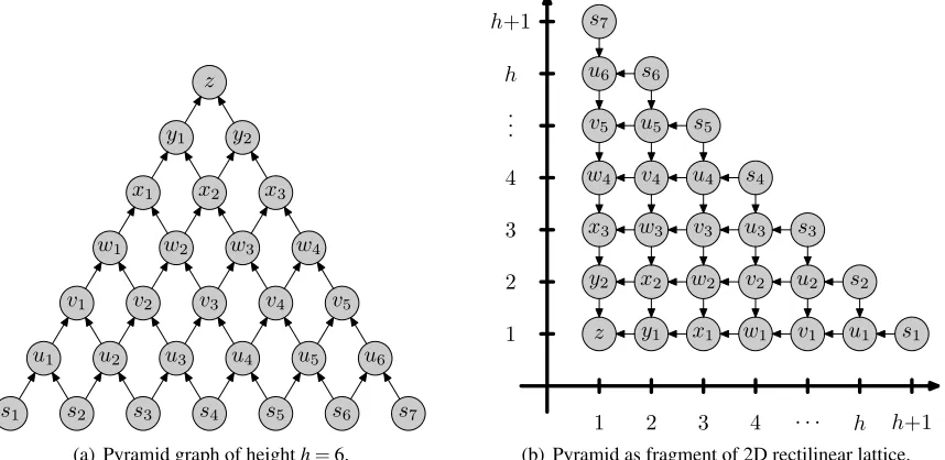
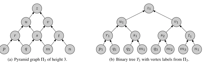
Throughout this paper, we will assume that all source vertices in a layered DAG are located on the bottom level 0. A family of layered DAGs that will be of particular interest to us are so-calledpyramid graphs, which are defined as follows.

Definition 4.3(Pyramid graph). Thepyramid graphΠhof heighthis a layered DAG withh+1 levels, where there is one vertex on the highest level (the sinkz), two vertices on the next level et cetera down to

h+1 vertices at the lowest level 0. Theith vertex at levelLhas incoming edges from theith and(i+1)st vertices at levelL−1.

We also need some notation for contiguous and non-contiguous topologically ordered sets of vertices in a DAG.

Definition 4.4(Paths and chains). We say thatV is a(totally) orderedset of vertices in a DAGG, or a

chain, if all vertices inV are comparable (i. e., if for allu,v∈V, eitheru∈G_Mv orv∈G_Mu). Apath Pis a contiguous chain, i. e., such thatsucc(v)∩P6= /0 for allv∈Pexcept the top vertex.

We writeP:v wto denote a path starting invand ending inw. Asource pathis a path that starts at some source vertex ofG. Apath via wis a path such thatw∈P. We will also say thatP visits w.

For a chainV we writeP_via(V)denote the set of all source paths that visit all vertices inV, or that

agreewithV. Also, we writeS

Pvia(V)for the union of all vertices in pathsP∈Pvia(V).

4.2 Description of the blob-pebble game and formal definition

To prove a lower bound on the refutation space of pebbling contradictions, we want to interpret derivation steps in terms of pebble placements and removals in the corresponding graph. InSection 2, we outlined an intuitive correspondence between clauses and pebbles. The problem is that if we try to use this correspondence, the pebble configurations that we get do not obey the rules of the black-white pebble game. Therefore, we are forced to to change the pebbling rules. In this section, we present the modified pebble game used for analyzing resolution derivations.

(20)

make the correspondence between pebblings and resolution derivations much more natural. Clearly, this is only a minor adjustment, and it is easy to prove formally that it does not really change anything.

Our second, and far more substantial, modification of the pebble game is motivated by the fact that in general, a resolution refutation a priori has no reason to follow our pebble game intuition. Since pebbles are induced by clauses, if at some derivation step the refutation chooses to erase “the wrong clause” from the point of view of the induced pebble configuration, this can lead to pebbles just disappearing. Whatever our translation from clauses to pebbles is, a resolution proof that suddenly out of spite erases practically all clauses must surely lead to practically all pebbles disappearing, if we want to maintain a correspondence between clause space and pebbling cost. This is all in order for black pebbles, but if we allow uncontrolled removal of white pebbles we cannot hope for any nontrivial lower bounds on pebbling price (to see this, just white-pebble the two predecessors of the sink, then black-pebble the sink itself and finally remove the white pebbles).

Our solution to this problem is to keep track of exactly which white pebbles have been used to get a black pebble on a vertex. Loosely put, removing a white pebble from a vertexvwithout placing a black pebble on the same vertex should be in order, provided that all black pebbles placed on vertices abovevin the DAG with the help of the white pebble onvare removed as well. We do the necessary bookkeeping by definingsubconfigurationsof pebbles, each subconfiguration consisting of a black pebble together with all the white pebbles this black pebble depends on, and requiring that if any pebble in a subconfiguration is removed, then all other pebbles in this subconfiguration must be removed as well.

Another problem is that resolution derivation steps can be made that appear intuitively bad given that we know that the end goal is to derive the empty clause, but where formally it appears hard to nail down wherein this supposed badness lies. To analyze such apparently non-optimal derivation steps, we introduce aninflationrule in which a black pebble can be inflated to ablobcovering multiple vertices. The way to think of this is that a black pebble on a vertexvcorresponds to derived truth ofv, whereas for a blob pebble onV we only know that some vertexv∈V is true, but not which one.

We now present the formal definition of the concept used to “label” each black blob pebble with the set of white pebbles (if any) this black pebble is dependent on. The intended meaning of the notation [B]hWiis a black blob onBtogether with the white pebblesW belowBwith the help of which we have been able to place the black blob onB. We refer to the structure[B]hWigrouping together a black blobB

and its associated white pebblesW as ablob subconfiguration, or justsubconfigurationfor short.

Definition 4.5(Blob subconfiguration). For sets of verticesB,W in a DAGG,[B]hWiis ablob subcon-figurationifB6= /0 andB∩W = /0. We refer toBas a (single) blackbloband toW as (a number of different) white pebblessupporting B. We also say thatBisdependentonW. IfW=/0,Bisindependent. BlobsBwith|B|=1 are said to beatomic. A set of blob subconfigurationsS=[Bi]hWii |i=1, . . . ,m together constitute ablob-pebbling configuration.

Since the definition of the game we will play with these blobs and pebbles is somewhat involved, let us first try to give an intuitive description.

(21)

• The analogy forrule 2for black pebble removal inDefinition 3.4is a rule for “shrinking” black blobs. A vertexvin a blob can be eliminated bymergingtwo blob subconfigurations, provided that there is both a black blob and a white pebble onv, and provided that the two black blobs involved in thismerger do not intersect the supporting white pebbles of one another in any other vertex thanv. Removing black pebbles in the black-white pebble game corresponds to shrinking atomic black blobs.

• A black blob can beinflatedto cover more vertices, as long as it does not collide with its own supporting white vertices. Also, new supporting white pebbles can be added at an inflation move. There is no analogy of this move in the usual black-white pebble game.

• Therule 4for white pebble removal also corresponds to merging in the blob-pebble game, in the sense that the white pebble used in the merger is eliminated as well.

• Other than that, individual white pebbles, and individual black vertices covered by blobs, can never just disappear. If we want to remove a white pebble or parts of a black blob, we can do so only by

erasingthe whole blob subconfiguration.

The formal definition follows. SeeFigure 6for some examples of blob-pebbling moves.

Definition 4.6(Blob-pebble game). LetGbe a DAG with unique sinkz. Theblob-pebbling rulesfor going from a blob-pebbling configurationS0 to a blob-pebbling configurationSonGare as follows:

Introduction S=S0∪[v]hpred(v)i for anyv∈V(G).

Merger S=S0∪[B]hWi if there are[B1]hW1i,[B2]hW2i ∈S0 such that

1. B1∩W2=/0,

2. |B2∩W1|=1; letv∗denote this unique element inB2∩W1,

3. B=B1∪(B2\ {v∗}) = (B1∪B2)\ {v∗}, and

4. W= (W1\ {v∗})∪W2= (W1∪W2)\ {v∗}.

We write[B]hWi=merge([B₁]hW₁i,[B₂]hW₂i)and refer to this as amerger on v∗.

Inflation S=S0∪[B]hWi if there is a[B0]hW0i ∈S0such thatB⊇B0andW⊇W0.

We say that the blob-pebbling configuration[B]hWiis derived from[B0]hW0ibyinflationor that [B0]hW0iisinflatedto yield[B]hWi.

Erasure S=S0\[B]hWi for[B]hWi ∈S0.

Ablob-pebbling moveat timet fromSt−1 toSt is either an introduction or any sequence of mergers, inflations and erasures.

For blob-pebbling configurationsS0andSτ onG, ablob-pebblingfromS0toSτ inGis a sequence

P=S0, . . . ,Sτ of blob-pebbling moves. The blob-pebblingPisunconditionalifS0=/0 andconditional

otherwise. Acomplete blob-pebblingofGis an unconditional pebblingPending inSτ =

[z]h/0i forz

(22)

(a) Empty pyramid. (b) Introduction move.

(c) Two subconfigurations before merger. (d) The merged subconfiguration.

(e) Subconfiguration before inflation. (f) Subconfiguration after inflation.

(23)

4.3 Blob-Pebbling price

We have not yet defined what the price of a blob-pebbling is. The reason is that it is not a priori clear what the “correct” definition of blob-pebbling price should be.

It should be pointed out that the blob-pebble game has no obvious intrinsic value—its function is to serve as a tool to prove lower bounds on the resolution refutation space of pebbling contradictions. The intended structure of our lower bound proof for resolution space is that we want look at resolution refutations of pebbling contradictions, interpret them in terms of blob-pebblings on the underlying graphs, and then translate lower bounds on the price of these blob-pebblings into lower bounds on the size of the corresponding clause configurations. Therefore, we have two requirements for the blob-pebbling price Blob-Peb(G):

1. It should be sufficiently high, i. e., sufficiently similar to standard black-white pebbling price to enable us to prove good lower bounds onBlob-Peb(G), preferrably by making it possible to use lower bound proof techniques forBW-Peb(G)to obtain analogous bounds forBlob-Peb(G). 2. It should also be sufficiently low, in the sense that it should take into consideration the way

subconfigurations are obtained from clauses in resolution derivations, so that lower bounds on Blob-Peb(G)translate back to lower bounds on the size of the clause configurations.

Hence, when defining pebbling price inDefinition 4.7below, we should also have to have in mind the comingDefinition 5.2saying how we will interpret clauses in terms of blobs and pebbles, so that these two definitions together make it possible for us to get a lower bound on clause set size in terms of pebbling cost.

For black pebbles, we could try to charge 1 for each distinct blob. But this will not work, since then the second requirement above fails. For the translation of clauses to blobs and pebbles sketched in

Section 2.3it is possible to construct clause configurations that correspond to an exponential number of distinct black blobs measured in the clause set size. The other natural extreme seems to be to charge only for mutually disjoint black blobs. But this is far too generous, and the first requirement above fails. To get a trivial example of this, take any ordinary black pebbling ofGand translate in into an (atomic) blob-pebbling, but then change it so that each black pebble[v]is immediately inflated to[{v,z}]after each introduction move. It is straightforward to verify that this would yield a pebbling ofGin constant cost. For white pebbles, the first idea might be to charge 1 for every white-pebbled vertex, just as in the standard pebble game. On closer inspection, though, this turns out to lead to technical problems in the proofs, and so this seems to be not quite what we need.

The definition presented below turns out to give us both of the desired properties above, and allows us to prove an optimal bound. Namely, we define blob-pebbling price so as to charge 1 foreach distinct bottom vertexthat is the unique bottom vertex of its black blob, and so as to charge for the subset of supporting white pebblesW ∩Gb_Min a subconfiguration[B]hWithat arelocated below all bottom vertices

bot(B)of its black blobB. Multiple distinct blobs with the same bottom vertex come for free, however, as do blobs that do not have a unique bottom vertex. Also, any supporting white pebbles that are not “completely below” its own blob in the sense described above are also free, although we still have to keep

(24)

Definition 4.7 (Blob-pebbling price). For a blob subconfiguration [B]hWi, we define B([B]hWi) = {bot(B)} to be a chargeable black vertex if |bot(B)|=1 and setB([B]hWi) = /0 otherwise. We say thatWM([B]hWi) =W ∩T

b∈bot(B)GMb are the chargeable white vertices. The chargeable vertices of

the subconfiguration[B]hWiare all vertices in the unionB([B]hWi)∪WM_([_B_]_h_W_i₎_{. This definition is}

extended to blob-pebbling configurationsSin the natural way by lettingB(S) =S[B]hWi∈_SB([B]hWi)

andWM(S) =S[B]hWi∈SWM([B]hWi).

The cost of a blob-pebbling configurationSiscost(S) =B(S)∪WM(S)

, and the cost of a blob-pebblingP=S0, . . . ,Sτ iscost(P) =maxt∈[τ]

cost(St) .

Theblob-pebbling priceof a blob subconfiguration[B]hWi, denotedBlob-Peb([B]hWi), is the minimal cost of any unconditional blob-pebblingP={_S₀, . . . ,Sτ}such thatSτ=

[B]hWi . The blob-pebbling price of a DAGG isBlob-Peb(G) =Blob-Peb([z]h/0i), i. e., the minimal cost of any complete blob-pebbling ofG.

We will also writeW(S)to denote the set of all white-pebbled vertices inS, including non-chargeable

ones.

We stress again that we make no claim thatDefinition 4.7is the “obviously correct” definition of blob-pebbling price—it just happens to be a definition that works. In fact, there are other possible options, some of which are arguably more natural but lead to more complicated proofs or slightly worse bounds. To conclude this section, we just want to mention one alternative definition which seems slightly more natural to us, which yields a slightly stronger pebbling price, and which might therefore be useful if lower bounds on blob-pebbling price are to be extended from layered graphs to more general DAGs (as discussed inSection 9).

Namely, forB1, . . . ,Bmany sets of vertices, let us say that aset of distinguished representativesfor

B₁, . . . ,Bmis a setR={b1, . . . ,bm}wherebi∈Bi\

S

j<iBj for all i∈[m]. Note that in general, such sets of distinguished representatives need not exist, but we can always find apartial set of distinguished representativesfor B1, . . . ,Bm, which we define to be a set of distinguished representatives for some

(ordered) subsetBi1, . . . ,Bisof the vertex sets. Now we can define the cost of a blob-pebbling configuration Sto be

cost(S) =max

R

R∪WM(S)

(4.1)

where the maximum is taken over all partial sets of distinguished representativesRfor the black blobs in

S.

The proof ofTheorem 6.5, which says that the clause space of a resolution refutation is lower bounded by the cost of the pebbling it induces, can be adapted to work for this definition if one proves first a lower bound for black blobs only and then a second lower bound for white pebbles only, and finally combine them in the obvious way by taking the maximum of the two bounds. Unfortunately, this loses a constant factor of 2, and for reasons explained inSection 9we are interested in getting exactly the right multiplicative constants in this part of our argument. Therefore, in this paper we decided to stick with

(25)

5 Resolution derivations induce blob-pebblings

In this section, we show how resolution refutations of pebbling contradictions can be translated to blob-pebblings (as described inDefinition 4.6) of the corresponding DAGs. For simplicity, in the current section, as well as in the next one, we will writev1,v2, . . . ,vd instead ofx(v)1,x(v)2, . . . ,x(v)d for thed variables associated withvin adth degree pebbling contradiction. That is, in Sections5and6small letters with subscripts will denote variables in propositional logic only and nothing else.

It turns out that for technical reasons, it is convenient to ignore the target axioms z1, . . . ,zd in a pebbling contradiction and focus on resolution derivations ofWd

l=1zl from the rest of the formula rather than resolution refutations of all ofPebd_G. Let us write *Pebd_G=Pebd_G\

z1, . . . ,zd to denote the pebbling formula overGwith the target axioms in the pebbling contradiction removed. The next lemma is the formal statement saying that we may just as well study derivations ofWd

l=1zl from *PebdGinstead of refutations ofPebd_G.

Lemma 5.1. For any DAG G with sink z, it holds that Sp(Pebd_G` ⊥) =Sp(*Pebd_G`Wd

l=1zl).

Proof. From any resolution derivationπ∗: *Pebd_G`Wd_l=₁zl, we can obtain a resolution refutation ofPebdG fromπ∗in the same space by resolving the final clauseWd

l=1zl with all sink axiomszl,l=1, . . . ,d, one by one in space 3.

In the other direction, forπ:Pebd_G` ⊥we can extract a derivation ofWd_l=₁zl in at most the same space by simply omitting all downloads of and resolution steps onzlinπ, leaving the literalszl in the clauses. Instead of the final empty clause⊥we get some clauseD⊆Wd

l=1zl, and since *PebdG2D$

Wd

l=1zl and resolution is sound, we haveD=Wd

l=1zl.

In view ofLemma 5.1, from now on we will only consider resolution derivations from *Pebd_Gand try to convert clause configurations in such derivations into sets of blob subconfigurations.

To avoid cluttering the notation with an excessive amount of brackets, we will sometimes use sloppy notation for sets. We will allow ourselves to omit curly brackets around singleton sets when this is clear from context, writing e. g.,V ∪vinstead ofV ∪ {v}and[B∪b]hW∪wiinstead of[B∪ {b}]hW ∪ {w}i. Also, we will sometimes omit the curly brackets around sets of vertices in black blobs and write, e. g., [u,v]instead of[{u,v}].

5.1 Definition of induced configurations and theorem statement

Ifris a non-source vertex withpred(r) ={p,q}, we say that theaxioms for rin *Pebd_Gis the set

Axd(r) =p_i∨q_j∨Wd

l=1rl|i,j∈[d] (5.1) and if r is a source, we define Axd(r) =Wd

i=1ri . ForV a set of vertices in G, we letAxd(V) =

Axd(v)|v∈V . Note that with this notation, we have *Pebd_G=Axd(v)|v∈V(G) . For brevity, we introduce the shorthand notation

And+(V) =Wd

i=1vi|v∈V , (5.2a)

Or+(V) =W

v∈V

Wd

(26)

The reader can think ofAnd+(V)as “truth of all vertices inV” andOr+(V)as “truth of some vertex inV.” We say that a set of clausesCimplies a clauseD minimallyifCDbut for allC0$ Cit holds that C02D. IfC⊥minimally,Cis said to beminimally unsatisfiable. We say thatCimplies a clauseD maximallyifCDbut for allD0$Dit holds thatC 2D0. To define our translation of clauses to blob

subconfigurations, we use implications that are in a sense both minimal and maximal.

Definition 5.2(Induced blob subconfiguration). LetGbe a DAG andCa clause configuration derived

from *Pebd_G. ThenCinduces the blob subconfiguration[B]hWiif there is a clause setD⊆Csuch that

D∪And+(W)Or+(B) (5.3a)

but for which it holds for all strict subsetsD0$ D,W0$W andB0$Bthat

D0∪And+(W)2Or+(B), (5.3b) D∪And+(W0)2Or+(B),and (5.3c) D∪And+(W)2Or+(B0). (5.3d)

We writeS(C)to denote the set of all blob subconfigurations induced byC. To save space, when all

conditions (5.3a)–(5.3d) hold, we write

D∪And+(W)BOr+(B) (5.4)

and refer to this asprecise implicationor say that the clause setD∪And+(W)implies the clauseOr+(B) precisely. Also, we say that the precise implicationD∪And+(W)BOr+(B)witnessesthe induced blob

subconfiguration[B]hWi.

Let us see that this definition agrees with the intuition presented inSection 2.3. An atomic black pebble on a single vertexvcorresponds, as promised, to the fact thatWd

i=1viis implied by the current set of clauses. A black blob onV without supporting white pebbles is induced precisely when the disjunctionOr+(V) =W

v∈V

Wd

i=1viof the corresponding clauses follow from the clauses in memory, but no disjunction over a strict subset of verticesV0$V is implied. Finally, the supporting white pebbles just

indicate that if we indeed had the information corresponding to black pebbles on these vertices, the clause corresponding to the supported black blob could be derived. Remember that our cost measure does not take into account the size of blobs. This is natural since we are interested in clause space, and since large blobs, in an intuitive sense, corresponds to large (i. e., wide) clauses rather than many clauses.

We are now ready to state the main result of this section, which says that if we apply the translation of clauses to blobs and pebbles inDefinition 5.2on all the clause configurations in a resolution derivation ofWd

l=1zlfrom *PebdG, then we obtain essentially a legal blob-pebbling ofG. Theorem 5.3. Let π =C0, . . . ,Cτ be a resolution derivation of

Wd

i=1zi from*PebdG for a DAG G.

Then the induced blob-pebbling configurationsS(C0), . . . ,S(Cτ) form the “backbone” of a complete blob-pebblingPof G in the sense that:

• S(C0) = /0,

(27)

• for every t∈[τ], the transitionS(Ct−1) S(Ct) can be accomplished in accordance with the

blob-pebbling rules in costmax

cost(S(Ct−1)),cost(S(Ct)) +O(1).

In particular, to any derivationπ: *PebdG`

Wd

i=1ziwe can associate a complete blob-pebblingPπ of G such thatcost(Pπ)≤maxC∈π

cost(S(C)) +O(1).

We prove the theorem by forward induction over the derivationπ. By the pebbling rules in Def-inition 4.6, any subconfiguration [B]hWi may be erased freely at any time. Consequently, we need not worry about subconfigurations disappearing during the transition fromCt−1 toCt. What we do need to check, though, is that no subconfiguration[B]hWiappears inexplicably inS(Ct)as a result of a derivation stepCt−1 Ct, but that we can always derive any[B]hWi ∈S(Ct)\S(Ct−1)fromS(Ct−1)by

the blob-pebbling rules. Also, when several pebbling moves are needed to get fromS(Ct)toS(Ct−1),

we need to check that these intermediate moves do not affect the pebbling cost by more than an additive constant.

The proof boils down to a case analysis of the different possibilities for the derivation step to get fromCt−1toCt. Since the analysis is quite lengthy, we divide it into subsections. But first of all we need some auxiliary technical lemmas.

5.2 Some technical lemmas

The next three lemmas are not hard, but will prove quite useful. We present the proofs for completeness.

Lemma 5.4. LetCbe a set of clauses and D a clause such thatCD minimally and a∈Lit(C)but a6∈Lit(C). Then a∈Lit(D).

Proof. Suppose not. LetC1={C∈C|a∈Lit(C)}andC2=C\C1. SinceC22Dthere is a truth value

assignmentαsuch thatα(C2) =1 andα(D) =0. Note thatα(a) =0, since otherwiseα(C1) =1 which

would contradictC1∪C2=CD. It follows thata∈/Lit(D). Flipato true and denote the resulting

truth value assignment byαa=1. By constructionαa=1(C1) =1 andC2 andDare not affected since

{a,a} ∩ Lit(C2)∪Lit(D)

=/0, soαa=1(C) =1 andαa=1(D) =0. Contradiction.

Lemma 5.5. Suppose that C,D are clauses andCis a set of clauses. ThenC∪C D if and only if Ca∨D for all a∈Lit(C).

Proof. Assume thatC∪C Dand consider any assignmentα such thatα(C) =1 andα(D) =0 (if

there is no suchα, thenCD⊆a∨D). Such anα must setCto false, i. e., allato true. Conversely,

ifCa∨Dfor alla∈Lit(C)andα is such thatα(C) =α(C) =1, it must hold thatα(D) =1, since otherwiseα(a∨D) =0 for some literala∈Lit(C)satisfied byα.

Lemma 5.6. Suppose thatCD minimally. Then no literal from D can occur negated inC, i. e., it holds that{a|a∈Lit(D)} ∩Lit(C) =/0.

Proof. Suppose not. LetC1={C∈C| ∃asuch thata∈Lit(C)anda∈Lit(D)} and letC2=C\C1.

SinceC22Dthere is anα such thatα(C2) =1 andα(D) =0. But thenα(C1) =1, since everyC∈C1

Towards an Optimal Separation of Space and Length in Resolution