ALGEBRAIC DIFFERENCE EQUATIONS FOR STAND HEIGHT,
DIAMETER, AND VOLUME DEPENDING ON STAND AGE AND
SITE FACTORS FOR ESTONIAN STATE FORESTS
Andres Kiviste
1, K¨
ulliki Kiviste
21Professor,2Lecturer, IFRE, Estonian University of Life Sciences, Tartu, Estonia. Ph./FAX:(372)731-3156/3156
Abstract.Algebraic difference equations of stand height, diameter, and volume depending on dominant species and site factors have been explored on the basis of Estonian state forest inventory data. Stand variables such as total age, average height, breast height diameter, volume, origin (naturally regenerated or cultivated), forest site type and dominant species from forest inventory database files of Estonian state forests have been used as initial data for this study. A total of 171 data series of height, diameter and volume on age were calculated as averages of data groups by site type, dominant species, origin, and age classes of 5 years. The Cieszewski and Bella (1989) algebraic difference equation has been used for model construction. First, tree parameters of the Hossfeld function were estimated for each of the height, diameter and volume series and relationships between the parameters were later studied. In the final model, dominant tree species, thickness of organic layer of soil, stand origin, height, diameter, and volume at given age were used as input variables. The model is included in the Estonian state forest information system and in several software packages for forest inventory data processing.
Keywords:growth modeling, algebraic difference equation, height, diameter, volume
1
Introduction
The republic of Estonia lies in Eastern Europe be-tween latitudes 57o30’ and 59o49’ N and longitudes 21o46’ and 28o13’ E. The total area of forestland is 2.27 million ha, i.e. 51.9% of the area of Estonia. The vol-ume of growing stock on forestland is 451 million cubic meters and is showing a trend to increase. Pine stands have the largest area and growing stock (710 thousand ha and 151 million m3) while birch stands take second place (707 thousand ha and 118 million m3) and spruce stands take third place (404 thousand ha and 87 million m3) (Yearbook Forest 2004, 2005).
Phytogeographically, Estonia belongs to the northern part of the sub-belt of the nemoral coniferous or so-called mixed forests of the Northern Hemisphere’s temperate zone forest belt (Etverk et al 1995). The soils are very diverse due to big differences in parent material and in relief, as well as in the length of soil genesis and to a lesser extent in climatic conditions.
As a consequence of all this, forests of Estonia vary on a very large scale: there are dark boreal spruce forests with treetops at a height of 40 meters; heath pine forests, stunted in growth but full of sunshine; unique alvar
forests growing on a layer of soil that is only a few cen-timeters thick and lies on a stratum of limestone rock; and wet bog forests on peat layers several meters thick. An ordinated forest typological classification (L˜ohmus 1984) has been worked out. The set of Estonian forest site types is presented in Table 1. According to the dominant tree species there can be either one or several forest types in each site type.
Until recent times the forest growth and yield tables of Estonia and its nearest neighbors have been used in tonia to offer predictions of forest growth. However, Es-tonian forests are quite variable and the several growth tables of differing quality could not describe this variabil-ity well enough. Thus there has been a growing need for more general forest growth models.
From the aspect of modeling of Estonian forest growth, stand descriptions of state forest inventory are the most reliable data available in the state forest databases. Traditionally, state forest inventories take place every 10 years. During the forest inventory, ocular estimates of most stand variables (species composition, site type, stand age, height, diameter, volume, etc.) are assessed for each sub-compartment.
The purpose of the present study is to explore a model
Copyright c2009 Publisher of the International Journal ofMathematical and Computational Forestry & Natural-Resource Sciences
Table 1: Estonian forest site types by E. L˜ohmus (1984) and thickness of organic layer of soil (OHOR).
Code OHOR
cm
Site type Code OHOR
cm
Site type
LL 2 Arctostaphylos-alvar SL 1 Hepatica
KL 1 Calamagrostis-alvar ND 1 Aegopodium
SM 4 Cladonia SJ 15 Dryopteris
KN 5 Calluna AN 10 Filipendula
SN 20 Vaccinium uliginosum TAN 15 Carex-Filipendula
PH 4 Rhodococcum OS 20 Equisetum
JPH 4 Oxalis-Rhodococcum TR 20 Carex
MS 10 Myrtillus RB 50 Raised (oligotrophic) bog
JMS 6 Oxalis-Myrtillus SS 50 Transitional (mesotrophic) bog
KMS 13 Polytrichum-Myrtillus MDS 50 Alder-birch (eutrophic-mesotropic) swamp
KR 20 Polytrichum LD 50 Alder (eutrophic) fen
JK 4 Oxalis KS 50 Drained swamp
for prediction of the growth of stand height, diameter and volume using the present state of the stand and site variables.
2
Materials
As initial data for modeling, stand records of Estonian state forest inventory in 1984-1993 were used (Kiviste 1995, Kiviste 1997). Average height, mean squared breast height diameter, and volume of 423,919 stands were grouped by dominant tree species (Table 2), forest site type (Table 1), stand origin (naturally regenerated or cultivated), and stand age (using 5-year intervals). Data from very young stands (age below 20 years for coniferous and hardwood, and 10 years for deciduous forests), from over-matured stands and outliers were ex-cluded before the calculation.
The minimum and maximum age for stand selection, the number of series and the number of stands by dom-inant species and stand origin are presented in Table 2.
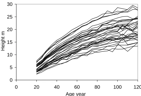
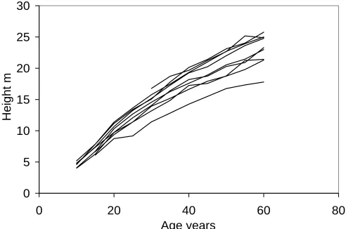
As the result of grouping, a total of 171 age-series of height, diameter, and volume were obtained. For il-lustration, empirical height series of pine, spruce, birch, and aspen stands are presented in Figures 1-4.
For evaluation of the model, data from the network of forest growth permanent sample plots in Estonia were used. The network of permanent sample plots was estab-lished in 1995–2004. By 2005 the first re-measurement data had been obtained from 380 sample plots. Of those, 93 sample plots were thinned during the period between measurements. The design and method of establishing and measuring permanent sample plots is described by A. Kiviste and M. Hordo (2002).
0 5 10 15 20 25 30
0 20 40 60 80 100 120
Age year
Height m
Figure 1: Height series of pine stands by forest site type.
0 5 10 15 20 25 30
0 20 40 60 80 100
Age year
Height m
Table 2: Maximum and minimum ages for stand selection, number of age-series and number of stands used for construction of series by dominant species and by stand origin (K – code of origin used in the model).
Species (Sp) Origin K Min. age Max. age No. series No. stands
Scots pine Naturally regenerated 0 20 120 34 151710
Scots pine Planted 1 20 120 28 54659
Norway spruce Naturally regenerated 0 20 100 25 55730
Norway spruce Planted 1 20 100 11 21180
Silver birch and downy birch Naturally regenerated 0 10 70 30 118080
Aspen Naturally regenerated 0 10 60 9 6557
Common alder Naturally regenerated 0 10 50 15 5170
Grey alder Naturally regenerated 0 10 50 9 9254
Common oak Naturally regenerated 0 20 120 3 822
Common oak Planted 1 20 120 3 205
Common ash Naturally regenerated 0 20 100 4 552
0 5 10 15 20 25 30
0 20 40 60
Age year
Height m
Figure 3: Height series of birch stands by forest site type.
0 5 10 15 20 25 30
0 20 40 60 80
Age years
Height m
Figure 4: Height series of aspen stands by forest site type.
3
Methods
In forest growth modeling, equations for predicting stand variables, for example height, are expressed usu-ally in the general form
H=f(A, HB,) (1)
where: H is height of the stand at age A; and HB is height of the stand at a base age B (site index).
In case we know stand height H1 at age A1, then for height prediction using equation (1), site index HB should be calculated first. Site index HBcan be obtained by solving the following equation:
H1=f(A1, HB). (2)
In most cases for solving equation (2), iteration methods are necessary. To reach a solution of necessary precision a few iteration steps are usually enough. However, iter-ation programming is quite a time-consuming and com-plicated task. In certain cases the iteration method may not converge. This disadvantage does not occur in the case of algebraic difference equations given in the general form
H2=g(A1, H1, A2), (3) where: H2 is the predicted stand height at any age A2; and H1 is the known stand height at given age A1.
A smart and interesting solution is the algebraic dif-ference equation by Cieszewski and Bella (1989) for the Hossfeld growth function. Hossfeld’s growth function is known in the form of
H = b0 1+ b1
Ab2
, (4)
where: H is stand height at the age A, and b0, b1, and b2 are the growth function parameters.
Supposing that the growth function passes a point of base age (B , HB), the function (4) can be presented as
H=HB·
1+ b1
Bb2
1+ b1
Ab2
, (5)
where: HB is stand height at a base age B (site index), and b1 and b2 are growth function parameters.
Cieszewski and Bella (1989) learned that parameters HB and b1of the growth function (5) are inversely pro-portional.
b1=
β
HB. (6)
Replacing the parameter b1 in the equation (5) with the relation (6) we get
H =HB+ β Bb2 1 + β/HB
Ab2
. (7)
Substituting the base age B and site index HB in equa-tion (7) with the variables A1and H1the following alge-braic difference equation is obtained (Cieszewski & Bella 1989).
H2=
H1+d+r 2+ 4·β
(H1−d+r)·Ab22
, (8)
where: d=Bβb2, and
r=
(H1−d) 2
+4·β·H1 Ab2
1
.
The difference equation (8) proved to be appropri-ate for modeling of dominant height growth of pine forests in Sweden on the basis of permanent sample plot data (Elfving & Kiviste 1997), for modeling of dominant height growth of birch forests in Sweden on the basis of tree increment core data (Eriksson et al 1997) and in other studies (Trincado et al 2003, Kasesalu & Kiviste 2001). These successful experiences encouraged us to use the same difference equation (8) for modeling the Estonian height, diameter, and volume series.
3.1 Estimating the model parameters. The al-gebraic difference equation (8) includes three arguments A1, H1 and A2 and three parameters B, β and b2. To
estimate the parameters of a difference equation, the stand growth data are usually presented as set of inter-vals{(A1, H1), (A2, H2)}. In previous studies the pa-rameter B (base age) was fixed by trial and error (Elfv-ing & Kiviste 1997, Eriksson et al 1997, Trincado et al 2003). For Estonian data we fixed the value 50 years for base age B. Parametersβ and b2 were estimated using the procedure of non–linear regression analysis on the interval data.
In site index models (Cieszewski & Bella 1989, Elfv-ing & Kiviste 1997, Eriksson et al 1997) parameters β and b2were considered as constants for each tree species for a certain geographical region. In that case model (8) presents a one-parameter set of growth curves upon the age/height plane. According to our previous studies (Kiviste, 1995) the growth curves depend on site index and on the site properties (thickness of organic layer). Thus the height, diameter and volume should be mod-elled as a two-parameter set of curves.
In this study we used a combined method. In the first modeling step of, a total of 171 age-series of height, di-ameter, and volume were approximated using the three-parameter Hossfeld function (4). Using the non-linear regression procedure NLIN of SAS software (SAS Insti-tute Inc. 1989) a set of parameters b0, b1, and b2were estimated for each height (H), diameter (D), and vol-ume (M) series. To distinguish the set of parameters we added a letter respectively, for example bH2 is the parameter b2 for mean height. For this model residual standard errors of 0.48 m, 0.66 cm, and 12.4 m3ha−1 were estimated in relation to the height, diameter and volume series, respectively.
The Analysis of Variance proved significant difference of the parameter bH2by tree species. The variability of the parameter bH2 by tree species is represented in the Figure 5. The different values of parameter b2 by tree species were observed on the box-plots of diameter and volume as well. Medians of parameter b2 for height, diameter and volume were estimated for each species (Table 3).
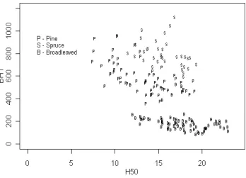
In the second modeling step, the inversely propor-tional relation of parameters bH1, bD1 and bM1 and variables H50, D50 and M50 were studied. The scatter-plot of the parameter bH1 against the site index H50 (Figure 6) shows large variation of the parameter bH1. Nevertheless, the inversely proportional relationship by species could be observed in the scatter-plots for height (Figure 6), diameter, and volume.
Figure 5: Box-plots of parameter bH2 by dominant species. bH2= parameter b2 for mean height.
layer is continuous, the other are discrete variables. For the covariance analysis, the procedure of general lin-ear methods (GLM) of the SAS software (SAS Institute Inc. 1989) was used. In the analysis, every series was weighted proportionally with the number of stands and inversely proportional with the residual variance calcu-lated at the first step of modeling. Only the significant variables (tree species, thickness of organic layer and origin of the stand, significance levelα= 0.05) were in-cluded in the model. The origin of the stand was set to 0 when the stand was cultivated (seeded or planted) and 1 when the stand was naturally regenerated. The following linear model was obtained:
β =C0+C1·ln(OHOR+ 1) +C2·K, (9) where: OHOR is the thickness of organic layer of soil cm; K is the dummy variable (Table 2); C0is a constant depending on tree species; and C1, C2 are other model constants.
4
Results
An algebraic difference equation was explored for pre-dicting stand height (H2), breast height diameter (D2) and volume (M2) at any age (A2) on the basis of the present state of stand description data (A1, H1, D1, M1). The algorithm is the following.
1. Determine the input values of the model:
- dominant tree species (pine, birch, spruce, aspen, grey alder, common alder, oak or ash);
- thickness of the organic layer of soil OHOR cm (Ta-ble 1);
- origin of the stand K (Table 2);
- stand age at a given moment A1 years;
- stand height (H1) m, diameter (D1) cm or volume (M1) m3ha−1 at a given moment;
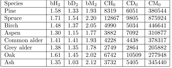
2. Find the constants bH2, bD2, bM2, CH0, CD0, and CM0 according to the dominant tree species (Table 3).
3. Calculate the coefficients ßH, ßD, and ßM of the equation (9) (LN is a function of the normal logarithm).
ßH = CH0 - 493·LN(OHOR + 1) + 1355·K; (10) ßD = CD0- 306·LN(OHOR + 1); (11)
ßM = CM0 - 54348·LN(OHOR + 1) + 56290·K. (12) 4. Calculate the variables dH, rH, dD, rD, dM and rM (SQRT is a function of the square root):
dH = ßH/50bH2 (13)
rH = SQRT((H1 - dH)2 + 4·ßH·H1/AbH1 2); (14) dD = ßD/50bD2 (15)
rD = SQRT((D1 - dD)2+ 4·ßD·D1/AbD1 2); (16)
dM = ßM/50bM2 (17)
rM = SQRT((M1 - dM)2 + 4·ßM·M1/AbM1 2). (18) 5. Calculate the predicted height (H2, m), diameter (D2, cm), and volume (M2, m3ha−1) at desired age A2. H2 = (H1 + dH+ rH)/(2 + 4·ßH·A−2bH2/(H1 - dH + rH)), (19)
D2 = (D1 + dD + rD)/(2 + 4·ßD·A−2bD2/(D1- dD + rD)), (20)
M2= (M1 + dM + rM)/(2 + 4·ßM·A−2bM2/(M1- dM + rM)). (21)
6. The algebraic difference model (10)–(21) can also be used for site index calculation. In this case the base age of site index (for example 100 years) should be as-signed to argument A2.
7. If we know the values of parameters H50, D50, and M50 for a certain site type then stand height, di-ameter, and volume can be predicted using the fol-lowing equations. Average values of parameters H50, D50, and M50 for most Estonian forest types are pre-sented in the worksheet ”Andmed” of MS Excel file (http://www.eau.ee/∼akiviste/kktab2.xls).
H = (H50+βH/50bH2)/(1+(βH/H50)·A−bH2), (22) D = (D50+βD/50bD2)/(1+(βD/D50)·A−bD2), (23) M = (M50+βM/50bM2)/(1+(βM/M50)·A−bM2). (24) The difference model (10)–(21) was fitted to the height, diameter, and volume series by finding the most suitable values of H50, D50and M50for each series. Pre-dictions for series were calculated from the state A1 = 50, H1 = H50, D1 = D50 and M1= M50. No signifi-cant bias between predictions and height, diameter, and volume series were found. The residual standard errors 0.57 m, 0.83 cm, and 17.0 m3ha−1 of the model were calculated in relation to the height, diameter and vol-ume series. These residual standard errors were slightly higher than those in the case of the Hossfeld function (4).
5
Model evaluation
The algebraic difference model (10)–(21) was evalu-ated on 287 permanent-sample plot data measured twice with an interval of 5 years in 1995–2004. The plots were located randomly in different parts of Estonia and the stands were not thinned between the two measurements. Also, plots with great mortality caused by natural dis-turbances were excluded from the analysis.
Data from the first measurement of plots (stand age, height, diameter, volume, thickness of organic layer of soil, stand origin, dominant species) were assigned to input variables of the model. Using the difference model, stand height, diameter, and volume were pre-dicted five years forward and compared with the plot re-measurement data.
re-Table 3: Parameter estimates for height, diameter and volume algebraic difference equations.
Species bH2 bD2 bM2 CH0 CD0 CM0
Pine 1.58 1.33 1.93 8319 6051 380544
Spruce 1.71 1.54 2.20 12867 9805 875924
Birch 1.48 1.37 2.05 4990 5034 446641
Aspen 1.30 1.15 1.77 3882 7092 310877
Common alder 1.41 1.41 1.93 4228 4438 378317 Grey alder 1.38 1.35 1.78 2749 2864 205882
Oak 1.61 1.45 2.02 6742 10509 277948
Ash 1.35 1.03 2.12 3732 5405 345440
sults of the second measurements and predicted values for stand height (EH), diameter (ED), and volume (EM) are presented.
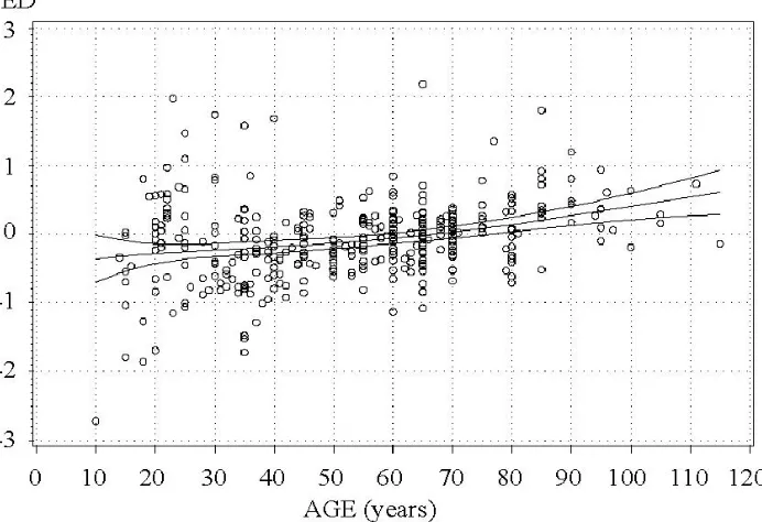
No overall bias of height and diameter growth predic-tions can be observed in Figures 7 and 8. The residual standard errors of five-year height and diameter growth predictions were 0.86 m and 0.58 cm respectively. How-ever, at young ages the model slightly overestimates and at mature ages underestimates the actual growth of height and diameter.
Such trends were not revealed when difference model predictions were compared with initial data (height, di-ameter, and volume series compiled from forest inven-tory data). However, a similar effect became evident when site indices of forest inventories in the 1950s and 1990s were compared (Kiviste, 1999). This trend could be explained by the hypothesis that forest growth condi-tions were improved and the stand growth was accelerat-ing in Estonia duraccelerat-ing the last decades (Nilson & Kiviste 1986).
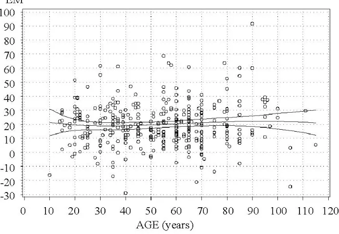
Figure 9 shows that volume growth predictions are on an average 20 m3ha−1 lower than their actual values by the permanent plot data. Apparently, this could be caused by the fact that thinned and seriously damaged stands were excluded from the comparison while most Estonian forest stand data (including thinned and dam-aged stands) was used for model building. The residual standard error of five-year volume growth predictions was 15 m3ha−1.
6
Discussion
In this study, a system of algebraic difference equa-tions for prediction of stand height, diameter, and vol-ume of Estonian forests have been explored. The model summarizes large amounts of forest inventory data which is its major advantage in comparison with previous mod-els and growth and yield tables used in Estonia. The model parameters cover a huge variety of forest site properties, which enables us to generalize forest growth
for different forest site types using a smart system of equations.
The structure of the model expressed in the form of algebraic difference equations is a convenient way of us-ing it and enables its easy employment in applications. The algebraic difference model (10)–(21) proved to be reliable and trouble-free and that is one reason why it is included into the Estonian state forest information system and into several software packages for forest in-ventory data processing.
The model (10)–(21) describes most reliably the growth of dominant forest types from the age of pole forests up to the age of matured forests. As a rule, model extrapolation beyond the range of initial data is not recommended. However, the basic function of the model is a classical Hossfeld growth function, which is one of the most suitable functions for forest growth mod-eling (Kiviste 1988, Kiviste et al 2002); thus we should obtain reasonable extrapolations even for young stands and over-matured stands.
Upon approximation of the height, diameter and vol-ume series, the number of stands was used as the weight of each observation. Therefore, the regularities of the most widely spread species like pine, spruce, and birch, and dominating site types likeMyrtillus, Rhodococcum, andAegopodium have been “imposed” on relatively un-common species and site types. Using the weight func-tion for modeling relafunc-tionships between parameters was necessary because series of rare forest types having a relatively low number of observations appeared too “er-ratic” to detect any regularities.
Figure 7: Errors in meters of the difference model for predicting five-year stand height growth, depending on stand age at first measurement. The trend curves show model bias and its 95% confidence limits. EH = H2actual – H2model
Figure 9: Errors in m3ha−1 of the difference model for predicting five-year volume growth, depending on stand age at first measurement. The trend curves show model bias and its 95% confidence limits. EM = M2actual – M2model.
from a well-designed set of permanent plots should be used.
The model is based on Estonian state forest inven-tory data collected in 1984–1993, grouped by forest type and age class. Those series express the relationship of how conditional average values of height, diameter, and volume are depending on stand age. These series can coincide with the real growth of the stands (assuming that the ocular estimates of forest surveyors are free of systematic errors) only when the growth conditions of the stands have been stable in time. Several studies, however, point at changing growth conditions, demon-strating a considerable increase in forest growth during recent decades (Nilson & Kiviste 1984, Eriksson & Jo-hansson 1993, Elfving & Tegnhammar 1996). In that case the model offered in this paper will actually give a bit smaller predict than realistic prognoses.
7
Conclusion
A method for construction of an algebraic difference model from forest inventory stand description data has been presented in this paper. Using this method, sys-tem of algebraic difference equations (10)–(21) have been explored for predicting stand height, diameter, and vol-ume growth on the basis of the present state of stand description data.
As initial data for this study, stand variables like total
age, average height, diameter, volume, stand origin, site type and stand composition by species from database files of all Estonian state forest districts have been used. Height, diameter and volume series on age were calcu-lated as averages of data groups by site type, by domi-nant species, by origin and by age classes of 5 years. A total of 171 data series has been created from 423,919 stand descriptions.
The Cieszewski, Bella (1989) algebraic difference equation (8) has been used for model construction. First, tree parameters of Hossfeld function (4) were es-timated for each of the height, diameter and volume se-ries, and later relationships between the parameters were studied.
Finally, an algebraic difference equation model (10)– (21) has been developed. Dominant tree species (Table 2), thickness of organic layer of soil (Table 1), stand origin (Table 2), height, diameter, and volume at given age were used as input variables of the model. Parameter estimates of the model are presented in Table 3 and in equations (10)–(12).
No significant bias between model predictions and ini-tial data (height, diameter, and volume series) were found. The residual standard errors 0.57 m, 0.83 cm, and 17.0 m3ha−1 of the model were calculated in rela-tion to the height, diameter and volume series.
of five years in 1995–2004. The residual standard errors of five-year height and diameter increment predictions were 0.86 m and 0.58 cm respectively. However, at young ages the model slightly overestimates and at mature ages underestimates the actual growth of height and diame-ter. Volume growth predictions were on an average 20 m3ha−1 lower than their actual values on the basis of the permanent plot data. This could be caused by the fact that thinned and seriously damaged stands were ex-cluded from the comparison while most Estonian forest stand data (including thinned and damaged stands) was used for model building. The residual standard error of five-year volume increment predictions was 15 m3ha−1. The structure of the model expressed in the form of al-gebraic difference equations is a convenient way of using it and enables its easy employment in applications. The model (10)–(21) proved to be reliable and trouble-free, which is one reason why it is included in the Estonian state forest information system and in several software packages for forest inventory data processing.
Acknowledgements
The study was supported by the Estonian Ministry Erratum:
9/6/09 of Education and Research (project SF0170014s08).
Thanks are due to the two anonymous reviewers for their help in improving the manuscript.
References
Cieszewski, C. J. and I. E. Bella. 1989. Polymorphic height and site index curves for lodgepole pine in Alberta. Can. J. For. Res. 19: 1151-1160.
Clutter, J. L., J. C. Fortson, L. V. Pienaar, G. H. Bris-ter and R. L. Bailey. 1983. Timber management: a quantitative approach. John Wiley & sons, New York, 333 p.
Elfving, B. and A. Kiviste. 1997. Construction of site index equations for Pinus sylvestris L. using perma-nent research plot data in Sweden. For. Eco. Man., 98(2): 125-134.
Elfving, B. and L. Tegnhammar. 1996. Trends of tree growth in Swedish forests 1953-1992. An analysis based on sample trees for the National Forest In-ventory. Scan. J. For. Res., 11: 26-37.
Eriksson, H., U. Johansson and A. Kiviste. 1997. A site-index model for pure and mixed stands of Betula pendula and Betula pubescens in Sweden. Scan. J. For. Res., 12(2): 149-154.
Eriksson, H. and U. Johansson. 1993. Yields of Norway spruce (Picea abies (L.) Karst.) in two consecutive
rotations in southwestern Sweden. Plant and Soil 154: 239-247.
Etverk, I., K. Karoles, E. L˜ohmus, T. Meikar, R. M¨anni, T. Nurk, J. Pikk, T. Randveer, ¨U. Tamm, U. Veibri and A. ¨Ord. 1995. Estonian forests and forestry. Tallinn. 128 p.
Kasesalu H. and A. Kiviste. 2001. The Kuril larch (Larix Gmelinii var. Japonica (Regel) Pilger) at J¨arvselja. Baltic Forestry 7(1): 59-66.
Kiviste, A. 1988. Forest growth functions. Tartu, 108 + 171 p. (in Russian)
Kiviste, A. 1995. Eesti riigimetsa puistute k˜orguse, diameetri ja tagavara s˜oltuvus puistu vanus-est ja kasvukohatingimustvanus-est 1984.-1993.a. met-sakorralduse takseerkirjelduste andmeil. Eesti P˜ollumajandus¨ulikooli teadust¨o¨ode kogumik. 181. Tartu, 132-148.
Kiviste, A. 1997. Eesti riigimetsa puistute k˜orguse, diameetri ja tagavara vanuseridade diferentsmudel 1984.-1993.a. metsakorralduse takseerkirjelduste andmeil = Difference equations of stand height, diameter and volume depending on stand age and site factors for Estonian state forests. Eesti P˜ollumajandus¨ulikooli teadust¨o¨ode kogumik. 189. Tartu, 63-75.
Kiviste, A. 1999. Site index change in the 1950s–1990s according to Estonian forest inventory data. Causes and consequences of accelerating tree growth in Eu-rope. EFI Proceedings 27: 87–100.
Kiviste, A., J. G. Alvarez Gonzalez, A. Rojo Alboreca and A. D. Ruiz Gonzalez. 2002. Funciones de crec-imiento de aplicacion en el ambito forestal. Madrid, 190 p.
Kiviste, A. and M. Hordo. 2002. Eesti metsa kasvuk¨aigu p¨usiproovit¨ukkide v˜orgustik = Network of permanent forest growth plots in Estonia. Met-sanduslikud uurimused 37. Tartu, 43–58.
L˜ohmus, E. 1984. Eesti metsakasvukohat¨u¨ubid = Es-tonian forest site types. Tallinn, 88 p.
Nilson, A. and A. Kiviste. 1986. Reflection of envi-ronmental changes in models of forest growth com-posed using different methods. Monitoring of forest ecosystems. Abstracts of scientific conference. Kau-nas, 05-06.06.1986. Kaunas-Academy, 336-337. (In Russian).
Rayner, M. E. 1991. Site index and dominant height growth curves for regrowth karry (Eucalyptus di-versicolor F. Muell.) in south-western Australia. For. Eco. Man., 44: 261-283.
Rennolls, K. 1993. Forest height growth modelling. Growth and yield estimation from successive forest
inventories. Proceedings from the IUFRO confer-ence, held in Copenhagen, 14-17 June. 231-238.
SAS Institute Inc. 1989. SAS/STATr User’s Quide, Version 6, Fourth Edition, Vol. 2, Cary, NC: SAS Institute Inc., 846 pp.
Trincado, G., A. Kiviste and K. von Gadow. 2003. Preliminary site index models for native Roble (Nothofagus obliqua) and Rauli (N. alpina) in Chile. New Zealand Journal of Forest Science 32(3): 322-333.